


Asset owners responsible for the management and maintenance of bridges value the collection of data that can be processed into useful information to inform decisions about future management of structures. Installing, powering and receiving data from sensors is not always convenient or possible, but satellite monitoring may provide the ability to measure bridge movements and thus provide an indication of potential problems for asset owners to take action on. This study presents the results of satellite monitoring of the Hammersmith flyover, London, UK, using the interferometric synthetic-aperture radar (InSAR) technique. Sentinel-1 (free) and Cosmo-SkyMed (commercial) satellite radar data were processed to provide millimetre-scale measurements of the flyover and surrounding region and validated with in situ sensor measurements. A method was developed for selecting and comparing InSAR measurements with in situ displacement and temperature measurements, making use of bridge geometrical and structural modelling information. The results compare in situ sensor measurements with remote InSAR measurements and show the suitability of such measurements in measuring thermal expansion for some (but not all) bridge assets. The proposed techniques, illustrated with the case study of the Hammersmith flyover, will enable asset owners to collect regular measurements of bridge movements to complement and add value to current inspection methods and potentially give early warning to defective bridge bearings.
Notation
- F(ω)
Fourier transform
- Î
horizontal unit vector in the satellite line-of-sight (LOS) direction
- k
thermal dilation parameter
- N
data size
slant range difference in the LOS direction
- û
unit vector along the bridge
- vi
velocity of pixel i
- α
ground heading angle for the selected pixel
- ΔD
measured linear variable differential transformer deformation difference
- ΔTj
temporal baseline of the interferogram j
- ΔTemp
recorded temperature difference
unwrapped phase of pixel i in the interferogram j
- θ
incidence angle (look direction angle to the vertical axis)
- λ
transmitted radar wavelength
- σ
standard deviation
- Φ
angle of the bridge with the north direction in the horizontal plane
- φ
phase change between transmitted and received signals
- φres
residual phase
- ω
frequency of signal
1 Introduction
The management of transport infrastructure is critical for public safety and local economies. The monitoring and maintenance of ageing and deteriorating assets is a key challenge for asset owners. A study by the RAC Foundation and the UK National Bridges Group of the Association of Directors of Environment, Economics, Planning and Transportation in 2020 highlights that 4.3% of all local authority bridges in the UK are classified as ‘substandard’, with a £5.55 billion maintenance backlog for local authority bridges (RAC Foundation, 2020). In the USA, 9.1% of the nation’s bridges were found structurally deficient in 2016, with a US$123 billion maintenance backlog (ASCE, 2017).
Bridge owners require a management cycle, which involves inspecting, maintaining and, where appropriate, rehabilitating deteriorating bridge stock (Bennetts et al., 2016). This management cycle usually relies in the first instance on a system of periodic visual inspections at an interval in the range of several years. Visual inspections are a relatively cost effective and simple approach to collecting information about the condition of a structure (McRobbie et al., 2015). The subjective nature of human judgement is useful in identifying non-standard behaviours and applying a case-specific approach, but previous studies (Moore et al., 2001) highlight that they do not necessarily provide reliable results. It is also difficult for the human eye to spot changes in the expansion and contraction of bridges facilitated by bearings, expansion joints and other articulation. A balance also needs to be struck between having regular asset monitoring and the cost of doing so, both financially and with regard to the disruption caused to the network (e.g. by bridge closure). Consequently, inspections are typically carried out every few years. It has been suggested that structural health monitoring (SHM), using sensing technologies to take more frequent readings, could provide more objective and repeatable data to supplement visual inspections and manage risk (Bennetts et al., 2016; McRobbie et al., 2015).
Earth observation data from satellites are becoming more accessible, and with improving spatial and temporal resolution. These data can provide a means of remote monitoring that covers large geographical regions. They can also provide insights into infrastructure assets that are difficult to access or monitor regularly with conventional approaches. Within the asset-management context outlined, satellite monitoring provides the opportunity to collect information related to an asset remotely every few days. Thus, there are opportunities in being able to monitor for signs of unusual behaviour that develop in the periods between inspections or are not picked up visually. Remote satellite monitoring offers a further advantage over traditional in situ sensor monitoring in that it does not require an electrical connection or a power source at the site or closure and physical access to the bridge. Interferometric synthetic-aperture radar (InSAR) is a specific Earth observation technique that makes use of the differences between radar images to measure millimetre-scale movements of specific points within the image and provides an opportunity to enhance current bridge-monitoring practices.
The opportunities that bridge engineers could consider for InSAR monitoring include the ability to collect regular readings. For example, free Sentinel synthetic-aperture radar (SAR) imagery is available every 6 days in European locations and every 6 or 12 days in most of the rest of the globe, courtesy of the European Space Agency (ESA). Remote satellite monitoring also avoids some of the problems encountered on-site, such as finding a suitable electricity source for sensors, finding that sensors are down for some reason or installing equipment on remote or hard-to-access sites. Archives of previously acquired images mean that measurements of historical movements can also be analysed in a study of a structural asset or ground area, to understand past events or establish baselines of ground movements. The large coverage of the image footprint provides the opportunity to investigate wide-area effects (e.g. settlement due to phenomena such as mining or dewatering). When combining InSAR measurements with other sensor and in situ data, the benefits of both forms of measurement are brought together, and their combination can provide new and useful insights for specific contexts and projects.
This study examines the use of InSAR in the practical application of bridge monitoring, with the purpose of understanding how remote monitoring could be used to spot unusual movements in bridge assets, and provides civil engineers with an understanding of how to deploy such technologies appropriately. The next sections of this paper are structured as follows: Section 2 provides a basic outline of the theory behind InSAR technologies and their application in the civil engineering and bridge sectors. Section 3 introduces the Hammersmith flyover as the case study for this work. Section 4 explains the experimental set-up for both in situ sensor monitoring and InSAR satellite monitoring. Sections 5 and 6 present the results and outline some of the challenges associated with interpreting InSAR data in the context of bridges within two urban environments. Section 6 also describes a methodology by which the results could be more easily interpreted. In Section 7, a comparison of InSAR data and in situ monitoring data is undertaken, and the authors suggest a means of using InSAR analysis to identify defects in bridge articulation. Finally, Section 9 presents a discussion on the suitability of InSAR for bridge monitoring before concluding the paper in Section 10.
2 InSAR theory
SAR imaging has been used as a remote sensing method for over 30 years, for observing various phenomena such as earthquakes (Massonnet et al., 1993), observing volcanoes (Massonnet et al., 1995), flood mapping (Oberstadler et al., 1997) and sea and ice classification (Dierking, 2013). It is an active remote sensing system that acquires data by sending and receiving microwaves (in the invisible part of the electromagnetic spectrum) with wavelengths in the millimetre to metre range. SAR satellites operate using specific wavelengths in the electromagnetic spectrum, with the L-band, C-band and X-band being the predominant wavelengths available in both various commercial satellites and satellites generating openly available data. Unlike optical imaging systems (which use light waves), SAR is able to penetrate through clouds and precipitation and can also be used both day and night irrespective of the sun illumination of the ground. Thus, SAR provides a technology that can provide high-resolution, all-weather imaging with global coverage.
2.1 SAR imaging
Satellites with the objective of SAR data collection are usually designed to follow a near-polar orbit (i.e. they travel in a north–south direction from pole to pole) around the Earth. The satellites travel northwards on one side of the Earth (the ascending pass) and then towards the south pole on the second half of their orbit (the descending pass). As they pass over the Earth, they acquire images by emitting and receiving radar pulses with a side-looking perspective (Figure 1). This imaging geometry means that SAR satellites are more sensitive to capturing deformation changes in a vertical direction and an east–west direction, and only part of any deformation occurring north–south direction is captured. This point is particularly relevant for bridge monitoring, with results being affected by bridge orientation (Selvakumaran et al., 2020).
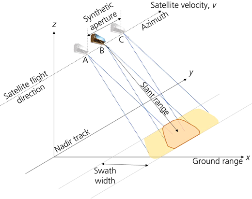
The pixels in a SAR image are associated with an area on the Earth’s surface (the size of the resolution cell varies with each satellite) but taken in SAR imaging coordinates, with axes in the azimuth (direction of the satellite flight path) and the range (perpendicular to the flight path). Each pixel contains an associated phase value and an amplitude value connected to a reflected SAR signal.
A geocoding process is required to associate each pixel in the SAR image with a position on the ground. Before interpreting InSAR results, it is important for bridge engineers to appreciate that there are SAR imaging effects and that the SAR images do not necessarily map directly to classical geographic references and optical images, as they are used to seeing. For example, SAR images typically appear geometrically distorted. In a radar image, the three-dimensional (3D) objects of the scene are mapped to a two-dimensional (2D) image in the slant range and azimuth. This results in effects such as foreshortening, layover and radar shadows (explained in further detail below). This topographic distortion can sometimes be removed using a digital elevation model (DEM), but buildings are not always included in DEMs of lower resolution.
2.2 Multi-temporal InSAR
The satellite generates the outgoing SAR signal (with a known phase), which can then be compared to the phase of the return signal, which is dependent on the precise distance to the ground in the line of sight (LOS) of the satellite (Figure 2). This distance is a phase measurement represented as Nλ + φ = [0–2π] radians, where λ is the transmitted wavelength; φ is a phase change between transmitted and received signals; and N is large, but unknown. When the complex signal information of one image is multiplied by the complex conjugate signal of another image, an ‘interferogram’ is formed. This results in the common backscatter phase in pixel being cancelled while leaving a phase term proportional to the differential path delay. Differential InSAR makes use of differential interferograms (two interferograms), to compute the deformation of the observed area (Figure 2).
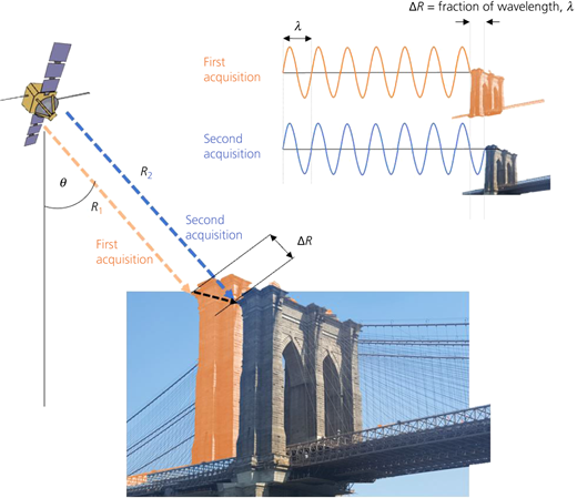
Multi-temporal InSAR techniques involve processing multiple differential interferograms from a stack of SAR acquisitions over the same area to allow for the correction of phase contributions such as atmospheric effects and noise and therefore reduce the errors associated with the deformation estimates. The end result is a time series measuring change in deformation in the LOS of the satellite over time, relative to the first acquisition in the stack.
There are several established multi-temporal InSAR approaches to extract this LOS motion using SAR images. Objects are monitored using the coherent processing of backscattered signals from multiple distributed targets within a SAR resolution cell. Any objects causing scattering of a SAR signal are called scatterers. The choice of method is based on the scattering mechanism of the target being studied. Objects whose response to radar is a strong reflection that is constant over time can be picked up using the persistent scatterer interferometry (PSI) approach (e.g. Ferretti et al., 2000, 2001). The PSI technique relies on analysing scatterers that remain coherent over a sequence of acquisitions. In practice, this is used for rocks or urban environments that provide suitable dominant reflectors. It is also important to note that these are single scatterers inside a resolution cell, which allows large perpendicular baselines to be used. This is the distance between the locations of the satellite at each acquisition. For multiple scatterers, the satellite is required to be in approximately the same position in space each time that an acquisition is taken. The small baselines subset (SBAS) approach (Berardino et al., 2002) inverts a network of interferograms with small temporal and perpendicular baselines. This method is used for distributed targets (but also works for persistent scatterers). This method involves inverting a network of interferograms with small temporal and perpendicular baselines. It is suited to rural areas where there are fewer strong and dominant objects acting as natural reflectors. There are several other variations of these algorithms which build on these two methods, and a review and comparison of different methods in the literature is presented by Crosetto et al. (2015) and Hooper et al. (2012). For all of these methods, the images in the stack must be acquired over the same area, using the same imaging geometry. This includes being in the same flight direction, polarisation, look direction angle to the vertical axis (known as incidence angle) and mode. Typically, this is found by using the images from one satellite or a constellation from the same provider.
Within the context of bridge monitoring, the type of SAR imaging and InSAR processing techniques employed affect the type of deformation that can be monitored. The maximum movement over time (velocity) that can be detected would depend on factors such as the radar wavelength, the spatial density of the scatterers and the temporal sampling of the acquisitions (as defined by the revisit time of the SAR satellite). Considering the wavelength and revisit time of the TerraSar-X and Sentinel-1 satellites as an example, the maximum differential deformation rates measurable are 25.7 and 42.6 cm/year, respectively (Crosetto et al., 2015). These values are theoretical and in practice also depend on the noise level of the data and the specific methodologies used to resolve phase ambiguities.
2.3 Applications of InSAR
Satellite-based InSAR techniques have already been deployed in the past few decades to detect small displacements of the Earth’s surface over a wide range of applications. Applications useful for civil engineers include the monitoring of tunnel deformation (Giardina et al., 2019; Perissin et al., 2012), landslides (Schlögel et al., 2015), road and railway networks (Chang et al., 2018) and subsidence (Peduto et al., 2017). Looking at the study of bridges specifically, there have been a number of exploratory studies and growing interest in applying InSAR to bridge monitoring. These include studies on specific large bridge assets (Cusson et al., 2018; Hoppe et al., 2019), including comparison between observed displacements and model estimates (Cusson et al., 2021). The technology has also been used to study historic bridge failures, using archive satellite data to investigate whether any signs or precursors to failure could have been picked up (Milillo et al., 2019; Selvakumaran et al., 2018; Sousa and Bastos, 2013). Accounting for thermal dilation in bridges is a significant consideration, and studies on this topic to date include those by Lazecky et al. (2017), who monitored several highway bridges to isolate the seasonal component of the deformation signal, and Zhao et al. (2017), who monitored the linear deformation at key points along a steel arch structure, correlating these movements with the thermal response. A major limitation of InSAR measurements is the one-dimensional (1D) LOS measurement, and this consideration of 3D deformation of bridges with respect to InSAR measurements (and the ability to combine different viewing geometries to overcome this limitation in specific cases) has also been considered in a few studies (Huang et al., 2018; Qin et al., 2018; Selvakumaran et al., 2020).
2.4 Measurement accuracy and uncertainty
To use InSAR for bridge monitoring, it is important to consider the scale of measurement accuracy that InSAR can provide. The measurement accuracy is generally accepted to be sub-centimetre, and there are many studies in the literature that prove this using field data. For example, Marinkovic et al. (2008) conducted an experiment comparing corner reflectors (objects that reflect most incident energy back towards the satellite, to provide a known reflection point within a SAR image) with levelling observations, reporting vertical differences of 2.8 mm for data from the Envisat satellite and 1.6 mm for data from the ERS-2 satellite.
It has also been proven that the technology can measure relative movements to sub-millimetre accuracy (Ferretti et al., 2007a), but it should be noted that this result shows that such accuracy is possible within a specific and controlled case but may not be achieved in day-to-day use monitoring structures in practice. Quin and Loreaux (2013) deployed a network of specially developed reflectors, which were moved using micrometric vernier controls, and reported that the relative displacements between the reflectors had a standard deviation of 0.48 mm along the LOS direction using TerraSar-X satellite data. Note that in this example, this is in the LOS of the satellite and further measurement uncertainty is introduced in taking a specific component (e.g. vertical component) of this measurement.
The measurements in these studies were made by using the difference in the phase value between corresponding pixels in each SAR image. InSAR time series processing involves a complex estimation process in which the selection of different processing parameters and processing algorithms can result in different results and estimates of uncertainty even when studying the same stack of data. There are several large-scale studies comparing InSAR deformation time series readings (or deformation velocities calculated from these results) with independent estimations of the same quantities acquired by other measurement techniques (e.g. levelling). For example, Raucoules et al. (2009) showed a standard deviation of measurements of between 0.6 and 1.9 mm/year. Validation of these velocity rates against rates measured on the ground showed a variation of between 5 and 7 mm/year, with some discussion on the measurement uncertainty. This included considering the precision of the automated electronic levels used for on-site monitoring being up to 1.5 mm and noting that the points measured by the satellite were not always exactly the same as the levelling points and comparing measurements included some interpolation. These considerations could affect the final measurement validation results. Crosetto et al. (2008) and Adam et al. (2009) showed standard deviations of the deformation velocity of between 0.4 and 0.5 mm/year. If looking at these results for the time series as individual measurement readings (rather than a best fit of points to calculate velocity), the standard deviation was found to be between 1.1 and 4.0 mm. Validation of these velocity rates against rates measured on the ground in this study found the standard deviation to be between 1.0 and 1.8 mm/year (and for time series measurements, it was between 4.2 and 6.1 mm).
Sadeghi et al. (2021) compared different InSAR time series processing methods to evaluate differences in output between these methods as applied to the same SAR Sentinel-1 data sets. Each of the InSAR processing methods was able to detect similar deformation signals in a defined area, and all of the methods tested provided a good density of selected scatterers in urban areas. However, the deformation velocities (rate of deformation over time, millimetres per year) calculated for each scatterer and the time series products (plot of movement in the LOS of the satellite against time) were not completely identical. The average of the standard deviations of velocity differences for all InSAR inter-comparison pairs was 1.1 mm/year, with all comparisons being better than a 2 mm/year variation. The average of the standard deviation of deformations measured in the time series ranged between 1 and 2 mm. The study also showed that for scatterer pixels in a specific area where deformation was occurring processed by different methods, over half of the pixels showed a consistent deformation pattern across the different processed sets. Methodology choice in processing and criteria used for selecting pixels produced variations in point density and coverage. In comparing the results produced by all of the studied methods, the density of pixels varied from approximately 200 pixels/km2 found in a densely vegetated area to approximately 5600 pixels/km2 found in an urban area. The coverage – that is, the percentage of 100 × 100 m grid pixels containing at least one measurement – had a best coverage of 42% in rural areas and 100% in urban areas.
3 Study site
The Hammersmith flyover in London, UK, was constructed in the 1960s as a strategic road asset carrying four lanes of traffic in and out of London from the west (Figure 3). It is a 622 m long post-tensioned prestressed concrete segmental bridge. It was considered to be an innovative structure in its time and is the first major segmental precast post-tensioned highway structure in the UK. It is made up of 16 spans (typically 42 m long) forming a single, central spine beam with transverse cantilevers supporting the roadway. The two abutments (A and Q) are at each end of 15 piers (labelled B to P) as shown in Figure 4. The bridge is articulated by roller bearings at the base of each of the 15 piers and one expansion joint located in one of the centre spans separating the superstructure into two structurally independent sections. Longitudinal restraint is provided at the abutments at either end of the bridge.

Photograph of the Hammersmith flyover at street level below the bridge. Photograph reproduced with the kind permission of Ramboll UK
Photograph of the Hammersmith flyover at street level below the bridge. Photograph reproduced with the kind permission of Ramboll UK
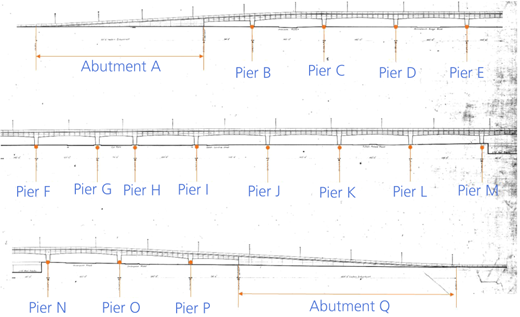
General arrangement drawing of the Hammersmith flyover with abutments and piers labelled. The distance between piers is 140 feet (42.7 m) with the exception of AB and PQ (94 feet 6 inches or 28.8 m), GH (74 feet or 22.6 m), HI (120 feet or 36.6 m) LM (139 feet or 42.4 m) and MN (141 feet or 43.0 m)
General arrangement drawing of the Hammersmith flyover with abutments and piers labelled. The distance between piers is 140 feet (42.7 m) with the exception of AB and PQ (94 feet 6 inches or 28.8 m), GH (74 feet or 22.6 m), HI (120 feet or 36.6 m) LM (139 feet or 42.4 m) and MN (141 feet or 43.0 m)
3.1 Background to monitoring work
The bridge experienced a number of problems leading to its closure during the Christmas period in 2011, causing severe disruption to traffic and the local economy. The reason for closure was primarily due to severe corrosion of the prestressing tendons within the flyover, accelerated by increased use of de-icing salts on the road. The flyover was not originally designed to be subjected to de-icing salt, as designers provided electric deck heating. However, this system became defective and stopped working at some point in the decades prior to the closure of the bridge in 2011.
Also, visual inspection of the bridge revealed concerns regarding bridge bearing performance at multiple locations. Bearings allow bridges to move under imposed loading, and the seizing or restricted movement of bearings can lead to significant problems due to restraint against expansion. This restraint could cause additional bending moments in the deck and induce stresses that the bridge was not designed to withstand. For this reason, it is important to inspect bridge bearings regularly and also ensure that they are able to move. If they are not able to move, further analysis should be undertaken to understand the level of damage imposed and identify whether replacement is needed.
4 Deployed monitoring systems
4.1 Traditional monitoring systems
From 2010 to present, the bridge has been fitted with a number of different monitoring systems. These include a vast range of sensors, including approximately 300 acoustic emission sensors to detect wire breaks in the prestressing tendons, temperature sensors, inclinometers and strain gauges on the piers and displacement transducers and automated total stations to detect and measure pier displacement. The bridge was also used to test a novel wireless sensor SHM system to showcase the application of wireless sensor networks in parallel with wired monitoring solutions. The result is a patchwork of different data sources at various time periods between 2010 and 2018. More specific details regarding different aspects of these deployments on the Hammersmith flyover are described in the publication by Webb et al. (2014).
For the purpose of this study, only those deployments providing information on thermal expansion of the bridge were considered. Systems such as acoustic emission monitoring to detect wire breakages within the prestressing tendons were not taken into account, as such defects cannot be picked up through the monitoring of displacements of the deck. Data from the following existing sensor systems were used:
temperature sensors embedded in the top, bottom and web of the deck at four midspan locations of the bridge – spans BC, FG, KL and OP
displacement transducers (linear variable differential transformers or LVDTs) used for measuring linear displacement at bearing locations at the base of each of piers B to P (Figure 5).
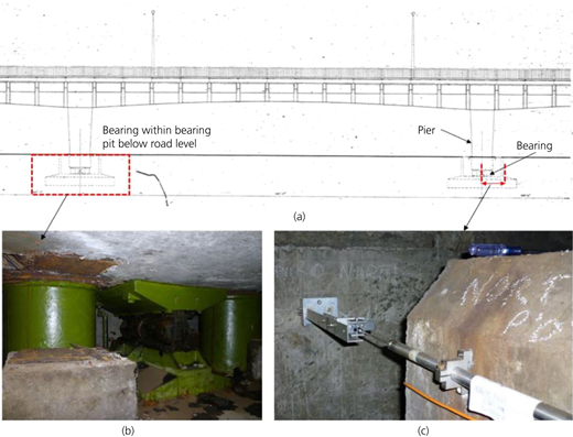
LVDT installation for bearing movement measurement. Bridge drawing (a) illustrating location of bearings and bridge sections shown in photographs. Photographs showing (b) the bearing within the bearing pit and (c) LVDT installation between the wall of the bearing pit and the base of the pier. Photographs taken by and included with permission of Graham Webb
LVDT installation for bearing movement measurement. Bridge drawing (a) illustrating location of bearings and bridge sections shown in photographs. Photographs showing (b) the bearing within the bearing pit and (c) LVDT installation between the wall of the bearing pit and the base of the pier. Photographs taken by and included with permission of Graham Webb
During the period of this study, one of the existing SHM schemes was removed by a contractor and later replaced with another, intended for longer-term installation and monitoring of the bridge. The earlier scheme provided data for the period from August 2010 to August 2015 and the later installation uploaded data measurements from the bridge onto an online portal from September 2015 to November 2018.
4.2 InSAR satellite monitoring systems
There are currently a number of operational radar satellites that are able to image in different spatial resolutions (different pixel sizes depending on the mode of image acquisition and band of radar). Civilian SAR satellites have been available as data sources since the early 1990s, and it is worth noting the opportunity to use data archives to look back historically at assets. The Sentinel-1 constellation was launched as two satellites (one in 2014 and a second in 2016). Together they provide images over the same area every 6 days. This satellite constellation provides a frequent repeat cycle, and the ESA provides this SAR imagery free of charge. However, the spatial resolution is approximately 20 m by 4 m. This affects the point density of scatterers on a single bridge or infrastructure asset. There are a number of SAR satellites that provide a finer pixel resolution. Bovenga et al. (2018) summarise many of the current SAR satellite missions and some key details related to each constellation.
Two forms of SAR data were used for this study. Sentinel-1 data provided by ESA as outlined above and data from the Cosmo-SkyMed constellation operated by the Italian Space Agency (ASI) were used. The Cosmo-SkyMed images were acquired using X-band radar waves (31 mm wavelength) in ‘Stripmap’ mode for acquisition (3 m by 3 m pixel sizes in the azimuth and ground range directions).
Sentinel data collected from the ‘ascending’ pass – that is, on a satellite flight path south to north, 132 tracks between November 2015 and October 2017 – were used for a general comparison with Cosmo-SkyMed data and for evaluating the agreement between the InSAR measurement results and the ground-based measurements for the Hammersmith flyover. Sentinel data collected from the ‘descending’ pass were also processed to compare with the ascending data. These Sentinel data were processed using the open-source software package Stanford Method for Persistent Scatterer (StaMPS) (Hooper et al., 2007). Shuttle Radar Topography Mission (SRTM) data with a resolution of 3″ (90 m) was used as a DEM during the interferometric processing, to determine preliminary information about the height of the persistent scatterers.
Two stacks of Cosmo-SkyMed X-band SAR Stripmap mode data were also used in this study. The first data set of 40 Cosmo-SkyMed SAR acquisitions taken over the London region for the period from 2011 to 2015 were processed by e-Geos and provided by Telespazio Vega. The authors processed a second data set of 34 Cosmo-SkyMed SAR acquisitions collected from 2015 to 2018 using PSI methods implemented by the SARscape software package. For this second data set, SRTM data with a resolution of 3″ (90 m) was again used as DEM during the interferometric processing.
Thus, for this work on the Hammersmith flyover, three sets of PSI results were produced: one set of Sentinel-1 data and two sets of Cosmo-SkyMed data. The Cosmo-SkyMed sets comprised one for the 2011–2015 period and a second for the 2015–2018 period (with persistent scatterers different from those in the first Cosmo-SkyMed data set). The images in both stacks were acquired in the descending direction with an incidence angle varying between 25.1 and 27.9° across the image.
5 Results
Figure 6 shows a typical output from PSI processing comparing Sentinel and Cosmo-SkyMed Stripmap data. These are displayed in the open-source geographic information system (GIS) software package QGIS, where persistent scatterers are marked as dots (coloured by velocity calculated as a linear fit of displacement over time). Each of these data points contains a history of LOS movement over time, as well as characteristics describing the behaviour of the output products from the PSI processing (e.g. coherence value and linear average velocity in millimetres/year). There are three important considerations relevant to end users interpreting these initial results. Firstly, the persistent scatterer ‘dots’ represent the point target response within a particular pixel or combination of pixels attributed to an object. Secondly, the radar reflections collected back to the SAR sensor may not come from a single, direct reflection but instead may have been reflected multiple times or may appear distorted on the SAR image due to various imaging effects (Figure 7). The third point to note is that the images are acquired in SAR coordinate systems (range–azimuth). Part of InSAR processing includes a geocoding stage, where the SAR coordinates are mapped onto geographical coordinates. In this case, the results were mapped onto the World Geodetic System 84 coordinate system, to display the Cartesian coordinates of the persistent scatterers on a map (or optical image), which can be physically interpreted. These three considerations result in the physical interpretation of these scatterers being less than straightforward.
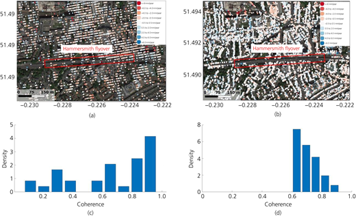
PS points derived from (a) Sentinel-1 C-band SAR data and (b) Cosmo-SkyMed X-band SAR data on the Hammersmith flyover and surrounding area overlaid onto OpenStreetMap base imagery. The graph in (c) shows the normalised histogram of coherence for the InSAR points selected by the Sentinel-1 data inside the red outlined rectangle in (a), and the graph in (d) shows the normalised histogram of coherence for the InSAR points selected by the Cosmo-SkyMed data inside the red outlined rectangle in (b). Note that the values below a specified coherence threshold were discarded for (d). Using these would have increased the density of points but would not be as reliable as those above the threshold
PS points derived from (a) Sentinel-1 C-band SAR data and (b) Cosmo-SkyMed X-band SAR data on the Hammersmith flyover and surrounding area overlaid onto OpenStreetMap base imagery. The graph in (c) shows the normalised histogram of coherence for the InSAR points selected by the Sentinel-1 data inside the red outlined rectangle in (a), and the graph in (d) shows the normalised histogram of coherence for the InSAR points selected by the Cosmo-SkyMed data inside the red outlined rectangle in (b). Note that the values below a specified coherence threshold were discarded for (d). Using these would have increased the density of points but would not be as reliable as those above the threshold
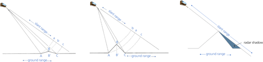
SAR sideways-looking imaging showing foreshortening (left), layover (middle) and radar shadow (right) effects. Points A, B and C are points on the ground that are being imaged. These points appear as a, b and c, respectively, on the SAR image
SAR sideways-looking imaging showing foreshortening (left), layover (middle) and radar shadow (right) effects. Points A, B and C are points on the ground that are being imaged. These points appear as a, b and c, respectively, on the SAR image
The density of selected persistent scatterer (PS) points for the Cosmo-SkyMed products was approximately 3 × 10⁴/km2 around the Hammersmith flyover. This is much higher than the output for the Sentinel-1 data, which was 3 × 10³/km2 around the Hammersmith flyover. This is attributed to the higher spatial resolution of Cosmo-SkyMed with respect to the Sentinel-1 data, but it should be noted that the measurement of deformation quality is similar for the two products. A higher spatial resolution does not necessarily mean better measurement quality.
The authors then interpreted InSAR processing results and extracted the relevant persistent scatterers of interest for this study (i.e. those that represented the movement of the flyover). The PSI processing of the image stack results includes the calculation of the coherence of the reflections being processed. Coherence (or correlation) is an estimate of phase noise, usually estimated by the correlation of phase with neighbouring pixels. Persistent scatterers below a specified coherence threshold of 0.65 were discarded. The location and time series for the remaining persistent scatterers can then be studied.
There are a number of methods and tools to aid in interpretation of InSAR data. A simple means is for a user to use the output overlaid onto a map or image to attribute more ‘obvious’ persistent scatterers that follow a line corresponding man-made objects (e.g. facades of buildings or metal parapets or edge beams of bridges). This does not deal with the challenges associated with particular imaging effects caused by SAR imaging geometry in urban areas. It is also possible to simulate the reflections through ray tracing (Auer et al., 2010) with software packages specifically developed to simulate SAR reflections against urban objects to interpret reflections (Auer et al., 2016).
6 Supporting interpretation of InSAR results
To understand some of the InSAR processed PS location results, the following section reviews some of the SAR imaging effects that would affect bridges in urban scenarios, such as the Hammersmith flyover, which is surrounded by buildings and other structures. When looking at the persistent scatterers overlaid onto map imagery (Figure 6), it can be seen that there are a number of regions on the bridge missing persistent scatterer points. The bridge has a consistent form and structure, which would suggest that each section should be equally suitable for PSI application. However, the viewing geometry of a SAR image results in certain geometric distortions on the resultant imagery (Figure 7). The side-view imaging in the slant-range direction causes effects such as foreshortening, layover and radar shadows. This can be particularly problematic in urban settings with high-rise structures.
6.1 Digital modelling
Overlay of PSI results onto 3D representations of buildings and other assets to aid interpretation has become common practice in recent years. Within traditional civil engineering and asset-management practice, the management and exchange of data related to a built asset is addressed by the information technology approach known as building information modelling (BIM). This often includes the production of geometrical models of assets, which can also support the interpretation of PSI results. In this study, the authors use a 3D model produced Ramboll UK, as part of a BIM model for Transport for London, and an online software package called GeoBIM (by Group BC), to import the geometric model of the Hammersmith flyover into a GIS space. Ordnance Survey mapping and building height data were then used to input 3D representations of the buildings around the bridge. Finally, the persistent scatterers were imported and overlaid onto the 3D representation of the Hammersmith area.
The persistent scatterers identified in the PSI processing come with an estimate of the location in (x, y, z) Cartesian coordinates. The height and deformation estimates of all PS points are made relative to a reference, or a ground control point (GCP), which can be selected based on a PS at a point known to be stable or at a point where the displacement is known (and can be input into the processing). If a known GCP is not input, the PSI process can assume a height value, which is extracted from the external DEM supplied during processing, for this GCP. If the reference point is not stable in time or its true absolute height value is not equal to the corresponding DEM height, the resulting height and deformation estimates will be biased by these effects.
In terms of 3D positioning, the absolute position accuracy of SAR scatterers has been demonstrated to be on the centimetre scale for 2D radar coordinate positional accuracy (Dheenathayalan et al., 2016) and in the tens of centimetres in 3D positioning error (Dheenathayalan et al., 2018), but with a potential of being as small as 2.6 cm for X-band data (Eineder et al., 2011). Combining this with the earlier note on ambiguity on the (x, y) plane highlights the uncertainty in interpretation and 3D positioning while still achieving millimetre-scale differential measurement between images.
Overlaying the InSAR persistent scatterer locations on the Hammersmith flyover 3D model and surrounding building models derived from Ordnance Survey data (Figure 8) provides a means to interpret which persistent scatterers are more likely to come from the bridge. In this particular example, it would be more useful to understand specifically which particular pier and side of bridge the persistent scatterers come from, in order to understand which part of the bridge the measured motion represents. To this aim, the authors developed a process to narrow down the selected points.
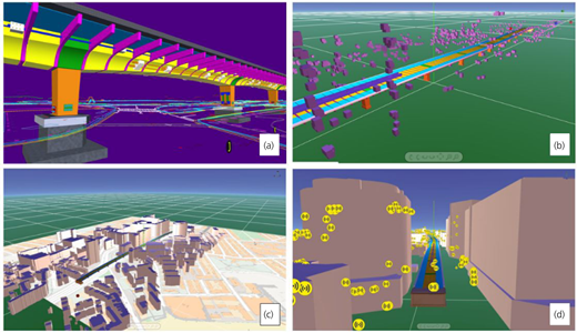
Three-dimensional interpretation of PS points on the Hammersmith flyover: (a) BIM model stripped to pure geometry; (b) bridge model imported into GIS space with PS points; (c) Ordnance Survey building elevation information also imported into GIS space; (d) model and PS in GIS environment used to aid interpretation of PS points
Three-dimensional interpretation of PS points on the Hammersmith flyover: (a) BIM model stripped to pure geometry; (b) bridge model imported into GIS space with PS points; (c) Ordnance Survey building elevation information also imported into GIS space; (d) model and PS in GIS environment used to aid interpretation of PS points
6.2 Method for the identification of target points
The persistent scatterers for Hammersmith flyover are located primarily on either side of the bridge deck, suggesting that the SAR reflections might come from the parapet or outer edge of the concrete deck. There are no points present on the central reservation or roadway. This is logical, as cars, trucks and other vehicles regularly pass over the roadway, preventing the SAR signal from reaching a consistent point. The passing of vehicles could also block SAR reaching the central reservation, which ends up being in a radar shadow at various moments, therefore eliminating persistent scatterers (i.e. steady coherent reflections) in this region too.
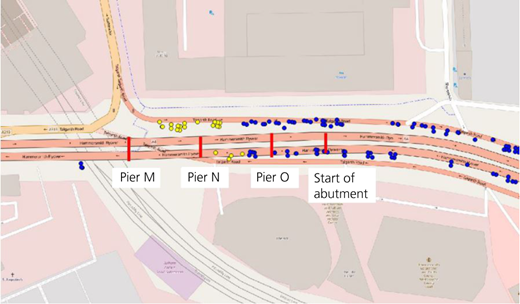
To associate persistent scatterers with the bridge, InSAR persistent scatterer locations were overlaid on the 3D model of the Hammersmith flyover and models of the surrounding building (Figure 8). Persistent scatterers were selected as those within a buffer of a couple of metres of the bridge. The outcome of this selection is shown in Figure 9. To associate persistent scatterers with a specific pier, the authors divided the deck in lines at each midspan, and all persistent scatterers in between consecutive midspan lines were attributed to the pier midway between either line. A number of persistent scatterers attributed to a particular pier (pier N) are shown in yellow in Figure 10. In this diagram, any other persistent scatterers attributed to buildings and other objects have been already excluded by using the 3D models to identify points attributed to objects outside of the bridge.
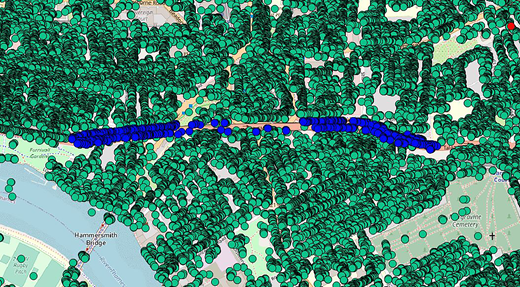
Outcome of the selection process to identify persistent scatterers associated with the bridge (marked in blue) from other persistent scatterers (marked in green). The GCP used in the InSAR processing of the Sentinel data and 2015–2018 Cosmo-SkyMed data is marked in red
Outcome of the selection process to identify persistent scatterers associated with the bridge (marked in blue) from other persistent scatterers (marked in green). The GCP used in the InSAR processing of the Sentinel data and 2015–2018 Cosmo-SkyMed data is marked in red
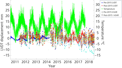
Movement of pier N as measured by an LVDT (two different systems, pre- and post-2015) with temperature and all InSAR PS points attributed to pier N over time. This graph is deliberately difficult to interpret, highlighting the need to identify and select on the PS with the relevant behaviour attributed to the bridge thermal expansion of the bearings. The filtered results are presented in Figure 16
Movement of pier N as measured by an LVDT (two different systems, pre- and post-2015) with temperature and all InSAR PS points attributed to pier N over time. This graph is deliberately difficult to interpret, highlighting the need to identify and select on the PS with the relevant behaviour attributed to the bridge thermal expansion of the bearings. The filtered results are presented in Figure 16
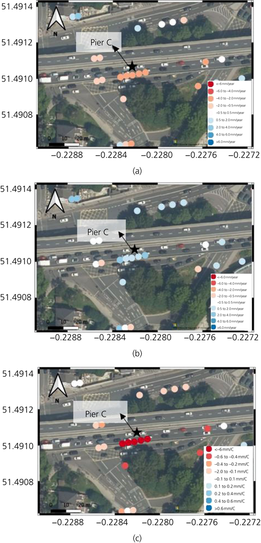
(a) Average velocity map using InSAR Sentinel results for LOS measurement at pier C; (b) same velocity map with the thermal dilation parameter in LOS; (c) average thermal dilation parameter for these same scatterers. All results using ascending Sentinel-1 images between November 2015 and October 2017 and the deformation and time series for the pier C PSs are seen in Figures 13 and 15
(a) Average velocity map using InSAR Sentinel results for LOS measurement at pier C; (b) same velocity map with the thermal dilation parameter in LOS; (c) average thermal dilation parameter for these same scatterers. All results using ascending Sentinel-1 images between November 2015 and October 2017 and the deformation and time series for the pier C PSs are seen in Figures 13 and 15
Combining the knowledge of this behaviour with the measured temperature over several years would suggest that the bridge would expand and contract in an oscillation on a daily basis (which would not be captured by the frequency of SAR acquisitions) and show an oscillating motion in the piers on an annual basis as they respond to the warmer summer months and colder winter months. This expected oscillating movement in the piers was confirmed by displacement gauge data collected from the base of each pier, which showed the horizontal movement of the bearing in the form of a sinusoidal oscillation over a yearly period. Therefore, the persistent scatterers of interest from the bridge (those that reflect the movement accommodated through the bearings) were those with a sinusoidal profile.
Of the persistent scatterers assigned to the pier, identified using the digital models, not all of the points reflect the behaviour described. Figure 11 shows the time series results for pier N. It should be noted that the LVDT measurements are taken at the base of each pier and measure movement in the bridge longitudinal direction, while the InSAR measurements are displacements measured in the LOS of the satellite. From Figure 11, it is not possible to discern which scatterers pertain to the thermal expansion movement of the bridge directly.
To search and identify the persistent scatterers of interest that exhibit an oscillating behaviour (to target those that represent the seasonal motion of the piers), the authors employed Fourier transformation. Specifically, the method employed makes use of the fast Fourier transform (FFT). Fourier transforms are used to decompose a function of time into the frequencies that it is composed of – that is, it is the frequency domain representation of the original signal.
The time-dependent signal as an expansion of its frequency components, or the Fourier transform F(ω), is represented as a signal f defined for all t as follows:
The discrete Fourier transform (DFT) is version of the Fourier transform that deals with a finite discrete-time signal and a finite or discrete number of frequencies. The FFT is another method for calculating the DFT based on the size of the input data being a power of 2 and is computationally many times more efficient than the DFT (the complexity of computing being reduced from O(N 2) to O(N log N), where N is the data size (Van Loan, 1992). Passing the data through a DFT reveals the number of different sine wave frequencies that sum together to form the considered signal. Therefore, passing the time series measurement of each persistent scatterer that oscillates seasonally reveals clear spikes in the frequency domain (either clearly or with some noise) at low frequencies.
Each persistent scatterer time series for a given pier was analysed in this way. Those that did not show a sinusoidal behaviour were discarded from the considered set. These selected points were then plotted over time against the movement measured by traditional in situ displacement gauges attached to the bearings and bearing pit. The results of this process as conducted for different piers are presented in the following sections. Pier C is presented in Section 7, and the filtered version of Figure 11 for pier is presented in Section 8), which highlights a possible practical use of remote InSAR monitoring in such bridge structures. Not all of the persistent scatterers attributed to the bridge through the 3D model approach are used using this approach but may be useful to review for other behaviours (e.g. settlement, as previously mentioned). In this case, the authors know from structural analysis that the primary motion of the bridge is thermal expansion, and the authors are developing a means of targeting these persistent scatterers, which are not immediately obvious within the wider data set.
7 Validation of InSAR measurements using in situ measurements
In this section, the agreement between the InSAR results and the ground-based measurements for Hammersmith flyover is evaluated. As discussed in Section 3, LVDT data are available for each pier of the Hammersmith flyover. For validation of InSAR data, the authors focus here on pier C, which is the second pier in the bridge from the west-to-east direction, and select the corresponding selected InSAR scatterers attributed to that pier.
Thermal expansion and contraction show a linear correlation with the temperature of the bridge at the time of measurements (Webb et al., 2014). This strong thermal effect can affect the results of the InSAR processing, as it makes ‘unwrapping’, the separation of the φ from the Nλ + φ phase measurement, more challenging. This is because the order of magnitude of measurements is a few centimetres, which is a similar order of magnitude of a single cycle of phase (the wavelengths being 5.6 cm for Sentinel-1 and 3.1 cm for Cosmo-SkyMed), with some persistent scatterers in the image impacted by thermal expansion and others not. The thermal dilation parameter, k, can be estimated by fitting a linear regression to the LVDT deformation measurements according to the following equation:
where ΔD and ΔTemp are the measured LVDT deformation difference and recorded temperature difference between each measurement date and the reference date. The temperature sensor recorded data at span BC every 15 min from November 2015 to October 2017.
LVDT deformation data are available at each time that the temperature is recorded.
To estimate the thermal dilation parameter from InSAR measurements, the recorded temperatures at the acquisition date and time of each satellite image needed to be found. Moreover, the phase equation (used to describe the phase measurement described in Section 2.2) is made up of a number of components in addition to the actual motion component. These include a topographic component, the difference in atmospheric propagation between acquisitions, the error introduced due to the use of imprecise orbits in mapping the contributions of Earth’s ellipsoidal surface and noise. For this work, the phase equation used in the standard InSAR processing within the StaMPS processing software was modified to account for the thermal dilation component of movement. The modified phase equation is defined as follows:
where is the unwrapped phase of pixel i in the interferogram j, λ is the radar wavelength, vi is the velocity of pixel i, ΔTj is the temporal baseline of the interferogram j, ki is the thermal dilation parameter for pixel i, ΔTempj is the temperature baseline of interferogram j that is the temperature difference between primary and secondary images and is the residual phase. vi and ki are the two unknowns for pixel i. Figure 12 show the results of this process for pier C, which also confirms that the motion of the bridge is primarily driven by temperature. Removing the thermal component showed no other sources of bridge deformation, as measured by the satellite.
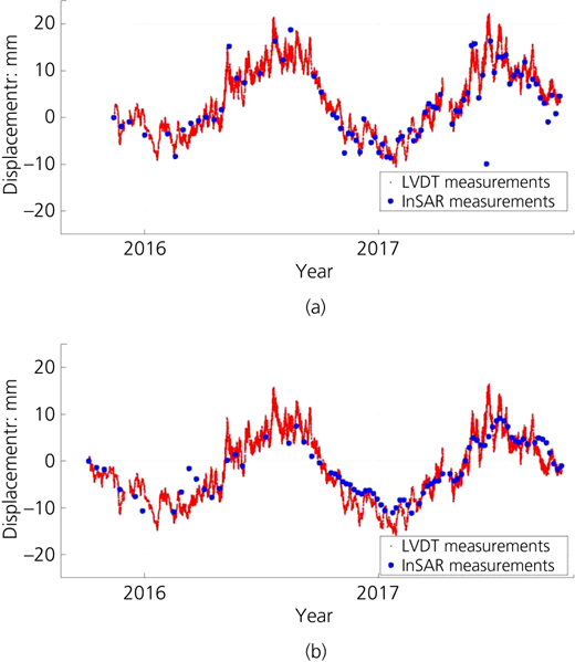
Time series of LVDT displacement at pier C plotted against (a) ascending and (b) descending Sentinel-1 InSAR data for PS located at pier C. For the InSAR measurements, the LOS displacement measurements have been converted into the component of the measurement that is in the horizontal direction parallel to the bridge, so that the InSAR measurements can be directly compared with the LVDT measurements
Time series of LVDT displacement at pier C plotted against (a) ascending and (b) descending Sentinel-1 InSAR data for PS located at pier C. For the InSAR measurements, the LOS displacement measurements have been converted into the component of the measurement that is in the horizontal direction parallel to the bridge, so that the InSAR measurements can be directly compared with the LVDT measurements
Given that the LVDT measures the horizontal linear deformation along the longitudinal direction of the bridge, to compare InSAR deformation data with movements measured by the LVDT, the longitudinal component of the LOS measurement in parallel orientation to the bridge must be found. Equation 3 estimates the magnitude of the horizontal deformation along the bridge from InSAR LOS deformation as follows:
where
and is the range change in the LOS direction; û is the unit vector along the bridge; Î = [Ie, In] is the horizontal unit vector in the satellite LOS direction; Φ is the angle of the bridge with the north direction in the horizontal plane; and θ and α are the incidence and ground heading angles for the selected pixel, respectively.
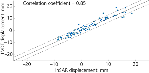
Figure 13 shows the time series of LVDT movement data for pier C plotted alongside the time series of InSAR deformation along the bridge for the corresponding selected InSAR pixel. The temporal and spatial references are defined as the first common date and a stable area close to the bridge (within 2 km of any point of the bridge). These comparison of results from ascending and descending data sets in this specific example of the Hammersmith flyover (e.g. Figure 13) show good agreement between the LVDT and InSAR, even with different satellite viewing geometries. This indicates that the two geometries are independent, which in this particular example occurs because the motion of the bridge was 1D in a nearly east–west direction. This may not be true in other bridge-monitoring applications, and the decomposition into horizontal and vertical displacements may be more complicated (e.g. Selvakumaran et al., 2020) but extremely relevant to consider.
LVDT deformation against InSAR deformation estimated using Sentinel-1 data. The black solid line marks the y = x axis (perfect correlation); the dashed black lines mark the confidence bounds (1σ = 3 mm) assuming that the standard deviation of differences between the two data sets equals 3 mm
LVDT deformation against InSAR deformation estimated using Sentinel-1 data. The black solid line marks the y = x axis (perfect correlation); the dashed black lines mark the confidence bounds (1σ = 3 mm) assuming that the standard deviation of differences between the two data sets equals 3 mm
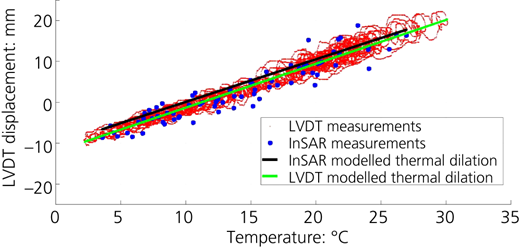
Plot of LVDT data and converted StaMPS InSAR data along the bridge against recorded temperature and the fitted linear trend to them. The estimated thermal dilation parameter is the slope of the plotted line
Plot of LVDT data and converted StaMPS InSAR data along the bridge against recorded temperature and the fitted linear trend to them. The estimated thermal dilation parameter is the slope of the plotted line
Correlations between the converted InSAR deformation data along the bridge and LVDT deformation data are plotted in Figure 14. Figure 15 plots the deformation along the bridge measured by InSAR and LVDT against recorded temperature and shows the fitted linear trend to the data by each method used. The estimated thermal dilation parameter is the slope of the plotted line, which is 1.07 mm/°C for LVDT data and 1.04 mm/°C for InSAR Sentinel data. This confirms that the in situ measurements agree with the InSAR measurements (of a different viewing geometry) and the thermal dilation parameter can be estimated using either sets of measurements.
Points representing persistent scatterers associated to the bridge overlaid onto a map of the bridge. The points in yellow highlight persistent scatters on the south side of the bridge that were attributed to pier N. The points in blue are other persistent scatterers attributed to the bridge
Points representing persistent scatterers associated to the bridge overlaid onto a map of the bridge. The points in yellow highlight persistent scatters on the south side of the bridge that were attributed to pier N. The points in blue are other persistent scatterers attributed to the bridge
8 Detecting potential bridge bearing problems
To study the behaviour of the Hammersmith flyover, both Sentinel and Cosmo-SkyMed data sets were processed. The PS can be visualised with linear velocities marked by colour (as described in Section 5), which would identify issues such as settlement of the bridge or ground in the vicinity of the bridge, but there are also other potential bridge behaviour problems that would not be flagged by visualising the velocity of the PS, but could be studied for early warning. Oscillating behaviour, as presented, would suggest no motion when studying a velocity map. Given the finer spatial resolution of the Cosmo-SkyMed data and resulting higher density of scatterers on the bridge, these data were used in this section to study anomalies in bridge thermal expansion behaviour, which can indicate problems with bearings and expansion joints.
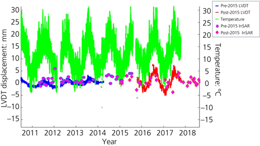
Movement of pier N as measured by LVDT (two different systems, pre- and post-2015) and two selected InSAR PS points (with 2011–2015 data set and 2015–2018 data set), alongside temperature. This plot shows a change in the amplitude of oscillation in both LVDT and InSAR measurements from the period prior to 2014 and the period after 2015, which indicates a structural change in the bridge in that the bearings are able to move more freely and facilitate the bridge thermal expansion
Movement of pier N as measured by LVDT (two different systems, pre- and post-2015) and two selected InSAR PS points (with 2011–2015 data set and 2015–2018 data set), alongside temperature. This plot shows a change in the amplitude of oscillation in both LVDT and InSAR measurements from the period prior to 2014 and the period after 2015, which indicates a structural change in the bridge in that the bearings are able to move more freely and facilitate the bridge thermal expansion
The authors’ method provides a means of selecting InSAR points that exhibit an oscillating behaviour over time. Monitoring for changes in the nature of this oscillating behaviour can then be used to spot signs of unusual behaviour in the Hammersmith flyover. After a period of monitoring and assessment, the bridge was found to have problems with some of its bearings. In particular, some of the bearings were found to have seized, severely restricting horizontal movement of the bridge at the pier locations of these seized bearings (Webb et al., 2014). To address this issue, bearing replacement activities were carried out in 2014 and 2015.
In the case of seized bearings, such as pier N (presented in Figure 11), the LVDT readings show the bridge expanding and contracting to a much larger extent after the bearing replacement – that is, the post-2015 LVDT readings have a much larger amplitude of oscillations than the pre-2015 LVDT readings. The authors applied the FFT method outlined to each of the persistent scatterers plotted in Figure 11 to select oscillating points of interest. The selected persistent scatterers of interest (showing oscillations) are shown in Figure 16. The motion of pier N corresponds to the temperature, also plotted in this figure using readings taken from sensors installed through the bridge deck in the midspan between piers O and P. In this figure, the motion prior to 2014 for both LVDT and InSAR measurements has a lower amplitude than the movement measured after 2015, indicating structurally that the bearings are able to move more freely after 2015 to allow the bridge deck to expand and contract with temperature more freely (as the seized bearing was replaced between 2014 and 2015).
Using structural modelling and understanding of the bridge behaviour, the primary cause of deformation of the Hammersmith flyover was found to be thermal loading, which causes expansion and contraction in the longitudinal direction of the bridge, with most movement occurring in the centre of the bridge and decreasing towards each span. A structural finite-element model of the Hammersmith flyover was used to model a series of different loading and temperature scenarios. The movement of the bridge was proportional to the thermal load, as also described by more detailed studies of the flyover, such as that by Webb et al. (2014).
Ideally, this study would have shown the results of InSAR and LVDT measurements before and after bearing replacement of a pier towards the centre of the bridge with a seized bearing. The piers towards the centre of the bridge experience much larger horizontal displacements (and therefore larger amplitude of oscillations). However, none of these piers had bearings that seized. Pier N was known to have had a bearing that seized and was replaced in 2014/2015, as it had a much smaller amount of horizontal displacement than more central piers. It is less easy to see the difference in oscillation amplitude before and after the bearing replacement.
This case study is used to show the potential of using InSAR to spot the unusual movement behaviour of bridge assets. In practice, this would not be a clear step change in behaviour as shown here from seized to free-moving bearing. In cases such as Hammersmith flyover, the amplitude of oscillation over time is unlikely to be a sudden change but a slow reduction of movement over time. This would be less straightforward to identify but could be seen in InSAR measurements collected regularly over a period of years starting from before the problems began.
9 Discussion
In terms of the application of SAR to bridge monitoring in practical terms, not only SAR data can not only be used in the absence of other sensor measurements (in this instance to spot unusual or anomalous behaviours), but they can also be used to augment the information provided by a wider digital sensor network. However, these must be taken with an understanding that SAR measurements are not useful in all bridge-monitoring cases and will not provide useful measurements for all bridges and applications. These considerations are presented in the following discussion.
9.1 Understanding the suitability of InSAR for monitoring a specific bridge
To understand whether InSAR monitoring is suitable for a specific case requires the end user to have a clear idea of what the measurement goal and requirements are. This means understanding what kind of bridge movements are expected, including direction and maximum movements. This needs to be considered against what the satellite can realistically capture given its wavelength, spatial resolution and pixel size. The imaging and processing of SAR images limit the types of deformation that can be monitored. As mentioned, using a SAR sensor in a specific wavelength of the electromagnetic spectrum limits the movements that can be unambiguously defined to measurements of (λ/4) or less between acquisitions. In cases of monitoring settlement and deformation of ground over wide areas, this also sets a maximum differential deformation rate.
The end user must also have an understanding of SAR viewing geometry. This includes the LOS measurement direction, relative nature of the measurement and the implications of having a side-looking sensor on a satellite travelling in a north–south direction. The direction of horizontal displacement for the Hammersmith flyover is the east–west direction. This is ideally orientated for SAR viewing geometry to pick up horizontal displacements between acquisitions, but the same bridge in a north–south orientation would not yield the same results. Given that the Hammersmith flyover is known to have negligible vertical displacement at the piers (from previous studies such as that of Webb et al. (2014) as well as viewed in the monitoring data itself), the InSAR LOS measurement would primarily be picking up the horizontal thermal expansion. However, generally speaking, this form of InSAR measurement is a 1D measurement in an arbitrary direction to the bridge. InSAR measures the component of 3D motion that occurs in the LOS of the satellite.
There are methods in the literature for deriving 3D components (Wright et al., 2004), but this requires different satellite look directions on the same point. In practice, it is difficult to achieve readings at the same point on bridges and some significant assumptions need to be made to do so. This is explored using the Waterloo Bridge as a case study in the study by Selvakumaran et al. (2020).
Although remote sensing provides the advantage of covering wide areas, it may not be suitable for all bridges in a given area and may require a tailored approach to each site within an image. Another consideration is whether the bridge to be monitored sufficiently reflects SAR waves and whether measurements can be collected at the points/regions of interest. There are different processing algorithms available, depending on the reflective behaviour to be monitored. Many bridges studied in the literature employ some variation or development of PSI. In instances where the bridge does not have dominant scatterers, but instead a more distributed signal, other methods such as SBAS can be employed (e.g. the masonry bridge studied by Selvakumaran et al. (2018)). In some cases, the bridge could have corner reflectors installed to augment the reflection response (e.g. Selvakumaran et al., 2020). The installation of corner reflectors was also considered for this study, to induce persistent scatterers at points in a known geographical region, but in practice, it was not possible to have them installed. Initially, the side of the parapet was considered, but they could not be installed at that location due to a manufacturer’s warranty, which would be declared invalid for the parapet if anything was attached to it. The central reservation and top of the parapet were also discounted from consideration for fear of causing distraction to drivers. Finally, the side of the bridge itself was considered. This was permitted but would require road closures and the rental of lifting machinery to reach a suitable installation height, which would incur too much cost. Checking the reflectivity of a bridge could be done by looking at radar images, test processing or using radar simulations (Auer, 2011; Auer et al., 2010) to understand SAR viewing geometry better.
Linked to this point is the work outlined in this paper related to interpretation. The opportunistic nature of InSAR measurement may not suit single asset monitoring in some cases but, conversely, may provide insights into the ground behaviour in the environment of the asset. As shown using the example of the Hammersmith flyover, there is an element of interpretation that is more nuanced and complex than reading the output from sensors and surveying that the civil engineering community is familiar with.
9.2 Understanding InSAR data quality
It is important for asset managers using InSAR-derived products to understand some of the influences from noise, acquisition and processing that contribute towards resolution and measurement quality. In practice, there are a number of methodology choices and parameters that are chosen during the processing that affect the measurement output. Skill is needed in understanding the impacts of these choices, as well as in understanding and identifying key impacts, such as atmospheric artefacts or effects due to perpendicular baselines. For further resources on the topic of understanding InSAR time series data quality, see the publications by Ferretti et al. (2007b) and Sadeghi et al. (2021).
9.2.1 Number of images
There is a minimum number of SAR images required for PSI. This is informally acknowledged to be 20–25, with a preference for more images if possible. Having a larger stack of images available does not just give more dates for measurement readings in the end product but also allows for better atmospheric and orbital error correction. Using too few images can increase the noise and measurement uncertainty of readings. The spacing and frequency of images also have an impact on the results, such as large gaps in the time series. Thus, when planning the collection of images or looking up archive images, it is worth noting that this cannot be achieved with just a handful of images.
9.2.2 Image resolution
End users of the SAR data should note that the SAR image resolution in the raw data will be finer than the resolution of the processed images and resulting measurements. In this paper, the effects of imaging geometry, the projection from SAR coordinates to geographic coordinates and multi-looking (averaging of pixels) during processing are discussed and some explanations as to why this is the case are provided.
9.2.3 Reference points
Reference or control point(s) are locations where there is assumed to be no motion or with a known motion. The measurements of persistent scatterers are calculated relative to these control points. This is analogous to setting up an automated total station to read measurements relative to the measurement of a reference prism positioned in a location that is assumed to be stable and without motion. In both cases, there is the potential to introduce some error if reference points are selected that are also moving. Generally, it is recommended that the reference point be close to the site being studied. There is an increasing likelihood of changes in atmospheric conditions moving further away from the target site, which results in an increase in atmospheric noise contributing to the signal measurement.
9.2.4 Coherence values
Coherence is used as a measure of change between acquisitions (for a number of reasons in addition to temporal change, such as noise and atmospheric effects). The coherence value for a particular pixel used as a scatterer can be used as a measure of data quality in selecting the most appropriate scatterers to study. These values range from 0 (completely decorrelated) to 1 (perfect coherence).
9.3 Deploying InSAR for bridge monitoring
For the civil engineering sector to consider the incorporation of InSAR technologies into monitoring strategies, there is significant value in being an educated user and building experience within organisations, but it is worth considering such monitoring as a specialism that requires a level or training and expertise or the engagement of specialist providers.
As highlighted throughout this study, there are a number of aspects to consider when deciding whether InSAR is appropriate for a particular project. Considerations include the bridge geometry, material, orientation and direction of movement to be measured. There is also the opportunistic nature of measurements, which rely on how the asset and its surroundings reflect radar at the imaging moment; preliminary work should be done using archived imagery to investigate feasibility.
In a similar analogy to the creation of finite-element models for structural understanding of bridge behaviour, the implications of various assumptions and parameters selected during InSAR processing can have a significant impact on the measurements calculated. Despite a number of simple-to-use software packages developed in recent years, there is a risk in allowing users to plug in parameters without understanding the impact, similar to someone creating a bridge model without understanding structural behaviour and the assumptions built within finite-element method packages. For that reason, it is advisable that the processing of SAR data be undertaken by an InSAR processing specialist (and there a number of specialist companies that undertake this work).
10 Conclusions
Satellite-based InSAR technology can be effectively implemented for long-term bridge deformation monitoring with millimetre-scale precision, augmenting conventional inspection methods with more frequent movement measurement readings. The results of InSAR monitoring of the Hammersmith flyover, performed between 2011 and 2018, provide evidence that InSAR can be used to monitor bridge expansion due to seasonal thermal variation. The results show that InSAR monitoring can be deployed remotely to monitor and spot unusual bridge movements. In this paper, this was demonstrated by spotting change in bearing movement behaviour in the Hammersmith flyover. This included the development of a method for isolating the specific signal of interest (derived using bridge modelling and understanding) from other effects. In doing so, the opportunity to integrate 3D modelling and BIM systems with satellite data and GIS systems to interpret satellite measurements better from an end-user perspective was highlighted.
Acknowledgements
The authors would like to thank Transport for London for providing access to monitoring data and archive information, with special thanks to Peter Jones and Nicola Head. The authors would also like to thank Group BC and PCSG (particularly Mark Bew and Sanjeev Shah) for their support, input and access to their GeoConnect+ platform. Thanks also go to Ramboll for providing their BIM models and structural modelling data.
Access to Cosmo-SkyMed X-band SAR data for 2015–2018 was provided by the Satellite Applications Catapult under the Italian Space Agency Cosmo-SkyMed Radar Science and Innovation Research programme and the processed sets of InSAR PSI results for 2011–2015 were provided by Telespazio. Sentinel-1 data were obtained through the Copernicus programme of the European Space Agency.
This research forms part of Centre for Digital Built Britain’s (CDBB) work within the Construction Innovation Hub. The funding from CDBB was provided through the government’s modern industrial strategy by Innovate UK, part of UK Research and Innovation. This work also received funding from Engineering and Physical Sciences Research Council (UK) Award 1636878, with iCase sponsorship from the National Physical Laboratory, as well funding from the Isaac Newton Trust. Research was also conducted as part of Comet, the Natural Environment Research Council’s (NERC) Centre for the Observation and Modelling of Earthquakes, Volcanoes and Tectonics, a partnership between UK universities and the British Geological Survey.

