


The purpose of this study is to conduct a critical review of the operational and financial trends of Uttar Haryana Bijli Vitran Nigam Limited and Dakshin Haryana Bijli Vitran Nigam Limited. Furthermore, the study aims to determine whether loss-making utilities would benefit from adopting the strategic model employed by Haryana.
Time series data from 2005–2006 to 2022–2023 is analysed using various significant accounting ratios and operational and financial performance parameters to assess the annual performance over the period.
The substantial operational and financial performance results of UHBVNL and DHBVNL indicate that from 2017 to 2018 onwards, the power discoms started performing well and are in an improving stage. These results create a strong profile for the utilities, suggesting that their model could be a viable solution for other loss-making power distribution companies.
As a policy recommendation, rather than privatizing the discoms, authorities should study the strategic model of profit-making states like Haryana and implement it in other states without any political interference.
The relevant research questions addressed are: What best practices have Haryana power discoms adopted to enhance financial performance and minimize losses? What lessons can other loss-making state-owned power discoms learn from Haryana? Can Haryana power discoms be a benchmarking model for public and private discoms operating at a loss?
1. Introduction
Sustainable economic growth in India puts immense pressure on energy and infrastructure services. India is one of the world’s biggest energy markets, equivalent to the electricity networks of the European Union, China, Russia and the United States (IEA-India, 2021). In the entire value chain of the energy sector, the distribution utilities are considered a cash register and a vital link. Power distribution utilities collect revenues from users for their power supplies to provide the generation and transmission sectors with the required cash flows to operate. Due to consumers' payment delays, generators do not receive timely payments from the distribution companies (discoms), which places a burden on the generators (Keeley & Keeley, 2016; Emon, 2021; Singh & Vashishtha, 2021). This deficit is covered by financing, government subsidies and potentially a reduction in spending. In return, it raises the borrowing cost of discoms (interest), which is inevitably borne by consumers. It undermines the capacity of the discoms to purchase and distribute electricity to meet their Universal Supply Obligation (Nirula, 2019; Shankar & Avni, 2021).
Electricity distribution in India is one of the weakest segments of the power sector’s value chain. Electricity distribution utilities are suffering under considerable debts to the thermal power stations. Over US $100bn of stranded assets are shared by distribution utilities and coal and gas-fired power plants. There is an increase in discoms’ losses on a subsidy-received basis, accumulated losses as per the balance sheet, outstanding dues by discoms and total outstanding debt (Pandey &Ghodke, 2019; Garg & Shah, 2020). At present, 55 power distribution utilities in 36 States/Union territories exist in India. Most of the States/Union territories have one distribution utility except Gujarat, Haryana, Karnataka, Uttar Pradesh and Odisha. Rajasthan has the highest profit amount of 2,986 Crore, followed by Delhi, West Bengal and Gujarat, respectively. In contrast, the discoms in Tamil Nadu have the highest loss amount of 11,965 Crore, followed by Andhra Pradesh, Telangana and Madhya Pradesh, respectively. Surprisingly, 66.67% of States/Union territories (24 out of 36) were operating at a loss, while only 33.33% were in profit (PFC, 2020).
After gaining independence in 1947, India started a series of policies and plans to improve State-Owned utilities’ operations and financial health (Swain, 2016; CEA, 2018; Veluchamy, Sunder, Tripathi, & Nafi, 2018). Their success has been limited despite these measures and the distribution sector remains a source of drain on the Indian economy. Despite India’s excellent steps in strengthening its power generation and transmission capacity throughout the past few years, the nation lags in distribution. However, unless the distribution sector becomes powerfully revamped, there is a risk that additional power generation and transmission assets will become stranded, delaying much-needed additional investment and technological growth. To fulfil its magnificent renewable objectives and strengthen its economic growth objectives, the financial stability of discoms is essential (Sarangi, Mishra, Chang, & Taghizadeh-Hesary, 2019; Zhu & Liao, 2019). The poor financial health of the discoms implies that these utilities struggle to pay for electricity generators and frequently fail to comply with their agreements, which impairs their capability to invest in modern technologies and revitalize the power station.
The Indian federal system comprises several States (Haryana is one of them and the study’s geographical focus area) and developing policies for the entire country is somewhat different from doing so for a single State. The economic viability of the electricity sector has gained significant relevance since it is critical to have comparable data at the aggregate level to formulate appropriate policies to accomplish the nation’s significant growth target (Singh, 2021). Considering the need of the hour, the current study analysed the performance of Haryana power distribution utilities and aims to answer, “Can Haryana power discoms be a benchmarking model for other public and private discoms running into losses?” Consequently, an endeavour was undertaken in this study to analyse Haryana Power Utilities’ (HPUs) performance. Although the study focused on a single region, the adopted practices are replicable across the country, providing a unit-by-unit perspective of a relatively complicated environment in a vast country like India.
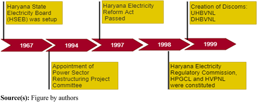
The process of reform of the power sector was initiated in the early 1990s in India. After Orissa, Haryana was the second State to undertake reforms in the power sector (Gurtoo & Pandey, 2001; Zhang, 2008). The reform process was facilitated in the direction of the World Bank. In 1994, the National Economic Research Associates (NERA) of the United States undertook the Haryana Power Sector Restructuring project (Haryana Government Gazette Extraordinary, 1998). The Haryana State Electricity Reform Bill, 1997 was passed on 22nd July 1997. The Act provides for the establishment of the Electricity Regulatory Commission, the restructuring of the electricity industry and the rationalization of the generation, transmission, distribution and electricity supply (Planning Commission, 2000). In 1999, two distribution companies had been formed for distribution and retail supply: Uttar Haryana Bijli Vitran Nigam Limited (UHBVNL) and Dakshin Haryana Bijli Vitran Nigam Limited (DHBVNL). Figure 1 illustrates the chronology of power sector reform measures in Haryana.
Electricity is a fundamental element and is widely recognized as the backbone of the economy. The HPUs were financially weak and ran into huge losses even after various measures. These measures included capacity addition plans, considerable investments to change aging plants and machinery, encouraging private players to participate and implementing the Restructured Accelerated Power Development and Reforms Program (Kaur & Chakraborty, 2018; Bhardwaj & Sharma, 2020). However, the financial health of the utilities was still unsound. Therefore, several schemes were initiated by the state and central government to boost the infrastructure of distribution and assist the discoms in enhancing their economic viability. Some of these schemes include Ujjwal Discom Assurance Yojana (UDAY), Deen Dayal Upadhyay Gram Jyoti Yojana (DDUGJY) and Integrated Power Development Scheme (IPDS) (Agrawal, Kumar, & Rao, 2017; Saha, 2018). Despite these initiatives, a sustainable turnaround of the discoms was not assured.
The Power Financial Corporation (PFC) authorized Credit Analysis & Research Ltd. (CARE) rating agency to grade and rank power discoms. The integrated ranking report of Haryana power discoms in 2021, 2022 and 2024 is presented in Table 1. The CARE agency ranked both discoms with a higher rating of A and A+. Considering the need of the hour, the current study critically reviews and explores the best practices used by Haryana power discoms for improving financial performance and reducing losses. The addressed research questions are: What best practices can other states adopt to improve the economic health of their power discoms? What lessons can other loss-making state-owned power discoms learn from Haryana? Can Haryana power discoms be a benchmarking model for other public and private discoms running into losses?
Rank and grade of Haryana power discoms
| Ranking year | Rank | Discom | Grade* |
|---|---|---|---|
| 2021 | 5th | Dakshin Haryana Bijli Vitran Nigam Limited | A+ |
| 6th | Uttar Haryana Bijli Vitran Nigam Limited | A | |
| 2022 | 9th | Dakshin Haryana Bijli Vitran Nigam Limited | A+ |
| 10th | Uttar Haryana Bijli Vitran Nigam Limited | A+ | |
| 2024 | 11th | Uttar Haryana Bijli Vitran Nigam Limited | A+ |
| 12th | Dakshin Haryana Bijli Vitran Nigam Limited | A+ |
Note(s): Grade* – A+: Very High Operational and Financial Performance Capability; A: High Operational and Financial Performance Capability
Source(s): Table by authors
The rest of the study is organized as follows: literature is discussed in Section 2. Methodology and results are presented in Sections 3 and 4, respectively. Finally, conclusions and policy implications are recommended in Section 5.
2. Empirical literature
The challenges faced by power distribution utilities in India have been extensively documented in the existing literature. From time to time, researchers shed light on the economic and financial constraints of discoms. Alam, Kabir, Rahman, and Chowdhury (2004) investigated the reform initiatives and the scenario in Bangladesh’s power distribution system. Based on the study, the authors asserted that priority must be given to the distribution system instead of generation and transmission because the distribution system was characterized by heavy system loss and poor collection performance. Abhyankar (2005) investigated the financial and operational performance of the Madhya Pradesh State Electricity Board (MPSEB) from 1993 to 2004. In a nutshell, due to poor financial performance and a credibility crisis, the MPSEB became financially fragile. Small consumers also remained burdened with considerable tariff increases, and the State government with subsidies. Ranganathan (2005) compared the Transmission & Distribution (T&D) losses of three states, namely Karnataka, Andhra Pradesh and Tamil Nadu, for 2002–2003 and the measures to be adopted by both public and private sector utilities for reducing the losses. The author suggested that the power sector should use load flow analysis, physical enumeration, meter reading, non-hookable wires and revenue monitoring.
Bhattacharyya (2007) investigated the challenges and issues faced by the power sector in India. The author identified several challenges, including coordinating global influences, resource management, effects of price shocks, energy supply security, financial difficulties, budget constraints and unfinished reforms. Oseni (2011) analysed the Nigerian power sector’s performance and presented policy recommendations for establishing a global power market and ensuring environmental sustainability. The study concluded that the Nigerian power sector faced severe issues such as low maintenance and management, equipment theft, insufficient power investments, lack of competition and corruption. Dhara, Sethia, and Chitkara (2014) examined the performance of power discoms in 20 central Indian states over the years 2006–2010, applying input-minimizing Data Envelopment Analysis to cross-sectional and time-varying data. The study results indicated that the performance of numerous discoms was sub-optimal, indicating a possibility for cost savings and a decrease in energy losses.
Azhar (2015) studied the effect of liquidity and management efficiency on the profitability of India’s superior power distribution utilities. The study revealed that the debtor’s turnover ratio, collection efficiency and interest coverage ratio significantly impacted profitability. In contrast, the quick ratio, absolute liquid ratio and creditor’s turnover ratio demonstrated an insignificant impact on profitability. Keeley and Keeley (2016) investigated the case study of NTPC and Rajasthan power distribution utilities to highlight various methods to improve financial and operational efficiency. The financial stress and AT&C and T&D losses were very high in the states from 2010–11 to 2014–15. The authors concluded that a strong bond and cooperation between the Centre and State governments is required to successfully implement the new financial bailout scheme. Ojha (2018) examined the factors influencing the Indian power sector’s performance and focused on states’ performances under the UDAY scheme. The author attributed high AT&C losses, low tariff rates, political interference, power thefts, lack of technical regulation mechanisms and inaccurate metering as reasons for low performance.
Singh and Vashishtha (2019) assessed the performance of Haryana discoms on the financial and operational parameters of Ujwal Discom Assurance Yojana (UDAY) from 2015–16 to 2018–19. The study results showed insignificant growth in the DT meter (Rural), smart metering above 500 KWH and intelligent metering between 200 and 500 KWH parameters. Veluchamy, Sunder, Tripathi, and Nafi (2020) examined the financial and operational performance of the Indian energy distribution industry and the UDAY framework’s effect from 2016 to 2019. The researchers concluded that while the UDAY scheme led to significant achievements in operating parameters and the recognition of discom debts by State governments, the intended outcome of making discoms financially and commercially viable was not achieved. Maurya (2020) presented an overview of the effect of power sector reforms on the operational and financial efficiency of Uttar Pradesh’s power sector utilities. The author concluded that State power utilities still have a long way to go to become financially and economically viable. However, since 2012–2013, the positive effect of the reform initiatives has been abundantly evident.
Kathuria (2021) constructed a reform index and employed data from 55 power utilities across 29 Indian states for the period 2007–08 to 2015–16 to assess the impact on financial and technical-cum-commercial performance. The results showed a wide variation in reform status and performance across utilities, with those implementing more reforms performing better financially, but not technically. Singh and Robita (2022) measured the financial performance of four state-owned Gujarat distribution companies using the DuPont model. The study found that the liquidity position of all four discoms was low, and they maintained very low receivable days over five years compared to the national average. Sharma, Paul, Jha, and Kulkarni (2023) analysed the UDAY scheme parameters and their significant impact on improving efficiency for each power distribution utility. The findings suggest that initiatives under the UDAY scheme helped improve the financial performance, AT&C loss levels and ACS-ARR gap for five discoms. Garg, Mallik, and Raju (2024) explored the critical role of India’s distribution companies (discoms), highlighting the accumulation of operational, financial and political challenges. The authors reported a need for a paradigm shift in the overall functioning of discoms, focusing on digitalization, smart grids, integrating solar rooftop systems, electric vehicles, and demand-side management programs supported by robust monitoring and evaluation systems.
Based on the extensive literature on the challenges and performance of power distribution utilities in India and other regions, a notable research gap exists in the detailed exploration of successful case studies that offer actionable insights for improving financial performance and reducing losses. While previous studies have identified various economic and operational constraints faced by discoms, such as high AT&C losses, poor collection performance and financial fragility, there is a lack of focused research on specific successful models within India that have transitioned from loss-making to profit-generating entities. The Haryana power discoms present a unique opportunity to fill this gap. By investigating the best practices and strategies employed by Haryana power discoms, this research aims to provide a comprehensive benchmarking model. This model can serve as a valuable reference for other state-owned and private discoms struggling with financial and operational inefficiencies. The potential of Haryana discoms as a benchmarking model has not been thoroughly analysed in existing literature, highlighting the need for this research to address the identified gaps and offer practical and theoretical recommendations for the broader power distribution sector.
3. Data and methodology
3.1 Data
A comprehensive dataset spanning from 2005–06 to 2022–23 was compiled from the annual reports and official websites of various power utilities, including the Haryana Electricity Regulatory Commission (HERC), UHBVNL and DHBVNL. Additionally, data was compiled from reports by the Ministry of Power, World Bank studies on the power sector, the Central Electricity Authority and Haryana Statistical Abstracts. Furthermore, information on the recovery of unpaid bills and line losses was obtained through personal visits to the head offices of HPUs.
3.2 Methodology
The operational and financial performance of power distribution utilities is reviewed using annual time series data, employing descriptive statistics and various significant ratios. The descriptive statistics include the mean, standard deviation, variance and compound annual growth rate (CAGR). The operational performance is measured using aggregate technical and commercial losses, transmission and distribution losses, efficiency in the recovery of bills and the defaulted amount of discoms (see Table A1 in Annexure). Liquidity, asset management, solvency and profitability ratios are calculated for financial performance (see Table A2 in Annexure).
4. Results and discussion
4.1 Operational performance
4.1.1 Average cost of supply and average revenue realization gap
The performance, based on the average cost of supply (ACS) and the average revenue realization (ARR) gap of both discoms, disclosed that UHBVNL had a lower gap than DHBVNL. As shown in Table 2, the ACS-ARR gap followed a fluctuating trend over the study period. From 2009–10 to 2016–17, the gap for UHBVNL was comparatively higher than DHBVNL. However, from 2017–18 to 2019–20, UHBVNL realized more average revenue than DHBVNL. From 2020–21 to 2022–23, UHBVNL continued to realize more average revenue than DHBVNL, maintaining a positive gap. The consistent improvement in revenue realization during these years can be attributed to continued efforts in operational efficiency and regulatory support. The major reasons for the lower gap included the use of more efficient super-critical technology in thermal power generation, improved operational norms in the tariff regulations, customs duty exemption for power generating equipment, segregation of agriculture feeders, and modernization of transmission and distribution devices.
Average cost of supply (ACS) and average revenue realization (ARR) gap (In /kWh)
| Year | UHBVNL | DHBVNL | ||||
|---|---|---|---|---|---|---|
| ACS | ARR | Gap | ACS | ARR | Gap | |
| 2009–10 | 4.62 | 4.03 | −0.59 | 3.52 | 3.17 | −0.35 |
| 2010–11 | 4.30 | 4.16 | −0.14 | 3.94 | 3.29 | −0.65 |
| 2011–12 | 7.82 | 3.18 | −4.64 | 5.88 | 3.56 | −2.32 |
| 2012–13 | 5.52 | 4.35 | −1.17 | 4.76 | 4.10 | −0.66 |
| 2013–14 | 5.55 | 4.86 | −0.69 | 5.13 | 4.34 | −0.79 |
| 2014–15 | 5.41 | 4.75 | −0.66 | 4.90 | 4.68 | −0.22 |
| 2015–16 | 5.70 | 5.55 | −0.15 | 5.49 | 5.32 | −0.17 |
| 2016–17 | 5.86 | 5.77 | −0.09 | 5.40 | 5.41 | 0.01 |
| 2017–18 | 5.94 | 6.07 | 0.13 | 5.28 | 5.32 | 0.04 |
| 2018–19 | 7.97 | 8.07 | 0.10 | 6.51 | 6.55 | 0.04 |
| 2019–20 | 7.39 | 7.50 | 0.11 | 6.58 | 6.62 | 0.04 |
| 2020–21 | 6.73 | 6.95 | 0.22 | 6.23 | 6.42 | 0.10 |
| 2021–22 | 6.84 | 7.18 | 0.34 | 6.63 | 6.69 | 0.06 |
| 2022–23 | 8.11 | 8.23 | 0.12 | 7.70 | 7.94 | 0.04 |
Source(s): Compiled from Annual Reports (2009–2023) of Power Financial Corporation
4.1.2 Aggregate technical and commercial (AT&C) losses, collection efficiency (CE) and defaulting amount from connected and disconnected consumers
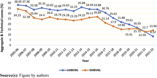
Aggregate technical and commercial (AT&C) loss is a key indicator of a power distribution system’s performance, encompassing both technical and commercial losses. The performance based on AT&C losses reveals that over the period from 2005–06 to 2022–23, DHBVNL consistently maintained lower losses compared to UHBVNL, as shown in Figure 2. In 2016–17, DHBVNL’s losses were 21.14%, gradually decreasing to a minimum of 15.41% by 2019–20. UHBVNL reached a minimum of 19.61% in 2019–20. From 2020–21 onwards, the trend continued with UHBVNL showing a further decrease to 16.55% in 2020–21, 12.7% in 2021–22, and 8.32% in 2022–23. Meanwhile, DHBVNL’s losses fluctuated slightly, with 15.75% in 2020–21, 12.59% in 2021–22, and 13.96% in 2022–23. The UDAY scheme mandated state governments to reduce AT&C losses to 15% by 2018–19 through measures such as mandatory smart metering, distribution infrastructure upgrades and energy-efficient initiatives. These concerns were also highlighted by Veluchamy et al. (2018, 2020) and Kathuria (2021).
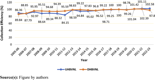
From 2005–06 to 2022–23, the collection efficiency of Uttar Haryana Bijli Vitran Nigam Limited (UHBVNL) and Dakshin Haryana Bijli Vitran Nigam Limited (DHBVNL) has shown notable trends (Figure 3). Initially, UHBVNL started at 89.84% in 2005–06, while DHBVNL began slightly higher at 86.36%. Over the years, both entities implemented measures to improve efficiency. UHBVNL’s efficiency fluctuated, reaching a peak of 100% in 2018–19 and maintaining high levels thereafter, with 99.26% in 2019–20 and increasing further to 102.58% by 2022–23. Meanwhile, DHBVNL’s efficiency saw variations, with a notable peak of 100% in 2017–18, but dropped to 98.78% in 2019–20 and further to 97.8% by 2022–23.
The compound annual growth rate of UHBVNL showed a consistent increase, outpacing DHBVNL, suggesting effective management practices and possibly stricter enforcement against electricity theft and pilferage. Measures such as incentivizing information on theft, promoting prepaid metering and enhancing recovery processes have contributed to these improvements. Effective management practices, including incentivizing reporting of theft and pilferage, adoption of prepaid metering and enhanced recovery processes, have significantly contributed to the improved aggregate technical and commercial (AT&C) performance. As discussed by Bhardwaj and Sharma (2020), Das and Srikanth (2020) and Emon (2021), these measures not only deter electricity theft and material pilferage but also streamline collection processes, thereby increasing overall efficiency and ensuring higher collection rates from electricity users.
Every consumer is expected to make payment of their dues by the “due date.” A consumer who fails to make payment within the given time and does not receive notice of disconnection falls under the “connected consumer” category. On the other hand, “disconnected consumers” are those who fail to settle their liabilities, resulting in possible disconnection of their premises under Section 56 of the Electricity Act, 2003. According to Section 56, a clear fifteen-day notice in writing must be given to such consumers before supply disconnection. Defaulting consumers (both connected and disconnected) are divided into two main categories: private and government. Private category consumers are further divided into domestic urban and rural, non-domestic, industrial and agricultural categories. Government departments include irrigation, public welfare, Municipal Corporations, panchayats and other government departments. The defaulted amounts from government departments (both connected and disconnected categories) were higher for both DISCOMs. However, UHBVNL had a relatively higher default amount from connected consumers compared to DHBVNL, whereas DHBVNL had a relatively higher default amount from disconnected consumers compared to UHBVNL. The defaulted amounts are depicted in Figures 4 and 5.
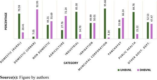
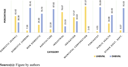
Trend of total defaulting amount from disconnected consumers (as on 31.03.2024)
Trend of total defaulting amount from disconnected consumers (as on 31.03.2024)
The primary reasons for non-payment of electricity bills, including inadequate or irregular consumer incomes, were discussed by Kaur and Chakraborty (2018), Nirula (2019) and Singh and Robita (2022). Discoms had accumulated substantial receivables, primarily due to defaults from various consumer categories, adversely affecting the financial health of utilities. The regulatory commission directs the discoms to conduct an age-wise audit of their receivables and include an action plan to liquidate the outstanding receivables within six months (Section 56, Electricity Act, 2003). Unless a court of competent jurisdiction has granted a stay, the electrical connections of all such defaulting consumers shall be immediately disconnected.
4.1.3 Transmission and distribution losses and billing efficiency (BE)trend
Transmission losses, which represent the discrepancy between the total energy purchased and the actual energy received by distribution companies, have been monitored from 2005–06 to 2022–23 as shown in Table 3. These losses, primarily attributed to power or voltage loss along transmission lines and circuit devices, impact the energy available to distribution companies to meet consumer demand. Notably, DHBVNL consistently recorded lower transmission and distribution losses compared to UHBVNL over the years. From 2008–09 to 2022–23, DHBVNL demonstrated a compound annual growth rate (CAGR) of −2.30%, indicating a substantial decrease in losses, while UHBVNL’s losses decreased at a CAGR of −2.50%. This trend continued from 2020–21 to 2022–23, during which both entities demonstrated further reductions in transmission losses. DHBVNL maintained a technological edge in circuit devices to effectively manage and minimize these losses. Maurya (2020) and Shankar and Avni (2021) noted that consistent reductions in transmission losses can be attributed to advancements in circuit device technology and operational efficiencies. These advancements enable distribution companies like DHBVNL to sustainably reduce losses over time, ensuring more efficient energy delivery to consumers.
Transmission losses
| Year* | UHBVNL | DHBVNL | ||||
|---|---|---|---|---|---|---|
| GEP (1) (Units) | TL (2) (Units) | TL-% (3) (2/1*100) | GEP (4) (Units) | TL (5) (Units) | TL-% (6) (5/4*100) | |
| 2008–09 | 1,41,355 | 7,329 | 5.18 | 1,43,931 | 8,760 | 6.09 |
| 2009–10 | 1,64,126 | 7,694 | 4.69 | 1,71,460 | 7,691 | 4.49 |
| 2010–11 | 1,67,794 | 8,243 | 4.91 | 1,77,807 | 8,166 | 4.59 |
| 2011–12 | 1,85,476 | 8,109 | 4.37 | 1,98,472 | 8,230 | 4.15 |
| 2012–13 | 1,95,909 | 9,306 | 4.75 | 2,05,227 | 8,947 | 4.36 |
| 2013–14 | 2,11,187 | 9,628 | 4.56 | 2,64,053 | 10,388 | 3.93 |
| 2014–15 | 2,02,684 | 9,564 | 4.72 | 2,86,186 | 11,219 | 3.92 |
| 2015–16 | 2,05,524 | 9,046 | 4.40 | 2,84,997 | 11,368 | 3.99 |
| 2016–17 | 2,07,212 | 8,184 | 3.95 | 2,89,080 | 10,657 | 3.69 |
| 2017–18 | 2,14,467 | 9,072 | 4.23 | 3,17,658 | 12,666 | 3.99 |
| 2018–19 | 2,11,494 | 8,283 | 3.92 | 3,37,451 | 12,405 | 3.68 |
| 2019–20 | 2,25,622 | 8,054 | 3.57 | 3,20,382 | 11,156 | 3.48 |
| 2020–21 | 2,25,637 | 8,366 | 3.71 | 3,02,636 | 11,585 | 3.83 |
| 2021–22 | 2,37,089 | 8,672 | 3.66 | 3,21,066 | 12,076 | 3.76 |
| 2022–23 | 2,58,032 | 9,505 | 3.68 | 3,74,829 | 14,012 | 3.74 |
| Mean | 4.29 | 4.11 | ||||
| S.D. | 0.50 | 0.61 | ||||
| Variance | 0.25 | 0.37 | ||||
| CAGR (%) | −2.50 | −2.30 | ||||
Note(s): *Disaggregated data from 2005–06 to 2007–08 was not available, GEP – Gross Energy Purchased, TL – Transmission Losses, S.D. – Standard Deviation, CAGR – Compound Annual Growth Rate
Source(s): Table by authors
Distribution losses, representing the variance between energy received and energy sold by power distribution companies, occur across sub-transmission lines, transformers and distribution lines. In 2005–06, DHBVNL recorded its highest losses at 30.90%, with fluctuations until 2013–14 when losses decreased to 23.66% (Table 4). By 2019–20, DHBVNL achieved a significant reduction to 14.37%, while UHBVNL stood at 19.01%. The compound annual growth rate (CAGR) for DHBVNL indicated a substantial −4.80% decline, demonstrating improved operational efficiency and technological upgrades in infrastructure.
Distribution losses (DL)
| Year | UHBVNL | DHBVNL | ||||||
|---|---|---|---|---|---|---|---|---|
| AER (1) (Units) | ES (2) (Units) | DL (3) (1–2) (Units) | DL-% (4) (3/1*100) | AER (5) (Units) | ES (6) (Units) | DL (7) (5–6) (Units) | DL-% (8) (7/5*100) | |
| 2005–06 | 1,11,551 | 76,924 | 34,627 | 31.04 | 1,08,867 | 75,232 | 33,636 | 30.90 |
| 2006–07 | 1,18,730 | 84,693 | 34,037 | 28.67 | 1,16,433 | 81,911 | 34,521 | 29.65 |
| 2007–08 | 1,29,110 | 92,235 | 36,876 | 28.56 | 1,24,684 | 90,343 | 34,341 | 27.54 |
| 2008–09 | 1,29,641 | 94,614 | 35,027 | 27.02 | 1,31,809 | 98,600 | 33,209 | 25.19 |
| 2009–10 | 1,52,109 | 1,12,674 | 39,434 | 25.92 | 1,58,838 | 1,16,006 | 42,832 | 26.97 |
| 2010–11 | 1,52,540 | 1,15,923 | 36,617 | 24.00 | 1,61,532 | 1,24,464 | 37,068 | 22.95 |
| 2011–12 | 1,67,445 | 1,32,025 | 35,420 | 21.15 | 1,79,025 | 1,36,578 | 42,447 | 23.71 |
| 2012–13 | 1,76,486 | 1,21,317 | 55,169 | 31.26 | 1,83,875 | 1,42,720 | 41,155 | 22.38 |
| 2013–14 | 1,77,197 | 1,19,791 | 57,407 | 32.40 | 2,20,565 | 1,68,383 | 52,182 | 23.66 |
| 2014–15 | 1,93,120 | 1,34,060 | 59,060 | 30.58 | 2,44,882 | 1,84,961 | 59,922 | 24.47 |
| 2015–16 | 1,96,479 | 1,34,598 | 61,880 | 31.49 | 2,48,617 | 1,87,772 | 60,845 | 24.47 |
| 2016–17 | 1,99,028 | 1,39,603 | 59,425 | 29.86 | 2,55,634 | 1,98,119 | 57,515 | 22.50 |
| 2017–18 | 2,05,395 | 1,54,440 | 50,954 | 24.81 | 2,81,935 | 2,27,917 | 54,018 | 19.16 |
| 2018–19 | 2,03,212 | 1,58,423 | 44,788 | 22.04 | 2,93,357 | 2,48,343 | 45,014 | 15.34 |
| 2019–20 | 2,17,569 | 1,76,209 | 41,360 | 19.01 | 2,96,849 | 2,54,203 | 42,645 | 14.37 |
| 2020–21 | 2,12,089 | 1,75,599 | 36,490 | 17.21 | 2,92,486 | 2,42,960 | 49,526 | 16.93 |
| 2021–22 | 2,21,587 | 1,90,663 | 30,924 | 13.96 | 3,08,989 | 2,67,117 | 41,872 | 13.55 |
| 2022–23 | 2,41,477 | 2,16,546 | 24,931 | 10.32 | 3,50,048 | 3,10,082 | 39,966 | 11.42 |
| Mean | 24.96 | 21.95 | ||||||
| S.D. | 6.31 | 5.49 | ||||||
| Variance | 39.83 | 30.12 | ||||||
| CAGR (%) | −4 | −4.80 | ||||||
Note(s): AER – Actual Energy Received, ES – Energy Sold, DL – Distribution Losses, S.D. – Standard Deviation, CAGR – Compound Annual Growth Rate
Source(s): Table by authors
From 2020–21 to 2022–23, both utilities continued this trend, with UHBVNL further reducing losses to 10.32% in 2022–23, reflecting ongoing efficiency gains and infrastructure enhancements. Distribution losses primarily stem from inefficiencies in sub-transmission and distribution networks, aging infrastructure, and technical losses during energy transmission and distribution. Improving infrastructure, upgrading technology and enhancing operational practices are crucial for reducing these losses over time. These findings align with Kathuria (2021), Sharma et al. (2023) and Garg et al. (2024).
From 2005–06 to 2022–23, the billing efficiency of DHBVNL consistently outperformed UHBVNL, as depicted in Table 5. DHBVNL’s efficiency steadily improved from 69.10% in 2005–06 to a peak of 85.63% in 2019–20, further increasing to 89.68% by 2022–23. This improvement can be attributed to effective outage management, stringent power quality control measures, efficient peak load management and the implementation of Advanced Metering Infrastructure (AMI). In contrast, UHBVNL’s efficiency ranged from 68.96% to 80.99% during the same period, showing less pronounced growth trends compared to DHBVNL. Notably, from 2020–21 to 2022–23, both utilities continued to enhance their billing efficiencies, with DHBVNL reaching 88.58% in 2022–23 and UHBVNL achieving 89.68% in 2022–23. Saha (2018), Singh and Vashishtha (2020) and Veluchamy et al. (2020) highlighted that improved performance in distribution losses can be attributed to robust outage management, enhanced power quality measures, effective peak load management strategies and the adoption of AMI. These initiatives collectively contributed to optimizing energy delivery and billing accuracy over the study period.
Billing efficiency
| Year | UHBVNL | DHBVNL | ||||
|---|---|---|---|---|---|---|
| AER (1) (Units) | ES (2) (Units) | BE-% (3) (2/1*100) | AER (4) (Units) | ES (5) (Units) | BE-% (6) (5/4*100) | |
| 2005–06 | 1,11,551 | 76,924 | 68.96 | 1,08,867 | 75,232 | 69.10 |
| 2006–07 | 1,18,730 | 84,693 | 71.33 | 1,16,433 | 81,911 | 70.35 |
| 2007–08 | 1,29,110 | 92,235 | 71.44 | 1,24,684 | 90,343 | 72.46 |
| 2008–09 | 1,29,641 | 94,614 | 72.98 | 1,31,809 | 98,600 | 74.81 |
| 2009–10 | 1,52,109 | 1,12,674 | 74.08 | 1,58,838 | 1,16,006 | 73.03 |
| 2010–11 | 1,52,540 | 1,15,923 | 76.00 | 1,61,532 | 1,24,464 | 77.05 |
| 2011–12 | 1,67,445 | 1,32,025 | 78.85 | 1,79,025 | 1,36,578 | 76.29 |
| 2012–13 | 1,76,486 | 1,21,317 | 68.74 | 1,83,875 | 1,42,720 | 77.62 |
| 2013–14 | 1,77,197 | 1,19,791 | 67.60 | 2,20,565 | 1,68,383 | 76.34 |
| 2014–15 | 1,93,120 | 1,34,060 | 69.42 | 2,44,882 | 1,84,961 | 75.53 |
| 2015–16 | 1,96,479 | 1,34,598 | 68.51 | 2,48,617 | 1,87,772 | 75.53 |
| 2016–17 | 1,99,028 | 1,39,603 | 70.14 | 2,55,634 | 1,98,119 | 77.50 |
| 2017–18 | 2,05,395 | 1,54,440 | 75.19 | 2,81,935 | 2,27,917 | 80.84 |
| 2018–19 | 2,03,212 | 1,58,423 | 77.96 | 2,93,357 | 2,48,343 | 84.66 |
| 2019–20 | 2,17,569 | 1,76,209 | 80.99 | 2,96,849 | 2,54,203 | 85.63 |
| 2020–21 | 2,12,089 | 1,75,599 | 82.79 | 2,92,486 | 2,42,960 | 83.07 |
| 2021–22 | 2,21,587 | 1,90,663 | 86.04 | 3,08,989 | 2,67,117 | 86.45 |
| 2022–23 | 2,41,477 | 2,16,546 | 89.68 | 3,50,048 | 3,10,082 | 88.58 |
| Mean | 75.04 | 78.05 | ||||
| S.D. | 6.31 | 5.49 | ||||
| Variance | 39.83 | 30.12 | ||||
| CAGR (%) | 1.10 | 1.30 | ||||
Note(s): AER – Actual Energy Received, ES – Energy Sold, BE – Billing Efficiency, S.D. – Standard Deviation, CAGR – Compound Annual Growth Rate
Source(s): Table by authors
4.2 Financial performance
4.2.1 Liquidity ratios
Liquidity ratios are quick and easy-to-use ways to measure a utility’s ability to pay its debts. These ratios link the amount of cash and other current assets the utility has to its current liabilities. As shown in Table 6, in liquidity terms, DHBVNL performed comparatively better than UHBVNL. The current ratio, quick ratio and net working capital demonstrated a fluctuating trend during the study period. From 2010–11 to 2022–23, both UHBVNL and DHBVNL faced higher current liabilities than current assets. However, despite both discoms being in financial distress, DHBVNL showed comparatively better liquidity ratio performance than UHBVNL. The liquidity ratio of UHBVNL exhibits wider variation compared to DHBVNL over the study period.
Liquidity ratios
| Year | UHBVNL | DHBVNL | ||
|---|---|---|---|---|
| CR | QR | CR | QR | |
| 2005–06 | 1.41 | 1.33 | 1.37 | 0.07 |
| 2006–07 | 1.38 | 1.29 | 1.77 | 1.6 |
| 2007–08 | 1.65 | 1.47 | 1.41 | 1.14 |
| 2008–09 | 2.00 | 1.89 | 1.39 | 1.28 |
| 2009–10 | 1.93 | 1.82 | 1.56 | 1.12 |
| 2010–11 | 0.36 | 0.32 | 1.43 | 1.41 |
| 2011–12 | 0.28 | 0.26 | 0.41 | 0.38 |
| 2012–13 | 0.31 | 0.29 | 0.54 | 0.49 |
| 2013–14 | 0.44 | 0.39 | 0.62 | 0.56 |
| 2014–15 | 0.43 | 0.39 | 0.81 | 0.74 |
| 2015–16 | 0.3 | 0.28 | 0.91 | 0.85 |
| 2016–17 | 0.63 | 0.53 | 0.52 | 0.48 |
| 2017–18 | 0.34 | 0.29 | 0.53 | 0.48 |
| 2018–19 | 0.27 | 0.21 | 0.48 | 0.48 |
| 2019–20 | 0.45 | 0.31 | 0.37 | 0.37 |
| 2020–21 | 0.60 | 0.44 | 1.01 | 0.90 |
| 2021–22 | 0.80 | 0.69 | 0.99 | 0.88 |
| 2022–23 | 0.29 | 0.80 | 1.10 | 1.14 |
| Mean | 0.77 | 0.72 | 0.96 | 0.80 |
| S.D. | 0.59 | 0.55 | 0.43 | 0.41 |
| Variance | 0.35 | 0.31 | 0.19 | 0.16 |
| CAGR (%) | −5.60 | −5 | −4.10 | −1.60 |
Note(s): CR – Current Ratio, QR – Quick Ratio, S.D. – Standard Deviation, CAGR – Compound Annual Growth Rate
Source(s): Table by authors
The CAGR of DHBVNL was also comparatively less negative than that of UHBVNL. This implies that UHBVNL had lower current assets to meet its short-term financial obligations. The decrease in financial assets, trade receivables, bank balances, cash equivalents and increased borrowings and trade payables are significant reasons for weak liquidity. The liquidity crisis of the discoms was worsened by delays in receiving subsidies from the government. Moreover, UHBVNL carries higher store and spare inventories, which indicate a lower liquidity position. These reasons were also discussed by Pandey and Ghodke (2019), Sarangi et al. (2019) and Singh et al. (2022). Extensive inventory results in financial losses due to additional borrowings and administrative costs associated with managing high inventory levels. DHBVNL maintained adequate inventory levels, trade receivables, short-term investments and other current assets to ensure appropriate liquidity.
4.2.2 Asset management ratios
These ratios measure the firm’s effectiveness in managing its assets and the efficiency with which the assets have been utilized. UHBVNL was in a better position in collecting accounts receivable due to significant reasons such as subsidies to consumers, consumer category-wise tariffs, accessible online and offline payment procedures, and strict actions against defaulting consumers. As shown in Table 7, from 2012–13 to 2022–23, the payables days of UHBVNL and DHBVNL started to decline and reached 60 days and 64 days, respectively. However, the receivable days of UHBVNL comparatively lower than DHBVNL. Agrawal et al. (2017), Das and Srikanth (2020) and Emon (2021) specified that the Finance Restructure Plan (2012) significantly contributed to reducing the payment period. Additionally, state and central electricity commissions issued orders to distribution utilities to settle outstanding amounts owed to power generation corporations.
Asset management ratios
| Year | UHBVNL | DHBVNL | ||||
|---|---|---|---|---|---|---|
| Receivables days | Payables days | TATR | Receivables days | Payables days | TATR | |
| 2005–06 | 284 | 94 | 0.53 | 174 | 66 | 0.5 |
| 2006–07 | 253 | 78 | 0.44 | 119 | 55 | 0.32 |
| 2007–08 | 250 | 26 | 0.38 | 100 | 60 | 0.24 |
| 2008–09 | 143 | 57 | 0.24 | 122 | 79 | 0.24 |
| 2009–10 | 110 | 58 | 0.16 | 101 | 80 | 0.16 |
| 2010–11 | 73 | 105 | 0.12 | 96 | 84 | 0.16 |
| 2011–12 | 79 | 214 | 0.12 | 87 | 150 | 0.24 |
| 2012–13 | 56 | 138 | 0.11 | 85 | 108 | 0.26 |
| 2013–14 | 55 | 71 | 0.13 | 76 | 91 | 0.25 |
| 2014–15 | 52 | 117 | 0.15 | 79 | 67 | 0.28 |
| 2015–16 | 49 | 93 | 0.15 | 87 | 64 | 0.3 |
| 2016–17 | 35 | 56 | 0.12 | 84 | 70 | 0.3 |
| 2017–18 | 41 | 52 | 0.16 | 72 | 59 | 0.26 |
| 2018–19 | 22 | 50 | 0.09 | 52 | 57 | 0.2 |
| 2019–20 | 13 | 46 | 1.49 | 50 | 49 | 1.22 |
| 2020–21 | 14 | 53 | 1.37 | 51 | 57 | 1.27 |
| 2021–22 | 08 | 42 | 1.02 | 40 | 47 | 147 |
| 2022–23 | 04 | 60 | 1.25 | 39 | 64 | 1.34 |
| Mean | 81.26 | 76.16 | 0.48 | 82.00 | 70.63 | 8.19 |
| S.D. | 86.12 | 43.07 | 0.48 | 32.82 | 24.85 | 32.72 |
| Variance | 7417.04 | 1855.29 | 0.23 | 1077.05 | 617.39 | 1070.55 |
| CAGR (%) | −20.50 | −3 | 7.90 | −6.70 | −2.80 | 16.20 |
Note(s): TATR – Total Asset Turnover Ratio, S.D. – Standard Deviation, CAGR – Compound Annual Growth Rate
Source(s): Table by authors
In contrast, DHBVNL was using its assets more efficiently than UHBVNL. The compound annual growth rate (CAGR) of DHBVNL was 16.20% compared to 07.90% for UHBVNL. From 2015–16 to 2018–19, fixed assets, investments and current assets significantly decreased for both discoms, attributed to lower sales, management dilemmas and distribution losses. The Ujwal Discom Assurance Yojana (UDAY), initiated in 2014–15, played a significant role in this development. Both discoms should focus on enhancing earnings before interest and taxes (EBIT) and closely adhere to the requirements of the Mhara Gaon Jagmag Gaon scheme to maintain an adequate margin on the sales ratio.
4.2.3 Solvency ratios
Examining debt management ratios and understanding a discom’s financial leverage is crucial for financial statement analysis. Overall, UHBVNL exhibited comparatively better debt management performance, except for DHBVNL’s interest coverage ratio (ICR) performance, which lagged (Table 8). From 2020–21 to 2022–23, there was a notable fluctuation in solvency ratios for both discoms. UHBVNL’s ICR peaked at 3.00 in 2021–22, indicating improved ability to cover interest expenses, while DHBVNL saw a significant increase in 2022–23, reaching 2.96. DHBVNL consistently maintained a higher ICR compared to UHBVNL. The primary reasons for UHBVNL’s lower ICR included rising interest rates on bonds from institutions like the Life Insurance Corporation, Rural Electrification Corp, Power Finance Corporation, ARDC/NABARD and bank charges.
Solvency ratios
| Year | UHBVNL | DHBVNL | ||||||
|---|---|---|---|---|---|---|---|---|
| ICR | DER | CDNW | NCANW | ICR | DER | CDNW | NCANW | |
| 2005–06 | −3.17 | 1.76 | 1.41 | 1.02 | 1.5 | 0.93 | 1.54 | 1.31 |
| 2006–07 | −2.18 | 2.26 | 1.49 | 1.22 | −0.92 | 1.32 | 1.18 | 1.37 |
| 2007–08 | −2.77 | 3.14 | 1.09 | 1.49 | −1.45 | 0.17 | 1.21 | 1.91 |
| 2008–09 | −2.23 | 4.93 | 1.07 | 1.75 | −0.48 | 2.52 | 1.63 | 2.25 |
| 2009–10 | −0.69 | 6.32 | 1.34 | 2.17 | −2.1 | 3.27 | 1.85 | 2.32 |
| 2010–11 | 0.82 | 6.33 | 2.63 | 5.2 | −1.1 | 3.83 | 2.22 | 2.59 |
| 2011–12 | −0.86 | 6.9 | 3.23 | 5.37 | −1.88 | 3.80 | 2.98 | 2.46 |
| 2012–13 | −0.37 | 8.77 | 2.39 | 4.45 | −0.45 | 6.16 | 1.75 | 1.89 |
| 2013–14 | 0.09 | 10.49 | 1.95 | 4.34 | −1.11 | 8.18 | 1.97 | 2.28 |
| 2014–15 | −0.06 | 11.72 | 2.25 | 3.4 | 0.33 | 10.39 | 1.62 | 2.29 |
| 2015–16 | 0.77 | 8.39 | 1.87 | 1.99 | 0.73 | 9.31 | 1.73 | 2.34 |
| 2016–17 | 0.84 | 4.43 | 0.46 | 1.1 | 1.01 | 3.61 | 1.76 | 1.63 |
| 2017–18 | 1.24 | 1.17 | 1.14 | 1.02 | 1.17 | 2.65 | 1.57 | 1.63 |
| 2018–19 | 1.21 | 0.33 | 0.55 | 0.55 | 1.18 | 0.56 | 0.63 | 0.73 |
| 2019–20 | 1.36 | 0.27 | 0.23 | 0.43 | 1.32 | 0.42 | 0.24 | 0.55 |
| 2020–21 | 1.93 | 0.34 | 0.19 | 0.49 | 1.75 | 0.43 | 0.37 | 0.54 |
| 2021–22 | 3.00 | 0.38 | 0.25 | 0.50 | 1.58 | 0.43 | 0.38 | 0.57 |
| 2022–23 | 1.62 | 0.43 | 0.32 | 0.53 | 2.96 | 0.51 | 0.44 | 0.60 |
| Mean | 0.10 | 4.15 | 1.27 | 1.98 | 0.21 | 3.12 | 1.35 | 1.57 |
| S.D. | 1.66 | 3.69 | 0.90 | 1.65 | 1.37 | 3.12 | 0.72 | 0.74 |
| Variance | 2.76 | 13.63 | 0.80 | 2.74 | 1.88 | 9.74 | 0.51 | 0.55 |
| CAGR (%) | −1.95 | −14.50 | −11.50 | −8.90 | −0.02 | −5.60 | −8.30 | −7.40 |
Note(s): ICR – Interest Coverage Ratio, DER – Debt Equity Ratio, CDNW, Current Debt-to-Net-Worth Ratio, NCANW – Non-Current Assets to Net Worth Ratio, S.D. – Standard Deviation, CAGR – Compound Annual Growth Rate
Source(s): Table by authors
The debt-equity ratio (DER) declined steadily from 2015–16 to 2022–23, reaching a minimum of 0.43 times for UHBVNL and 0.51 times for DHBVNL in 2022–23, indicating both discoms were less leveraged and more equity-financed. Both discoms maintained favourable current debt-to-net-worth (CDNW) ratios. By 2022–23, both discoms achieved minimal CDNW ratios of 0.32 times and 0.44 times, respectively, suggesting low risk for short-term creditors compared to equity owners. From 2012 to 2013 onward, UHBVNL’s non-current asset to net worth ratio gradually decreased to 0.53 times, while DHBVNL’s ratio decreased to 0.60 times by 2022–23, indicating UHBVNL’s superior performance in this metric.
Overall, these trends reflect the ongoing efforts of UHBVNL and DHBVNL in managing their financial obligations effectively amidst changing economic conditions. The performance of solvency ratios, such as the interest coverage ratio (ICR), DER and CDNW, can be attributed to strategic debt management, favourable interest rate environments, and prudent financial decision-making by both UHBVNL and DHBVNL. As noted by Saha (2018), Kathuria (2021), Sharma et al. (2023) and Garg et al. (2024), these factors collectively contribute to maintaining financial stability and enhancing investor confidence in the discoms’ operational capabilities.
4.2.4 Profitability ratios
The net effect of all the analyses discussed so far is reflected in profitability ratios. Profitability ratios capture the collective effect of all policies related to liquidity, asset management and debt management. As shown in Table 9, the analysed ratios exhibited a fluctuating trend from 2005–06 to 2016–17. From 2017–18 to 2022–23, the ratios declined, but DHBVNL’s performance in net profit ratio, return on assets ratio and return on equity ratio was comparatively better than UHBVNL’s. Regarding the performance trend of return on capital employed, UHBVNL showed better growth than DHBVNL. Various factors contributed to the discoms’ lower margins, including high direct and indirect costs, elevated interest expenses, increased leverage, technical-commercial losses, reduced billing and collection efficiency, and high defaulted amounts. To improve these ratios, both discoms should consider strategies such as debt reduction, cost management, operational efficiency enhancements, strategic asset utilization and seeking opportunities for lower-cost financing. These suggestions were also discussed by Singh and Vashishtha (2020), Shankar and Avni (2021), Sharma et al. (2023) and Garg et al. (2024).
Profitability ratios
| Year | UHBVNL | DHBVNL | ||||||
|---|---|---|---|---|---|---|---|---|
| NPR | ROA | ROE | ROCE | NPR | ROA | ROE | ROCE | |
| 2005–06 | −16.94 | −11.65 | −35.06 | −11.1 | 0.87 | 0.92 | 3.13 | 5.05 |
| 2006–07 | −15.88 | −10.04 | −32.93 | −8.02 | −4.32 | −4.27 | −14.77 | −3.14 |
| 2007–08 | −25.33 | −14.01 | −45.94 | −10.06 | −10.73 | −9.38 | −34.05 | −17.88 |
| 2008–09 | −35.19 | −21.74 | −84.71 | −12.31 | −8.42 | −6.04 | −27.29 | −2.57 |
| 2009–10 | −20.7 | −10.93 | −52.07 | −3.7 | −21.97 | −12.4 | −64.48 | −10.47 |
| 2010–11 | −1.85 | −1.14 | −7.03 | 6.24 | −17.77 | −10.69 | −61.68 | −6.85 |
| 2011–12 | −28.76 | −15.91 | −71.23 | −8.24 | −30.05 | −29.82 | −81.2 | −15.18 |
| 2012–13 | −27.16 | −19.61 | −70.52 | −4 | −19.86 | −21.75 | −61.71 | −4.15 |
| 2013–14 | −14.49 | −12.32 | −64.01 | 0.77 | −21.2 | −25.76 | −76.86 | −8.3 |
| 2014–15 | −14.03 | −14.58 | −63.75 | −0.4 | −5.7 | −7.3 | −26.19 | 1.92 |
| 2015–16 | −2.75 | −3.02 | −7.71 | 7.78 | −3.8 | −4.8 | −18.73 | 8.57 |
| 2016–17 | −1.62 | −2.07 | −2.87 | 5.91 | 0.1 | 0.12 | 0.31 | 8.28 |
| 2017–18 | 2.03 | 2.83 | 3.98 | 10.8 | 1 | 1.33 | 3.27 | 9.32 |
| 2018–19 | 1.31 | 1.96 | 1.36 | 6.37 | 0.63 | 0.89 | 0.92 | 4.65 |
| 2019–20 | 1.62 | 2.41 | 1.31 | 4.17 | 0.81 | 0.99 | 0.74 | 2.41 |
| 2020–21 | 3.23 | 3.97 | 2.34 | 3.92 | 1.55 | 1.97 | 1.54 | 2.82 |
| 2021–22 | 4.88 | 5.58 | 3.83 | 4.67 | 0.99 | 1.47 | 1.13 | 2.44 |
| 2022–23 | 1.46 | 1.84 | 1.49 | 3.06 | 2.87 | 3.84 | 4.42 | 5.10 |
| Mean | −10.57 | −6.58 | −29.08 | −0.23 | −7.50 | −6.70 | −25.08 | −1.00 |
| S.D. | 12.62 | 8.60 | 31.14 | 7.04 | 10.00 | 9.80 | 29.95 | 7.88 |
| Variance | 159.36 | 73.91 | 969.55 | 49.62 | 99.94 | 96.06 | 897.23 | 62.04 |
| CAGR (%) | −1.87 | −1.89 | −1.84 | −1.95 | 0.06 | 0.07 | 0.02 | 0.01 |
Note(s): NPR- Net Profit Ratio, ROA- Return on Assets Ratio, ROE- Return on Equity Ratio, ROCE- Return on Capital Employed, S.D.- Standard Deviation, CAGR- Compound Annual Growth Rate
Source(s): Table by authors
5. Conclusion and policy implications
5.1 Conclusion
Electricity is critical and often referred to as the backbone of the economy and its growth. The HPUs were financially weak and incurred significant losses despite various measures. Insights from the results indicate that Haryana power discoms faced a bleak situation from 2005–06 to 2016–17. Direct and indirect reasons for their poor performance included increased aggregate technical and commercial (AT&C) losses, uneconomic and subsidized tariffs for agricultural consumers, widespread large-scale theft practices, lower domestic consumption slabs and poor recovery from defaulting consumers, whether connected or disconnected. Additionally, factors such as unbalanced loading, transformer failures, meter tampering or bypassing, breakdowns, inefficiencies among power plants, low-capacity utilization, inadequate instrumentation in feeders and direct transformers for energy audits, and low billing and collection efficiency contributed to the dismal performance of discoms. The poor quality of electricity supply further impacted economic production. High AT&C losses and non-commercial tariff decisions led to unsustainable financial operations. Cross-subsidies and unrecovered bills also exacerbated the situation.
The operational and financial performance results of UHBVNL and DHBVNL indicate that from 2017 to 18 onwards, the power discoms began to perform well and showed improvement in Haryana. These results establish a positive profile for the utilities in terms of performance, suggesting that their model could be promoted to other loss-making power discoms. Therefore, rather than privatizing the power utilities, authorities should study the strategic model of profit-making states like Haryana and implement it in other states without political interference. The liquidity, asset management, solvency and profitability performance of state discoms can be improved in the future by managing current assets and liabilities appropriately, utilizing assets effectively, maintaining a proper DER and ensuring adequate interest coverage. Additionally, reducing owners’ capital risk, minimizing direct and indirect costs, lowering depreciation and amortization expenses, increasing sales, and restructuring existing debt at lower interest rates yielded fruitful results.
5.2 Practical and theoretical implications
5.2.1 Practical implications
The study results recommend that loss-making power discoms may adopt the following strategic ideas implemented by Haryana power discoms.
To reduce aggregate technical and commercial (AT&C) losses, discoms need to rigorously implement strategic measures such as mandatory smart and prepaid metering of large customers, upgrading distribution infrastructure and implementing energy-efficiency measures (Saha, 2018; Kathuria, 2021). Minimizing transmission losses ensures more energy availability to meet consumer demand. Therefore, discoms should enhance operational efficiency by modernizing power distribution networks, including technologically upgraded sub-transmission lines, power transformers, distribution lines and load and no-load distribution transformers.
To enhance collection efficiency, discom officials should incentivize individuals who report electricity theft, material pilferage and corruption (Singh & Vashishtha, 2021; Singh & Robita, 2022). Regulatory commissions should mandate discoms to conduct age-wise audits of their receivables. Additionally, numerous state government departments and municipalities fail to meet financial obligations, necessitating discoms’ persistent efforts in collecting both current and overdue invoices.
Discoms should optimize power purchases by sourcing as needed from marketplaces and be compensated for efficiency gains derived from market use (Kathuria, 2021; Garg et al., 2024). Avoiding new long-term thermal Power Purchase Agreements (PPAs) when cheaper market power is available requires discoms to develop necessary human resource capabilities and manage daily cash flow effectively.
To improve economic viability, discoms should strictly adhere to scheme guidelines like the Mhara Gaon Jagmag Gaon scheme (Sharma et al., 2023). Increased sales, stringent actions against defaulters and reduced distribution losses will significantly enhance performance. Decreased interest on working capital borrowing, including interest on security deposits for staff, arrears to staff and pensioners and rebates for timely payments will improve discoms’ interest coverage ratio. Repayment of loans to entities such as Life Insurance Corporation, Rural Electrification Corp, NABARD, Power Finance Corporation and banks is essential for sustainable growth.
Discoms should ensure competency across various disciplines, including technology, finance, billing and collection, personnel management and administration. Institutions like the National Power Training Institute and Tata Power DDL Learning Centre are instrumental in providing education and training in these areas.
To enhance operational and financial viability, discoms must foster motivated and engaged staff. Incentives should align with the utility’s objectives to instil a sense of ownership among employees, potentially through profit centre divisions granting autonomy and responsibility Maurya (2020), Shankar and Avni (2021). Improving return on investment involves debt repayment, cost reduction, debt restructuring, sales increase and refinancing at lower interest rates. Lowering direct and indirect costs, interest expenses, aggregate and technical-commercial losses, and improving billing and collection efficiency while reducing defaulted amounts will contribute to overall economic health.
To better serve customers, discoms should exceed expectations by enhancing customer satisfaction and revenue through accessible contact centres, rapid payment options and accurate billing services.
5.2.2 Theoretical implications
The practical strategies examined in this study underscore significant theoretical implications for economic theories of public sector management, utility economics and policy implementation frameworks.
By implementing incentives for reporting electricity theft and improving collection efficiency, the study suggests a reinforcement of behavioural economics principles within public sector management.
The study highlights opportunities for enhancing operational efficiency through partnerships with private sector entities for technological upgrades and service delivery.
The recommendations for regulatory commissions to mandate audits and enforce guidelines reflect the study’s alignment with regulatory theories emphasizing transparency, accountability, and regulatory capture avoidance in public utilities.
Discussions on optimizing power purchases and minimizing transmission losses contribute to economic theories of efficiency in resource allocation and energy management within public utilities. The findings of the present study support theories advocating for cost-effective resource utilization and optimization strategies.
5.3 Research limitation and future research directions
This study is limited by its dependence on aggregate-level data due to the unavailability of disaggregated data. In the future, researchers should consider studying power discoms from other states to conduct comparative analyses based on various performance parameters. These parameters can include tariff rates, subsidies, aggregate technical & commercial (AT&C) losses, transmission & distribution (T&D) losses, bill recovery efficiency, ACS-ARR gap, receivable and payable days, and operation & maintenance (O&M) costs, as well as operational and financial performance. Moreover, such research could provide deeper insights into variations in performance metrics, regulatory frameworks, and operational challenges faced by discoms in different states, thereby offering broader implications for policy and management strategies in the power distribution sector.
Funding: This research did not receive any specific grant from funding agencies in the public, commercial, or not-for-profit sectors.
Declaration of competing interest: The authors declare that they have no known competing financial interests or personal relationships that could have appeared to influence the work reported in this paper.
References
Further reading
Annexures
Operational performance measurement parameters
| Losses and efficiency | Formula for calculation |
|---|---|
| 1. Aggregate and technical losses | |
| 2. Transmission losses | |
| 3. Distribution losses | |
| 4. Billing efficiency | |
| 5. Collection efficiency |
Source(s): Table by authors
Financial performance measurement parameters
| Ratios | Formula for calculation |
|---|---|
| 1. Current ratio | |
| 2. Quick ratio | |
| 3. Days sales outstanding ratio | |
| 4. Days purchase outstanding ratio | |
| 5. Total asset turnover ratio | |
| 6. Non-current asset to net worth ratio | |
| 7. Current debt-to-net worth ratio | |
| 8. Debt-equity ratio | |
| 9. Interest coverage ratio | |
| 10. Net profit ratio | |
| 11. Return on total assets (ROA) | |
| 12. Return on equity/net worth (ROE) | |
| 13. Return on capital employed (ROCE) |
Source(s): Table by authors

