

Emissions produced by oceangoing vessels not only negatively affect the environment but also may deteriorate health of living organisms. Several regulations were released by the International Maritime Organization (IMO) to alleviate negative externalities from maritime transportation. Certain polluted areas were designated as “Emission Control Areas” (ECAs). However, IMO did not enforce any restrictions on the actual quantity of emissions that could be produced within ECAs. This paper aims to perform a comprehensive assessment of advantages and disadvantages from introducing restrictions on the emissions produced within ECAs. Two mixed-integer non-linear mathematical programs are presented to model the existing IMO regulations and an alternative policy, which along with the established IMO requirements also enforces restrictions on the quantity of emissions produced within ECAs. A set of linearization techniques are applied to linearize both models, which are further solved using the dynamic secant approximation procedure. Numerical experiments demonstrate that introduction of emission restrictions within ECAs can significantly reduce pollution levels but may incur increasing route service cost for the liner shipping company.
Two mixed-integer non-linear mathematical programs are presented to model the existing IMO regulations and an alternative policy, which along with the established IMO requirements also enforces restrictions on the quantity of emissions produced within ECAs. A set of linearization techniques are applied to linearize both models, which are further solved using the dynamic secant approximation procedure.
Numerical experiments were conducted for the French Asia Line 3 route, served by CMA CGM liner shipping company and passing through ECAs with sulfur oxide control. It was found that introduction of emission restrictions reduced the quantity of sulfur dioxide emissions produced by 40.4 per cent. In the meantime, emission restrictions required the liner shipping company to decrease the vessel sailing speed not only at voyage legs within ECAs but also at the adjacent voyage legs, which increased the total vessel turnaround time and in turn increased the total route service cost by 7.8 per cent.
This study does not capture uncertainty in liner shipping operations.
The developed mathematical model can serve as an efficient practical tool for liner shipping companies in developing green vessel schedules, enhancing energy efficiency and improving environmental sustainability.
Researchers and practitioners seek for new mathematical models and environmental policies that may alleviate pollution from oceangoing vessels and improve energy efficiency. This study proposes two novel mathematical models for the green vessel scheduling problem in a liner shipping route with ECAs. The first model is based on the existing IMO regulations, whereas the second one along with the established IMO requirements enforces emission restrictions within ECAs. Extensive numerical experiments are performed to assess advantages and disadvantages from introducing emission restrictions within ECAs.
1. Introduction
Maritime transportation plays a vital role for international trade. The United Nations Conference on Trade and Development indicates that the international seaborne trade increased to 9.8 billion tons in 2014, as compared to 9.5 billion tons reported in 2013 (UNCTAD, 2015). The containerized cargo increased by 5.6 per cent in tonnage from 2013 to 2014, whereas major bulk and dry cargos increased by 6.5 and 2.4 per cent, respectively (UNCTAD, 2015). In the meantime, maritime transportation is a source of emissions, which may negatively affect both the environment and health of living organisms. Generally, emissions from oceangoing vessels can be categorized in two classes: greenhouse gases and non-greenhouse gases. Greenhouse gases cause changes in climate and are mainly represented with the following pollutants: carbon dioxide – CO2, nitrous oxide – N2O and methane – CH4 (Psaraftis and Kontovas, 2013). International Maritime Organization (IMO) underlines that approximately 2.2 per cent of the overall emitted CO2 in the world is produced by the maritime sector (IMO, 2014). Non-greenhouse gases may damage not only the environment (by causing warming and cooling effects, deforestation, acid rain, etc.) but also health of living organisms. Non-greenhouse gases are mainly represented with the following pollutants: nitrogen oxides – NOx and sulfur oxides – SOx (Psaraftis and Kontovas, 2013).
Over the past years, IMO released a number of regulations to protect the environment and living organisms and reduce emissions from maritime transportation. To date, IMO designated four distinct “Emission Control Areas” (ECAs), including the following (IMO, 2016a):
Baltic Sea area with established restrictions on SOx (effective since 2005);
North Sea area with established restrictions on SOx (effective since 2005);
North American area with established restrictions on NOx, SOx and particulate matter (effective since 2012); and
USA Caribbean Sea area with established restrictions on NOx, SOx and particulate matter (effective since 2014).
IMO also plans to designate Norway, Japan and Mediterranean as ECAs (Marine Urea, 2014). The SOx emissions are currently regulated by setting restrictions on the percentage of sulfur in the fuel. According to the IMO regulations 14.1 and 14.4 (IMO, 2016a), the percentage of fuel sulfur should not exceed 3.50 per cent m/m after January 01, 2012, and 0.50 per cent m/m after January 01, 2020, for vessels sailing outside ECAs. The percentage of fuel sulfur is limited to 1.00 per cent m/m after July 01, 2010, and to 0.10 per cent m/m after January 01, 2015, for vessels sailing within ECAs.
The NOx emissions are regulated by establishing requirements on diesel engines depending on their maximum operating speed (DieselNet, 2016). There are a total of three types of tier limits varying by the quantity of allowable NOx emissions produced. The strictest Tier III limit is applied to vessel diesel engines within NOx ECAs. Regarding the greenhouse gas regulations, IMO introduced a new chapter with amendments to MARPOL Annex VI, titled as “Regulations on energy efficiency for ships”, in 2011 (IMO, 2016b). The main objective of those amendments was to enforce requirements against producing greenhouse gas emissions. According to those mandatory measures, the vessels are required to attain a specific “Energy Efficiency Design Index” (which is estimated based on vessel technical characteristics and fuel used) and implement a “Ship Energy Efficiency Management Plan” (IMO, 2016b). Moreover, The European Union (2010) established a quite challenging goal of decreasing greenhouse gas emissions by 60 per cent by 2050 as compared to the greenhouse gas emissions produced in 2010.
Taking into consideration increasing volumes of the international trade and new environmental regulations in maritime transportation, liner shipping companies have to ensure efficiency of their operations and, in the meantime, comply with the emission restrictions established by competent organizations. The existing environmental regulations, enforced by IMO, do not pose any limits on the actual quantity of emissions produced by vessels. This paper proposes two mixed-integer non-linear mathematical models to assess the effect of introducing emission restrictions within ECAs. The objective of models is to minimize the total route service cost. Both mathematical models are linearized and then solved using a dynamic secant approximation procedure. Extensive numerical experiments are performed for the French Asia Line 3 route, served by CMA CGM liner shipping company and passing through SOx ECAs. The rest of the manuscript is organized as follows. Section 2 presents an up-to-date literature review with focus on environmental considerations in vessel scheduling, and Section 3 provides the problem description. Section 4 presents two mathematical models for the green vessel scheduling problem in a liner shipping route with ECAs, and Section 5 describes the solution approach. Section 6 presents a number of the computational experiments that were conducted in this study to evaluate performance of the adopted solution approach and assess the effect of introducing emission restrictions within ECAs. Section 7 summarizes findings and provides conclusions and future research extensions.
2. Literature review
The problem of vessel scheduling in liner shipping receives a constant attention from the research community. The vessel scheduling problem is a tactical-level decision problem, which aims to determine the vessel sailing speeds at voyage legs of the liner shipping route, arrival times at ports of call of the given port rotation, vessel handling and departure times (Meng et al., 2014). The literature review presented herein will focus on environmental considerations in vessel scheduling. The collected studies can be classified in two groups. The first group of studies presents either theoretical or analytical research and discusses environmental concerns in vessel scheduling but does not provide any mathematical models that may capture those environmental concerns. The second group of studies presents models that can be used by liner shipping companies in design of green vessel schedules. The review of both study groups is presented next.
2.1 Environmental concerns in vessel scheduling
Eyring et al. (2010) discussed the negative externalities which could be caused by the emissions produced from vessels. It was underlined that vessel emissions might damage not only the environment but also living organisms. Miola and Ciuffo (2011) performed a critical review of methods that could be used in calculating vessel emissions. The study categorized all the methods based on the liner shipping route and vessel technical characteristics. Psaraftis and Kontovas (2013) conducted a survey of the existing vessel speed models. It was highlighted that the emissions produced by oceangoing vessels were highly dependent on the vessel sailing speed. Cullinane and Bergqvist (2014) mentioned that IMO could consider introduction of new ECAs in densely populated regions because of increasing pollution levels. Moreover, stricter regulations on SOx and NOx emissions might be enforced in the future. Nevertheless, new ECAs would cause only limited modal shift effects.
Several studies focused primarily on the analysis of greenhouse gas emissions and CO2 emissions from vessels. Psaraftis and Kontovas (2009) conducted a comprehensive analysis of the world CO2 emissions produced by the commercial vessel fleet. Findings indicated that vessel type and size significantly influenced the quantity of emissions produced. Heitmann and Khalilian (2011) studied different CO2 emission allocation options and considered the following factors: possibility of implementation, effectiveness, burden sharing and fairness. Results from the analysis suggested that emission allocation must be conducted on basis of the operating company. Psaraftis (2012) highlighted variability of market-based measures that could be used by IMO to decrease greenhouse gas emissions. Furthermore, the IMO decision was highly dependent on the agreement between developing and developed countries.
Many of the collected articles discussed application of the “slow steaming” concept to reduce CO2 emissions. Corbett et al. (2009) assessed efficiency of slow steaming in reduction of emissions from vessels. Findings indicated that fuel tax of $150 per ton might decrease CO2 emissions by up to 30 per cent. Furthermore, slow steaming was found to be an effective alternative in reducing CO2 emissions. Psaraftis and Kontovas (2010) highlighted that slow steaming allowed decreasing CO2 emissions but, in the meantime, might cause increase in the cargo transit time, which would further require deployment of more vessels at the given liner shipping route to guarantee the agreed service frequency at ports. Cariou (2011) also underlined efficiency of slow steaming in emission reduction. The study mentioned that future implementation of slow steaming strategy was highly dependent on freight rates and bunker consumption costs. Lindstad et al. (2011) performed the analysis of the slow steaming concept and how it could affect the quantity of emissions produced by vessels. It was found that in case of zero abatement cost, representing the cost of emissions, slow steaming might yield 28 per cent reduction in CO2 emissions.
Cariou and Cheaitou (2012) conducted a study to determine if introduction of a speed limit would be advantageous in decreasing CO2 emissions. The analysis was performed for two transatlantic services. Findings indicated that a bunker levy would be a more efficient alternative as compared to the speed limit. Chang and Wang (2014) analyzed various scenarios to identify the optimal reduction in the vessel sailing speed. Advantages from the speed reduction were estimated based on the reduction in CO2 emissions and associated bunker consumption costs. It was found that the vessel sailing speed reduction would be the most beneficial for scenarios with low charter and high bunker consumption costs. Psaraftis and Kontovas (2014) performed the evaluation of various factors which could influence the decision on the vessel sailing speed. Results from the analysis indicated that freight rates, inventory costs, payload and bunker price mostly affected selection of the vessel sailing speed.
2.2 Green vessel scheduling models
Many of published-to-date vessel scheduling models captured various operational aspects; however, only a few of them focused on the environmental concerns (Mansouri et al., 2015). Qi and Song (2012) studied the vessel scheduling problem with uncertainty in port times without explicitly modeling vessel emissions. However, the authors highlighted that emissions from oceangoing vessels could be decreased by optimizing the vessel schedule. Kontovas (2014) discussed some important aspects that had to be considered in green vessel scheduling and proposed a generic mathematical formulation for the green vessel scheduling problem. A number of alternatives for modeling vessel emissions were presented. Dulebenets et al. (2015a) developed a novel mathematical formulation for the green vessel scheduling problem, minimizing the total route service cost. The model imposed constraints on the emissions produced at each voyage leg of the liner shipping route. However, the study did not model ECAs. Fagerholt and Psaraftis (2015) and Fagerholt et al. (2015) studied the problem of vessel routing and sailing speed optimization within ECAs but did not explicitly model the service of vessels at ports of call. Song et al. (2015) developed an evolutionary algorithm to solve a stochastic multi-objective vessel scheduling problem, considering uncertainty in port times. The following three objectives were minimized:
the annual total vessel operational costs;
the average schedule unreliability; and
the annual total CO2 emissions from all the vessels serving a given liner shipping route.
2.3 Contribution
The overview of the literature suggests that green vessel scheduling is an evolving area of research and receives an increasing attention from the community. Researchers and practitioners seek for new mathematical models and environmental policies that may alleviate pollution from oceangoing vessels and improve energy efficiency. This study proposes two novel mathematical models for the green vessel scheduling problem in a liner shipping route with ECAs. The first model is based on the existing IMO regulations, whereas the second one along with the established IMO requirements enforces emission restrictions within ECAs. Extensive numerical experiments are performed to assess advantages and disadvantages from introducing emission restrictions within ECAs.
3. Problem description
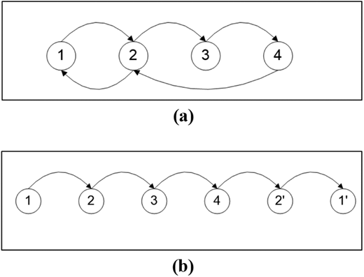
This study considers a typical liner shipping route, which includes I = {1,…, n} ports of call. The port rotation (i.e. sequence of visited ports) is assumed to be known, as this decision is usually made by the liner shipping company at the strategic level (Meng et al., 2014). Each port of call is visited once; however, the proposed methodology can be also used for liner shipping routes, where a given port of call is visited more than once. In the latter situation (i.e. when a given port of call is visited more than once), an additional node will be added to the graph, which represents the port rotation, to account for the second visit to the same port. For example, the liner shipping route, presented in Figure 1(a), includes a total of four ports. Ports 1 and 2 are visited twice; hence, two additional nodes 1′ and 2′ are introduced to the graph, and the total number of ports to be visited will be |I| = 4 + 2 = 6 [Figure 1(b)].
A vessel sails between two consequent ports i and i + 1 along leg i. It is assumed that certain legs of a liner shipping route pass through ECAs. The subset of voyage legs, passing through ECAs, will be referred to as I*, whereas the rest of voyage legs (passing outside ECAs) will belong to subset I0. Note that I0∪I* = I,I0∩I* = ∅. The liner shipping company should provide service with a certain frequency at each port of call (typically weekly or bi-weekly service). The terminal operator at each port establishes a specific arrival time window – TW [– start of TW at port i, – end of TW at port i], during which a vessel should arrive at the given port of call. Duration of a TW may vary from one to three days depending on the port (OOCL, 2016). The service of a vessel is assumed to start upon its arrival. If a vessel arrives at port i prior to the start of TW, it will be waiting for service at a dedicated area. A monetary penalty will be imposed on the liner shipping company if a vessel arrives after the end of TW (Dulebenets et al., 2015a). The container demand (measured in TEUs) at each port of call is assumed to be known (Meng et al., 2014).
3.1 Vessel service at ports
This study assumes that a liner shipping company has contractual agreements with marine container terminal operators. Based on those agreements, each marine container terminal operator is able to offer a set of handling rates Si = {1,…, hi}∀i∈I to the liner shipping company. Each handling rate has a corresponding handling productivity dis∀i ∈ I, s ∈ Si, measured in TEUs per hour. Vessel handling time pis∀i ∈ I, s ∈ Si (in hours) is estimated based on the container demand at a given port and the handling productivity requested. Note that a handling rate, which has a higher handling productivity, will reduce the vessel handling time at a given port of call but will increase the port handling cost for the liner shipping company.
3.2 Bunker consumption
The vessel fleet, serving a given liner shipping route, is assumed to be homogeneous (i.e. all vessels in the fleet have the same/similar technical characteristics). The latter practice has been widely adopted in the vessel scheduling literature (Wang and Meng, 2012a, 2012b, 2012c; Wang et al., 2013, 2014). The bunker consumption is assumed to be proportional to the vessel sailing speed and can be computed from the following equation (Du et al., 2011; Wang and Meng, 2012b):
Where:
- q(v̄)
= daily bunker consumption by vessel (tons of fuel/day);
- v̄
= average daily vessel sailing speed (knots);
- q(v*)
= daily bunker consumption by vessel when sailing at the designed speed (tons of fuel/day);
- v*
= design vessel sailing speed (knots); and
- α,γ
= bunker consumption coefficients.
Technically, to determine the values of bunker consumption coefficients α and γ, the regression analysis should be performed for each vessel in the fleet (Du et al., 2011; Wang and Meng, 2012b). This study will use the most common values of the bunker consumption coefficients revealed in the literature (Psaraftis and Kontovas, 2013; Wang and Meng, 2012b): α = 3 and γ = 0.012. Once the liner shipping company makes a decision on a vessel sailing speed between consequent ports of call, it will remain constant. The factors that may influence the vessel speed throughout the voyage (e.g. weather, height of waves, speed of wind, etc.) are not modeled. The bunker consumption by auxiliary engines will be included as a part of the weekly vessel operational cost. The bunker consumption f(vi) can be computed per nautical mile at leg i using the following equation:
Where:
- li
= length of voyage leg i, which connects ports i and i + 1 (nmi); and
- ti
= sailing time between ports i and i + 1 (hours).
3.3 Inventory cost
In the design of the vessel schedule, the liner shipping company has to consider the inventory cost, which is proportional to the total transit time. The total inventory cost of containers, which are transported at the given liner shipping route, can be estimated using the following equation (Wang et al., 2014):
Where:
- IC
= total inventory cost (USD);
- μ
= unit inventory cost (USD per TEU per hour); and
- NCTi
= quantity of containers transported at leg i (TEUs).
3.4 Existing International Maritime Organization regulations
The existing IMO regulation requires that the sulfur content in the fuel cannot exceed 0.1 per cent when passing through SOx ECAs (IMO, 2016a). This study assumes that the vessels use Marine Gas Oil (MGO) with sulfur content Pi = 0.1%∀i ∈ I* at voyage legs passing through ECAs. At the rest of voyage legs, the vessels use Heavy Fuel Oil (HFO) with sulfur content Pi = 3.5%∀i ∈ I0. Furthermore, the diesel engines of vessels, deployed at the given liner shipping route, comply with Tier III limits in case of ECAs with restrictions on NOx emissions. The latter assumption can be relaxed for liner shipping routes passing though ECAs with SOx control only (e.g. Baltic Sea and North Sea).
3.5 Emission restrictions
The scope of this study includes modeling of the environmental policy, which not only complies with the existing IMO regulations but also enforces restrictions on the actual quantity of emissions produced within ECAs. NOx emissions are regulated by enforcing requirements on diesel engines. Hence, given configuration of a diesel engine and its maximum operating speed, the vessel will not be able produce more NOx emissions than established by the IMO limit. As for sulfur emissions (i.e. SOx, sulfur dioxide [SO2] and particulate matter), they are regulated by enforcing restrictions on the type of fuel within ECAs. Use of low sulfur fuel will reduce the quantity of sulfur emissions, but the total quantity still can be substantial when vessels are sailing at high speeds through ECAs. As SO2 emissions comprise 98 per cent of sulfur emissions (Kontovas 2014), this study will model restrictions on SO2 emissions only.
3.6 Emission estimation
The quantity of SO2 emissions is significantly affected with the quantity of sulfur in the fuel. SO2 emissions (in tons) at leg i can be computed based on the percentage of sulfur in the fuel (Pi∀i ∈ I, per cent) and factor 0.02, which indicates that only 2 per cent of sulfur will react with oxygen and produce SO2 emissions (Kontovas 2014):
3.7 Decisions
The problem studied herein can be categorized as a tactical-level problem and will be referred to as the green vessel scheduling problem in a liner shipping route with ECAs. The liner shipping company has to determine the following in this problem:
the quantity of vessels required to provide the agreed service frequency at each port of the port rotation (assumed to be one week);
the vessel sailing speed between consequent ports of call;
one of the available handling rates at each port;
the waiting time at each port, belonging to the liner shipping route; and
the hours of vessel late arrival at each port of call.
The above mentioned decisions that have to be made by the liner shipping company in this problem are interrelated. Before deciding on a vessel sailing speed at a given voyage leg, the liner shipping company should consider the limits on vessel sailing speed (vmin ≤ vi ≤ vmax∀i ∈ I), bunker consumption, inventory costs, vessel emissions and emission restrictions within ECAs. The liner shipping company may use the concept of slow steaming to reduce bunker consumption and associated emissions. The latter will increase the total transit time of containers and will require deployment of more vessels to ensure that the weekly service is provided at each port of the port rotation. In the meantime, the liner shipping company must account for the limit on quantity of vessels (q ≤ qmax) allocated for service of the given liner shipping route. Availability of multiple handling rates at ports of call allows the liner shipping company to consider different alternatives between sailing and port handling times (e.g. selection of a handling rate with a higher productivity will decrease the handling time at a given port of call and will allow sailing at a lower speed to the next port of the port rotation).
4. Mathematical models
This section presents two mathematical models: the green vessel scheduling problem, which enforces the existing IMO regulations and ensures that a low- sulfur fuel is used at voyage legs passing through ECAs (will be referred to as GVSP1), and the green vessel scheduling problem, which imposes the requirements not only on the fuel type within ECAs but also on the quantity of emissions produced (will be referred to as GVSP2).
4.1 Nomenclature
4.1.1 Sets
4.1.2 Decision variables
4.1.3 Auxiliary variables
- q
= quantity of vessels assigned to the given liner shipping route (vessels)
= arrival time at port i (hours)
= departure time from port i (hours)
- wti∀i ∈ I
= waiting time of a vessel at port i (hours)
- ti∀i ∈ I
= sailing time of a vessel at voyage leg i (hours)
- f(vi)∀i ∈ I
= total bunker consumption by a vessel at voyage leg i (tons of fuel/nmi)
- lti∀i ∈ I
= vessel late arrival at port i (hours)
4.1.4 Parameters
- βi∀i ∈ I
= unit bunker cost when sailing at voyage leg i (USD/ton)
- cOC
= vessel weekly operational cost (USD/week)
= delayed arrival penalty at port i (USD/h)
- μ
= unit inventory cost (USD per TEU per h)
- li∀i ∈ I
= length of voyage leg i (nmi)
- NCTi∀i ∈ I
= quantity of containers transported at voyage leg i (TEUs)
- vmin
= minimum sailing speed of a vessel (knots)
- vmax
= maximum sailing speed of a vessel (knots)
- qmax
= maximum quantity of vessels that can be assigned for service of the given liner shipping route (vessels)
= start of TW at port i (hours)
= end of TW at port i (hours)
- tcis∀i ∈ I, s ∈ Si
= handling cost of a vessel at port i under handling rate s (USD)
- pis∀i ∈ I, s ∈ Si
= handling time of a vessel at port i under handling rate s (hours)
4.2 The green vessel scheduling problem with the existing International Maritime Organization regulations
The mixed-integer non-linear green vessel scheduling problem GVSP1 can be formulated as follows:
GVSP1
subject to:
and
In GVSP1, the liner shipping company aims to minimize the total route service cost (5), which consists of five components:
total vessel weekly operational cost;
total bunker consumption cost;
total port handling cost;
total late arrival penalty; and
total inventory cost.
Note that the unit bunker cost βi varies at voyage legs. A more expensive low- sulfur MGO is used at voyage legs passing through ECAs (βi = βMGO ∀ i ∈ I*, where βMGO – the unit MGO cost), whereas HFO is used at the rest of the voyage legs (βi = βHFO ∀ i ∈ I0, where βHFO – the unit HFO cost). Constraints set (6) ensures that only one handling rate should be selected by the liner shipping company at each port of the port rotation. Constraints set (7) estimates a sailing time of vessel between consequent ports i and i + 1. Constraints set (8) indicates that a vessel cannot be served at port i before the start of TW. Constraints sets (9) and (10) calculate waiting time of a vessel at port i. Constraints set (11) computes departure time of a vessel from port i. Constraints set (12) calculates late arrival hours of a vessel at port i. Constraints sets (13) and (14) estimate arrival time of a vessel at the next port of the port rotation. Constraints set (15) indicates that the weekly service at each port of call should be met (168 represents the total number of hours in a week). The right-hand-side of the inequality calculates the total turnaround time of a vessel at the given liner shipping route and includes three components:
the total sailing time;
the total port handling time; and
the total port waiting time.
Constraints set (16) indicates that the quantity of vessels assigned for service of the given liner shipping route cannot exceed the quantity of available vessels. Constraints set (17) establishes bounds on sailing speed of a vessel at voyage leg i. Constraints (18)-(20) define ranges of variables and parameters.
4.3 The green vessel scheduling problem with emission restrictions
Denote RSO2 as the restriction on production of SO2 emissions (tons) at voyage leg i. Then, the mixed-integer non-linear green vessel scheduling problem GVSP2 that accounts for the requirements not only on the fuel type within ECAs but also on the quantity of SO2 emissions produced can be formulated as follows:
GVSP2
subject to:
Constraint sets (6)-(20).
and
5. Solution approach
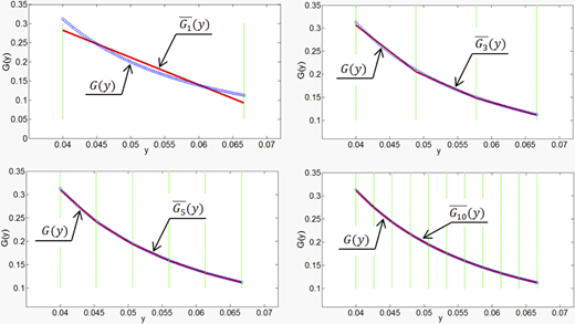
GVSP1 is a non-linear mathematical model due to: 1) objective function (5); and 2) constraints set (7). Non-linearity of GVSP2stems from: 1) objective function (21); and 2) constraints sets (7) and (22). This section discusses how both models can be reformulated as liner problems. Replacing of vessel sailing speed vi with its reciprocal yi = 1/vi will linearize constraints set (7). Denote G(y) as the bunker consumption function estimated based on vessel sailing speed reciprocal y. The non-linear bunker consumption function G(y) can be linearized using its piecewise linear secant approximation Gm(y), where m is the quantity of linear segments in the piecewise function (Wang et al., 2013). Figure 2 shows a few instances of piecewise linear secant approximations with various quantities of linear segments (m = 1,3,5,10) for the non-linear bunker consumption function G(y) = 0.012(y)−2/24. Lower and upper bounds on vessel sailing speed were set to vmin = 15 knots to vmax = 25 knots, respectively (i.e. 0.040 ≤ y ≤ 0.067). It can be observed that increasing quantity of linear segments m enhances the accuracy of approximation for G(y).
Let K = {1, 2,….m} be the set of linear segments in the piecewise function Gm(y). Let bik = 1 if linear segment k is chosen to approximate the bunker consumption function at voyage leg i (0 otherwise). Denote stk,edk,k ∈ K as the speed reciprocal values at the start and the end (respectively) of linear segment k; SLk,INk,k ∈ K as the slope and the intercept of linear segment k; and M1,M2 as sufficiently large positive numbers. Then, GVSP1 and GVSP2 can be reformulated as linear problems (that will be referred to as GVSPL1 and GVSPL2, respectively) as follows:
GVSPL1
subject to:
and
Constraints set (25) indicates that only one linear segment k will be chosen to approximate the bunker consumption function at voyage leg i. Constraints sets (26) and (27) define the range of values for the vessel sailing speed reciprocal, when linear segment k is chosen to approximate the bunker consumption function at voyage leg i. Constraints set (28) calculates the approximated bunker consumption value at voyage leg i. Constraints set (29) estimates the sailing time of a vessel between consequent ports i and i + 1. Constraints set (30) establishes bounds on sailing speed of a vessel at voyage leg i. Strict lower bounds for M1 and M2 can be defined as follows: M1 = 1/vmin, M2 = SL1 (1/vmax) + IN1. Note that parameters M1 and M2 in constraints sets (27) and (28) can be substituted with M = max{M1; M2}.
GVSPL2
subject to:
In GVSPL2, objective function (31) aims to minimize the total route service cost. Constraints set (32) calculates SO2 emissions at voyage leg i.
There are two types of the secant approximations (Wang et al., 2013):
the static secant approximation, SSA; and
the dynamic secant approximation, DSA.
If SSA is used, the quantity of linear segments in the approximation is fixed, and GVSPL1 and GVSPL2 should be solved only once. If DSA is used, the quantity of linear segments in the approximation is a variable, and GVSPL1 and GVSPL2 should be solved iteratively by increasing the quantity of segments until the desired solution accuracy is achieved. The advantage of SSA is that GVSPL1 and GVSPL2 should be solved only once; however, if a large quantity of segments is used, the computational time may be significant. This study will use DSA to solve GVSPL1 and GVSPL2. The main DSA steps are outlined in Procedure 1 for GVSPL1. Note that similar steps were performed to solve GVSPL2. In Step 1, the initial quantity of segments in the approximation is set to m = 0 and the initial accuracy is set to Δ = 100. Note that the initial accuracy can be set to any number greater than the target accuracy (i.e. Δ > Δt). Then, DSA enters the loop, where in Step 3, one segment is added to the approximation. Then, in Step 4, GVSPL1 with the updated quantity of segments is solved, and a new vessel schedule VS and the associated objective function value Z are obtained. In Step 5, function EstObj(InputData, VS) estimates the true value of the objective function Z* (i.e. value of the non-linear objective function at the solution VS, provided by GVSPL1). In Step 6, the solution accuracy is updated. DSA terminates when the target accuracy of GVSPL1 solution is achieved. Performance of DSA will be evaluated against SSA in the numerical experiments section.
Procedure 1. Dynamic Secant Approximation (DSA)
DSA(InputData, Δt)
in: InputData – liner shipping route characteristics; Δt – target accuracy
out: VS – vessel schedule
1: m ← 0, Δ ← 100 ◁ Initialization
2: while Δ > Δt do
3: m ← m + 1 ◁ Increase the quantity of segments in the approximation
4: [Z, VS] ← GVSPL1 (InputData, m) ◁ Solve GVSPL1 with m segments
5: Z* ← EstObj (InputData, VS) ◁ Estimate the non-linear objective function value
6: Δ ← |Z* − Z|/Z* ◁ Update the accuracy
7: end while
8: return VS
6. Numerical experiments
This section presents numerical experiments that were undertaken to evaluate the performance of the proposed solution approach and assess advantages and disadvantages from enforcing emission restrictions within ECAs.
6.1 Input data description
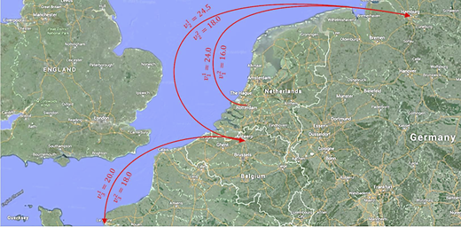
This study considers the French Asia Line 3 route (Figure 3), which is served by CMA CGM (2016) liner shipping company. This liner shipping route connects North Europe, Red Sea and Asia. The port rotation for the French Asia Line 3 route includes 13 ports of call (the distances between consequent ports in nautical miles are shown in parenthesis and were retrieved from the world seaports catalogue [1]), where the Port of Kelang (Malaysia) and Port of Le Havre (France) are visited twice:
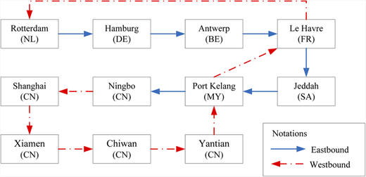
1. Rotterdam, NL (341) → 2. Hamburg, DE (426) → 3. Antwerp, BE (244) → 4. Le Havre, FR (4,403) → 5. Jeddah, SA (4,455) → 6. Port Kelang, MY (2,835) → 7. Ningbo, CN (87) → 8. Shanghai, CN (606) → 9. Xiamen, CN (731) → 10. Chiwan, CN (395) → 11. Yantian, CN (2,045) → 12. Port Kelang, MY (8,857) → 13. Le Havre, FR (355) → 1. Rotterdam, NL.
The available liner shipping literature (Wang and Meng, 2012a, 2012b, 2012c; Zampelli et al., 2014; OOCL, 2016; World Shipping Council, 2016, etc.) was used to generate the numerical data necessary for computational experiments (Table I). The end of TW at each port of the port rotation was estimated using the end of TW at preceding port, length of a voyage leg between consequent ports and bounds of the vessel sailing speed: , where U is a notation for uniformly distributed pseudorandom numbers. The quantity of containers, transported at voyage leg iwas generated as NCTi = U[5,000; 8,000]∀i ∈ I TEUs.
Numerical data
| Parameter | Value | Source(s) |
|---|---|---|
| Bunker consumption coefficients: α,γ | α = 3, γ = 0.012 | Du et al. (2011), Wang and Meng (2012b), Psaraftis and Kontovas (2013) |
| Unit HFO cost: βHFO (USD/ton) | 300 | Fagerholt and Psaraftis (2015) |
| Unit MGO cost: βMGO (USD/ton) | 600 | Fagerholt and Psaraftis (2015) |
| Weekly operational cost of a vessel: cOC (USD/week) | 300,000 | Wang and Meng (2012a, 2012b, 2012c) Dulebenets (2015, 2016), |
| Delayed arrival penalty: (USD/hours) | U [5,000; 10,000] | Zampelli et al. (2014) |
| Unit inventory cost: μ (USD per TEU per hour) | 1 | Wang et al. (2014), Dulebenets et al. (2015a) |
| Percent of sulphur in MGO: PMGO (%) | 0.1 | Psaraftis and Kontovas (2013), Kontovas (2014) |
| Percent of sulphur in HFO: PHFO (%) | 3.5 | Psaraftis and Kontovas (2013), Kontovas (2014) |
| Duration of TW (hours) | U [24; 72] | OOCL (2016) |
| Minimum sailing speed of a vessel: vmin (knots) | 15 | Wang and Meng (2012a, 2012b, 2012c) |
| Maximum sailing speed of a vessel: vmax (knots) | 25 | Wang and Meng (2012a, 2012b, 2012c) |
| Maximum quantity of deployed vessels: qmax | 15 | Wang and Meng (2012a, 2012b, 2012c) |
The weekly container demand NCi at large ports of the port rotation was assigned as U[500;2,000] TEUs. Note that a given port was considered as a “large port” only if it belonged to the list of top 20 world container ports based on the overall throughput (World Shipping Council, 2016). The weekly container demand at smaller ports was generated as U[200;1,000] TEUs. This study assumes that the following handling productivities (dis) were offered to the liner shipping company at large ports: [125; 100; 75; 50] TEUs/h. At smaller ports, the liner shipping company was able to request [100; 75; 60; 50] TEUs/h or [75; 70; 60; 50] TEUs/h. The assumption regarding the handling productivities can be justified by the fact that marine container terminal operators at large ports typically have more equipment available for serving vessels and, hence, are able to provide more handling rate alternatives to the liner shipping company. In the meantime, increasing quantity of TEUs handled may increase productivity.
Based on the established IMO regulations, the North Sea and the English Channel were designated as SOx ECAs for the considered liner shipping route (IMO, 2016a). The restrictions on quantity of SO2 emissions produced at voyage legs passing through ECAs were assigned as follows: RSO2i = 0.02Piγli(U[vmin; vmax])a−1/24∀i∈I* tons. The vessel handling cost per TEU scis at port i under handling rate s was estimated as: scis = mhc±U[0; 50]∀i∈I, s∈Si USD/TEU, where mhc is the mean handling cost. Then, the overall port handling cost was computed as: tcis = scisNCi∀i∈I,s∈Si USD. The mhc was set equal to [700; 625; 550; 475] USD/TEU for four available handling rates, respectively (World Bank, 2016; The Port Authority of New York and New Jersey, 2016; Dulebenets et al., 2015b). This study also assumes that each marine container terminal operator perceives the vessel handling cost differently (i.e. vessel handling charge for the same handling rate varies from one port to the other). The latter aspect is captured for by the second (and random) term of the scis equation.
All numerical experiments were conducted on a Dell T1500 Intel(T) Core i5 Processor with 2.00 GB RAM. MATLAB (2014a) was used to develop the secant approximations for the bunker consumption function (Mathworks, 2016). GVSPL1 and GVSPL2 were solved using CPLEX of General Algebraic Modeling System at each iteration of DSA.
6.2 Performance of the solution approach
DSA was compared against SSA with m = 100 segments. A total of 20 instances were developed using the data, described in Section 6.1 and presented in Table I, by changing the service TWs at ports and TW duration. The target accuracy for DSA was set to Δt = 0.1%. GVSPL1 and GVSPL2 were solved using SSA and DSA for each one of the generated instances, and results are presented in Table II, including the following information for SSA and DSA:
instance number;
quantity of linear segments (m) used in the approximation to solve the problem;
objective gap Δ = |(Z* − Z)/Z*|, where Z is GVSPL1/GVSPL2 objective function value and Z* is value of the non-linear objective function at the solution, provided by GVSPL1/GVSPL2; and
average over five replications of CPU time.
Performance of the solution approach
| Instance | Quantity of segments GVSPL1/GVSPL2 | Objective gap GVSPL1/GVSPL2 | CPU Time, s GVSPL1/GVSPL2 | |||
|---|---|---|---|---|---|---|
| SSA | DSA | SSA | DSA | SSA | DSA | |
| I1 | 100/100 | 5/5 | 2.0E−14/7.9E−08 | 9.6E−04/5.6E−04 | 20.4/12.2 | 0.9/0.9 |
| I2 | 100/100 | 5/5 | 1.9E−14/7.2E−08 | 9.0E−04/5.3E−04 | 18.2/11.7 | 0.9/0.9 |
| I3 | 100/100 | 5/4 | 2.0E−14/8.0E−08 | 9.4E−04/9.7E−04 | 20.6/12.4 | 0.9/0.6 |
| I4 | 100/100 | 5/4 | 1.9E−14/7.5E−08 | 8.9E−04/9.5E−04 | 20.1/11.6 | 1.0/0.6 |
| I5 | 100/100 | 5/5 | 2.0E−14/7.4E−08 | 9.3E−04/5.9E−04 | 17.4/12.4 | 0.9/0.9 |
| I6 | 100/100 | 5/5 | 1.9E−14/7.7E−08 | 8.7E−04/4.8E−04 | 20.3/12.3 | 0.9/0.9 |
| I7 | 100/100 | 5/4 | 2.0E−14/7.8E−08 | 9.2E−04/9.9E−04 | 20.5/12.4 | 0.9/0.6 |
| I8 | 100/100 | 5/5 | 2.0E−14/7.7E−08 | 9.1E−04/6.9E−04 | 20.4/12.3 | 0.9/0.9 |
| I9 | 100/100 | 5/5 | 2.0E−14/8.1E−08 | 9.0E−04/6.8E−04 | 20.4/12.3 | 0.9/0.9 |
| I10 | 100/100 | 5/4 | 2.0E−14/8.0E−08 | 8.5E−04/9.6E−04 | 20.7/12.4 | 0.9/0.6 |
| I11 | 100/100 | 5/5 | 1.9E−14/7.0E−08 | 8.9E−04/5.7E−04 | 17.6/11.8 | 0.9/0.9 |
| I12 | 100/100 | 5/5 | 1.9E−14/7.5E−08 | 9.3E−04/6.0E−04 | 17.9/12.2 | 0.9/0.9 |
| I13 | 100/100 | 5/4 | 2.0E−14/8.1E−08 | 9.1E−04/9.4E−04 | 20.6/12.4 | 0.9/0.6 |
| I14 | 100/100 | 5/5 | 2.0E−14/8.1E−08 | 9.3E−04/5.9E−04 | 20.5/12.4 | 0.9/0.9 |
| I15 | 100/100 | 5/5 | 2.0E−14/7.8E−08 | 8.9E−04/4.8E−04 | 20.4/12.3 | 0.9/0.9 |
| I16 | 100/100 | 5/5 | 2.0E−14/8.1E−08 | 9.2E−04/5.4E−04 | 20.4/12.4 | 0.9/0.9 |
| I17 | 100/100 | 5/4 | 2.0E−14/8.1E−08 | 8.6E−04/9.4E−04 | 20.5/12.4 | 0.9/0.6 |
| I18 | 100/100 | 5/5 | 1.9E−14/7.1E−08 | 9.0E−04/5.8E−04 | 18.3/11.4 | 0.9/0.9 |
| I19 | 100/100 | 5/4 | 2.0E−14/8.1E−08 | 9.4E−04/9.1E−04 | 20.6/12.4 | 0.9/0.5 |
| I20 | 100/100 | 5/4 | 2.0E−14/7.8E−08 | 9.1E−04/9.4E−04 | 20.5/12.3 | 0.9/0.6 |
| Average: | 100/100 | 5.0/4.6 | 2.0E−14/7.7E−08 | 9.1E−04/7.2E−04 | 19.8/12.2 | 0.9/0.8 |
For example, SSA required 100 linear segments to solve GVSPL1 for problem instance I3 with the objective gap of 2.0E−14 and computational time of 20.6 s. For the same problem instance (I3), DSA required five linear segments to solve GVSPL1 with the objective gap of 9.4E−04 and computational time of 0.9 s.
It can be observed that on average, over the considered problem instances, DSA required five linear segments in the approximation to solve GVSPL1 and GVSPL2 with the target accuracy, which is significantly smaller as compared to the quantity of segments in SSA. Objective gaps, produced by DSA, were larger as compared to the ones produced by SSA. The latter can be explained by the fact that SSA used much more segments for the bunker consumption function approximation. The average over five replications and 20 problem instances of DSA CPU time comprised 0.9 and 0.8 s for GVSPL1 and GVSPL2, respectively. The average over five replications and 20 problem instances of SSA CPU time comprised 19.8 and 12.2 s for GVSPL1 and GVSPL2, respectively. Results from the computational experiments demonstrate that DSA was able to achieve the target accuracy within significantly smaller CPU time as compared to SSA for all generated problem instances, which indicates the efficiency of the proposed solution approach.
6.3 Managerial insights
The total route service cost and its components were estimated after obtaining the solutions for GVSPL1 and GVSPL2 for each one of the considered problem instances. Results are presented in Figure 4, including the following cost components: the total route service cost, Z; the total weekly vessel operational cost, OC; the total bunker consumption cost, BC; the total port handling cost, PC; the total late arrival penalty, LP; and the total inventory cost, IC.
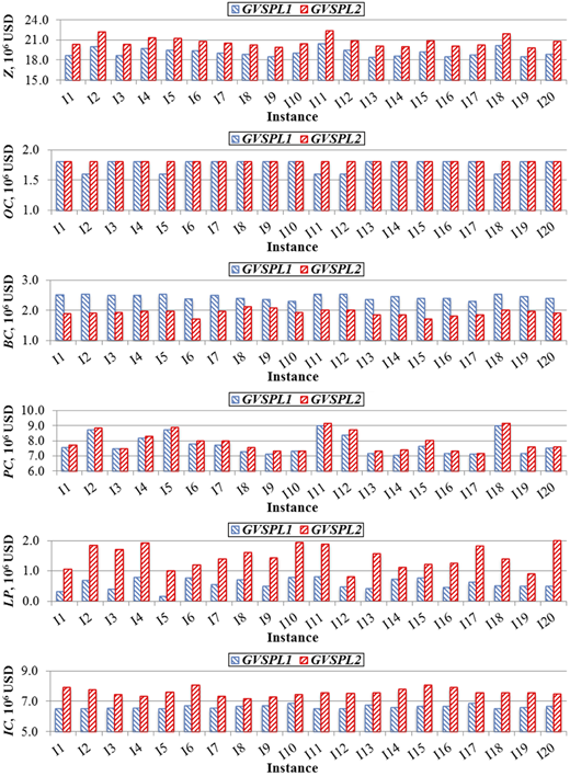
We observe that all route service cost components, except the bunker consumption cost, are greater (or equal in some instances) for GVSPL2 vessel schedules, as compared to GVSPL1 vessel schedules. The restrictions on the quantity of emissions produced within ECAs decrease the bunker consumption cost (i.e. the vessel sailing speed is reduced to comply with the emission restrictions at voyage legs passing through ECAs) for vessel schedules provided by GVSPL2. Moreover, port handling costs are higher for GVSPL2 vessel schedules as compared to GVSPL1 vessel schedules. The latter can be explained by the fact that introduction of emission restrictions would require the liner shipping company to select handling rates with a higher productivity to save time in ports. Savings in port times can be further used by the liner shipping company to increase the vessel sailing time within ECAs (i.e. sail at a lower speed to the consequent port of the port rotation and reduce the quantity of emissions produced within ECAs).
GVSPL2 produces vessel schedules with the late arrival penalty, which is substantially higher as compared to the late arrival penalty associated with GVSPL1 vessel schedules. Increase in the late arrival penalty for GVSPL2 vessel schedules indicates that the liner shipping company may have to violate the port arrival TWs, negotiated with marine container terminal operators, to meet the restrictions on the quantity of emissions produced within ECAs. Because of increasing vessel sailing time, the total inventory cost is higher for vessel schedules, suggested by GVSPL2, as compared to GVSPL1 vessel schedules. Furthermore, GVSPL2 vessel schedules have higher vessel weekly operational cost for certain instances (i.e. I2, I5, I11, etc.). The latter can be explained by the fact that increase in sailing time for GVSPL2 schedules requires deployment of more vessels at the given liner shipping route to guarantee the weekly service at each port of the port rotation. It was found that on average, over all considered problem instances, the total route service cost could increase by 7.8 per cent from introducing restrictions on the quantity of SO2 emissions produced within ECAs. A detailed comparison of GVSPL1 and GVSPL2 vessel schedules in terms of sailing speed selection within ECAs, bunker consumption, emissions produced within ECAs and port late arrivals is presented next.
6.3.1 Vessel sailing speed selection within Emission Control Areas.
The vessel sailing speeds were retrieved for GVSPL1 and GVSPL2 schedules for each one of the considered problem instances at three voyage legs passing through ECAs:
voyage leg 1: Rotterdam (NL) to Hamburg (DE);
voyage leg 2: Hamburg (DE) to Antwerp (BE); and
voyage leg 3: Antwerp (BE) to Le Havre (FR).
The average vessel sailing speeds (in knots) over the generated problem instances at voyage legs 1-3 are presented in Figure 5 for GVSPL1 and GVSPL2 vessel schedules. Notation was adopted for the vessel sailing speed at voyage leg i suggested by GVSPL1, whereas notation was adopted for the vessel sailing speed at voyage leg isuggested by GVSPL2. We observe that on average, the vessel sailing speed was reduced by 33.3, 26.5 and 10.0 per cent at voyage legs 1-3, passing through ECAs, when emission restrictions were imposed. Reduction in the vessel sailing speed increases the container transit time through ECAs but decreases the quantity of SO2 emissions produced.
6.3.2 Bunker consumption comparison.
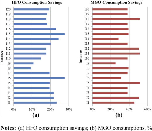
Vessel schedules, produced by GVSPL1 and GVSPL2, were compared in terms of the amount of fuel (both HFO and MGO) consumed by vessels serving the French Asia Line 3 route. As GVSPL2 vessel schedules have lower bunker consumption costs (Section 6.3 and Figure 4) as compared to GVSPL1 vessel schedules, the total bunker consumption was also found to be lower for all the considered problem instances. Furthermore, numerical experiments demonstrate that GVSPL2 vessel schedules not only required less MGO at voyage legs, passing through ECAs, but also yielded HFO savings. The bunker consumption savings were estimated for all generated problem instances, and results are presented in Figure 6 for HFO and MGO fuel types. We observe that on average, GVSPL2 vessel schedules require 19.6 per cent less HFO and 40.4 per cent less MGO. The MGO savings can be explained by the fact that the liner shipping company was required to decrease the vessel sailing speed (hence, reduce the MGO consumption) at voyage legs, passing through ECAs, to avoid violation of the emission restrictions. In the meantime, introduction of emission restrictions reduced vessel sailing speeds not only within ECAs but also at the adjacent voyage legs, which yielded the HFO consumption savings.
6.3.3 Emission comparison.
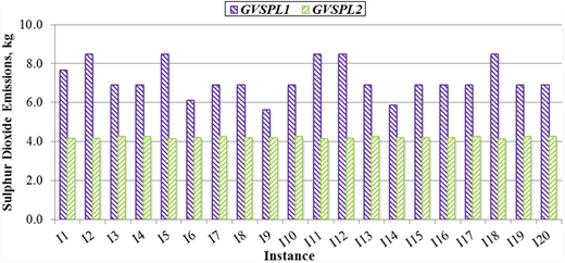
The total quantity of SO2 emissions was calculated for GVSPL1 and GVSPL2 vessel schedules at voyage legs within ECAs for all the considered problem instances, and results are presented in Figure 7. Numerical experiments showcase that introduction of emission restrictions at voyage legs, passing through ECAs, in GVSPL2 vessel schedules reduced the quantity of SO2 emissions by 40.4 per cent (i.e. proportional to the MGO consumption savings). We observe that on average, GVSPL1 vessel schedules produced 7.2 kg of SO2, whereas GVSPL2 vessel schedules produced 4.2 kg of SO2. Hence, enforcing emission restrictions within ECAs can significantly reduce the pollution levels.
6.3.4 Port late arrivals.
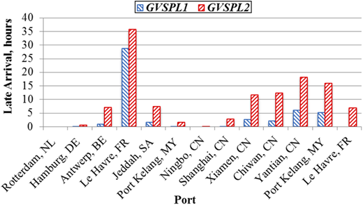
The hours of late arrivals at ports of call were estimated for GVSPL1 and GVSPL2 vessel schedules for all 20 problem instances, and the average values are shown in Figure 8 for each port of call. As GVSPL2 vessel schedules have higher late arrival penalties (Section 6.3 and Figure 4) as compared to GVSPL1 vessel schedules, the hours of late vessel arrivals to ports of call were also found to be higher for all the considered problem instances. The increase in hours of late arrivals for GVSPL2 vessel schedules as compared to GVSPL1 vessel schedules was recorded not only at ports located within ECAs (i.e. Rotterdam, NL; Hamburg, DE; Antwerp, BE; and Le Havre, FR) but also at ports located outside ECAs (e.g. Yantian, CN; Port Kelang, MY; etc.). Hence, introduction of emission restrictions required the liner shipping company to make significant changes in the vessel schedule. Results from computational experiments indicate that the hours of port late arrivals may increase on average by 152.8 per cent from imposing the emission restrictions within ECAs.
6.4 Discussion
This study proposes two mathematical models for the green vessel scheduling problem in a liner shipping route with ECAs. The first mathematical model captures the existing IMO regulations, whereas the second one complies not only with the established IMO requirements within ECAs but also enforces restrictions on the actual quantity of emissions produced. Numerical experiments, performed for the French Asia Line 3 route, demonstrate that introduction of emission restrictions on average reduces the quantity of emissions produced by 40.4 per cent. Furthermore, emission restrictions will require the liner shipping company to decrease vessel sailing speeds within ECAs, which shall result in bunker consumption savings but an increase in the transit time of containers and, in turn, an increase in the total inventory cost. Increase in the transit time of containers (hence, increase in the total vessel turnaround time) may require deployment of more vessels to ensure the weekly service frequency at ports of call. It was found that the total vessel route service cost might increase by 7.8 per cent from imposing restrictions on the emissions produced within ECAs.
In conclusion, advantages from enforcing emission restrictions within ECAs can be summarized as follows:
reduction in the quantity of emissions produced;
improving the environmental sustainability;
reduction in the bunker consumption (both MGO and HFO fuel types); and
reduction in the total bunker consumption cost.
The list of disadvantages from enforcing emission restrictions within ECAs includes the following:
increase in the total weekly vessel operational cost;
increase in the total port handling cost;
potential late vessel arrivals to ports of call;
increase in the total transit time of containers and associated inventory costs; and
increase in the total route service cost.
7. Conclusions and future research
Considering a rapidly growing attention of the community to the environmental concerns, liner shipping companies should implement new strategies for developing their vessel schedules and improving environmental sustainability. The existing environmental regulations in liner shipping do not enforce any restrictions on the actual quantity of emissions that could be produced within ECAs. This study performed a comprehensive assessment of advantages and disadvantages from enforcing emission restrictions within ECAs. Two mixed-integer non-linear mathematical models were developed to achieve the latter objective. The first program modeled the existing IMO regulations, whereas the second one along with the established IMO requirements also enforced restrictions on the quantity of emissions produced within the ECAs. The objective of both models was to minimize the total route service cost. The original models were linearized and solved using the dynamic secant approximation procedure. Numerical experiments were conducted for the French Asia Line 3 route, served by CMA CGM liner shipping company and passing through ECAs with SOx control.
Results demonstrated that the proposed solution approach outperformed the static secant approximation procedure and was able to achieve the target accuracy within a significantly smaller computational time. Furthermore, introduction of emission restrictions reduced the quantity of SO2 emissions produced by 40.4 per cent. In the meantime, emission restrictions required the liner shipping company to decrease the vessel sailing speed not only at voyage legs within ECAs but also at the adjacent voyage legs, which increased the total vessel turnaround time and in turn increased the total route service cost by 7.8 per cent. The developed mathematical model can serve as an efficient practical tool for liner shipping companies in developing green vessel schedules, enhancing energy efficiency and improving environmental sustainability. The future research may consider the following extensions:
implement the developed mathematical models for various liner shipping routes;
consider heterogeneous vessel fleet (i.e. vessels, serving a given liner shipping route, have different technical characteristics);
account for uncertainty in bunker consumption; and
account for uncertainty in port handling times.
Note
Available at: www.searates.com
This work was partially supported by the Department of Civil Engineering at the University of Memphis (Memphis, TN) and the Department of Civil and Environmental Engineering at the Florida A&M University – Florida State University (Tallahassee, FL). Any opinions, findings, conclusions, or recommendations are those of the author and do not necessarily reflect the views of the aforementioned organizations.
