


A combined approach of additive Holt–Winters, support vector regression, simple moving average and generalized simulated annealing with error correction and optimal parameter selection techniques emphasizing optimal smoothing period in residual adjustment is developed and proposed to predict datasets of container throughput at major ports.
The additive Holt–Winters model describes level, trend and seasonal patterns to provide smoothing values and residuals. In addition, the fitted additive Holt–Winters predicts a future smoothing value. Afterwards, the residual series is improved by using a simple moving average with the optimal period to provide a more obvious and steady series of the residuals. Subsequently, support vector regression formulates a nonlinear complex function with more obvious and steady residuals based on optimal parameters to describe the remaining pattern and predict a future residual value. The generalized simulated annealing searches for the optimal parameters of the proposed model. Finally, the future smoothing value and the future residual value are aggregated to be the future value.
The proposed model is applied to forecast two datasets of major ports in Thailand. The empirical results revealed that the proposed model outperforms all other models based on three accuracy measures for the test datasets. In addition, the proposed model is still superior to all other models with three metrics for the overall datasets of test datasets and additional unseen datasets as well. Consequently, the proposed model can be a useful tool for supporting decision-making on port management at major ports in Thailand.
The proposed model emphasizes smoothing residuals adjustment with optimal moving period based on error correction and optimal parameter selection techniques that is developed and proposed to predict datasets of container throughput at major ports in Thailand.
1. Introduction
For international transportation, maritime transportation is a transportation mode for shipping by water to transfer and distribute cargo from origins to destinations and has been practiced for a long time. Moreover, maritime transportation plays an important role in international trade and the economies of many countries. In this regard, container throughput at major ports continuously increases over time, and there is more congested traffic at present. Consequently, the management of major ports is complex and challenging to increase competitive capability. Furthermore, investment and capital intensity are uncertain and risky in nature. Therefore, the major ports need to obtain useful information about the throughput of containers to operate and develop suitable strategies.
Thailand is a member of the Association of Southeast Asian Nations (ASEAN) and is a significant base of manufacturing and agricultural industries in ASEAN. Consequently, maritime transportation plays a vital role in international trade, which is a key factor in economic growth in Thailand. In the past, Bangkok Port (BKK Port) was established on the east side of the Chao Phraya River as Thailand’s main international port for transferring and distributing cargo inland. However, the Bangkok port limits access to ships with 12,000 tons of deadweight or less. Moreover, the ship’s size is no longer than 172 meters. To increase competitive capacity, Laem Chabang Port (LCB Port) as a deep seaport, which was a major port in the world 2023 and also plays a major port of international maritime transportation at present, was built on the east coast of the Gulf of Thailand to reduce problems and support the expansion of shipping.
For the intention of improving investment, planning and operations regarding port management, accuracy and reliability of forecasting methods are needed to support critical decision-making on port management at major ports (Cuong et al., 2021, 2022; Martius et al., 2022; Eskafi et al., 2021; He and Wang, 2021; Tan et al., 2021; Chan et al., 2019; Du et al., 2019). One of the most popular statistical methods for prediction is time series analysis, which is formulated from previous observations that only consist of container throughput volumes. Consequently, time-series analysis is a conventional approach for analyzing time-series patterns of container throughput and also provides reliable and good forecasts to support decision-making and planning.
One of the most popular time series methods is the autoregressive integrated moving average (ARIMA) (Sultanbek et al., 2024), which has dominated linear problems of time series and is quite often used as a benchmark for comparing forecasting performance (Jin et al., 2023; Munim et al., 2023; Xiao et al., 2023; Cui et al., 2022; Huang et al., 2020, 2022; Huang et al., 2022). However, the ARIMA methods cannot describe seasonal patterns of time series. Therefore, the seasonal autoregressive integrated moving average (SARIMA) method is designed to handle the time series of linear and seasonal patterns as an extended form of the ARIMA method (Halyal et al., 2022). For that reason, the SARIMA methods have been widely applied to many fields of monthly container throughput in recent years (Munim et al., 2023; Koyuncu et al., 2021).
On the other hand, a family of exponential smoothing methods is also one of the most popular statistical methods (Krembsler et al., 2024; Kumar et al., 2024; Svetunkov et al., 2023; Petropoulos et al., 2022; Moiseev, 2021), which is formulated from weighted averages of past observations, with the weights decaying exponentially for older observations to provide robust forecasts and reduce noise problems. Therefore, exponential smoothing methods have been overwhelmingly employed in the industrial and business domains in recent years. One of the most widely used methods of exponential smoothing is the Holt–Winters method, which is built from three equations to describe patterns of level, trend and seasonality in time series. Thus, the Holt–Winters method has been successful in monthly container throughput forecasting in recent years (Koyuncu et al., 2021; Shankar et al., 2020; Pang and Gebka, 2017).
Although both SARIMA and Holt–Winters methods have been successful in many fields of science and industry, they are utilized within the limits of linear problems. Moreover, it is difficult to diagnose whether the time series is generated from linear or nonlinear problems. Therefore, both SARIMA and Holt–Winters methods may not be appropriate for applications in real-world problems, especially nonlinear and complex problems.
In recent years, supervised machine learning methods have been developed and proposed to deal with time-series problems of container throughput for both complex and linear problems (Wang et al., 2024). One of the popular supervised machine learning methods is support vector regression (SVR), which is an extended form of a support vector machine for regression problems as well as time-series problems (Gatera et al., 2023; Moscoso-López et al., 2021; Chan et al., 2019). However, the SVR model has to be built with appropriate parameters to perform well in prediction. Therefore, metaheuristics are utilized to search for the proper parameters of the SVR model to reduce the risk of using improper parameters (Omar et al., 2024). One of the new metaheuristics is generalized simulated annealing (GenSA), which is developed and introduced in the class of stochastic algorithms to search for the global optimal solutions in continuous spaces (Xiang et al., 2013). Even though the combined approach of support vector regression and generalized simulated annealing, namely SVR-GenSA, can achieve higher accuracy than the approach of support vector regression, its performance based only on the structure of support vector regression may not be suitable for many problems in real-world situations.
Although individual forecasting models perform well in prediction to support decision-making, it is difficult to achieve more accuracy for many applications in real-world scenarios in order to reduce the risk of uncertainty. Accordingly, many combined approaches have been developed and proposed to address these problems. One of the widespread hybridizations is the combined approach of error correction, which emphasizes explaining residuals from the fitted model in the first phase by using another model. A combined approach of SARIMA and support vector regression methods is a well-known hybridization, which is formulated based on linear and nonlinear assumptions to describe both linear and nonlinear components in time series to aggregate both linear and nonlinear values to be a forecast value and achieve more accuracy (Huang et al., 2022; Xu et al., 2019; Mo et al., 2018; Niu et al., 2018). Moreover, the GenSA can improve the performance of the combined approach of SARIMA and support vector regression methods by searching for the most proper parameters of the SVR model to explain the pattern of the residual series. Therefore, the combined approach of SARIMA, SVR and GenSA methods (SARIMA-SVR-GenSA) may obtain more accuracy than only the combined approach of SARIMA and support vector regression methods for many problems.
Nevertheless, the SARIMA model may not provide good results in the first phase of the combined approach for many situations that affect the fitted residual series and are difficult to achieve more accuracy. For that reason, a combined approach of Holt–Winters and support vector regression methods is developed as an alternative approach, which exploits exponential smoothing techniques of Holt–Winters to provide forecasts in the first phase and the fitted residuals with robustness and noise reduction. Consequently, the smoothing residuals may provide an obvious pattern, which can enhance the combined model to forecast the future residual value and obtain more accuracy as well (Sujjaviriyasup, 2024; Moscoso-López et al., 2021).
Moreover, the performance of the combined approach can be improved by decreasing the problem regarding inappropriate parameters of the SVR model to achieve more accuracy. In this regard, the generalized simulated annealing method is utilized to search for appropriate parameters of the SVR model in the combined approach. Even though the combined approach of Holt–Winters, SVR and GenSA methods achieves more accuracy in forecasts, the performance of the combined approach may be improved by the more smoothing residual series of the Holt–Winters method using smoothing residual adjustment on the residual series to obtain more accuracy. Consequently, a new combined approach emphasizing optimal periods in residual adjustment has been developed and proposed to obtain higher accuracy.
The motivation of the proposed model aims at utilizing the advantage of equal weights from a simple moving average based on the given optimal period, which is obtained from the GenSA, to provide a more obvious and steady series of residuals. Afterwards, the SVR model with proper parameters obtained from the GenSA formulates a complex function based on a more obvious and smoothing series of residuals and predicts a future residual value. Finally, the predicted smoothing value from the additive Holt–Winters model and the predicted residual value from the SVR model are aggregated to be the forecast value. Moreover, the proposed model can be reduced to a combined model of additive Holt–Winters, SVR and GenSA when the period of moving average is equal to one. Thus, the proposed model can be generally built as the combined model of the additive Holt–Winters, SVR and GenSA with an optimal period of moving average to achieve more accuracy.
Experiments are presented in this research. Firstly, two datasets of container throughput at major ports in Thailand are analyzed with descriptive statistics for preliminary analysis. Moreover, all forecasting models are evaluated by using cross-validation for time series based on three well-known accuracy measures in the literature (Hyndman and Koehler, 2006): mean absolute error (MAE), mean absolute percentage error (MAPE) and symmetric mean absolute percentage error (sMAPE). For the accuracy measures, three well-known metrics are both scale-dependent and scale-independent measures, which are used to support the superior performance of the proposed model compared to other forecasting models.
The sections of this manuscript are presented as follows: first, the methods of forecasting models are described. Afterwards, the evaluations of forecasting performance are illustrated based on the cross-validation and accuracy metrics. Moreover, preliminary investigations and comparisons of forecast performances are analyzed and discussed. Then, the results and discussion are demonstrated. Finally, the highlighted findings and conclusions of the proposed model are summarized and presented.
2. Methodologies
2.1 Seasonal autoregressive integrated moving average
The seasonal autoregressive integrated moving average is an extension of the autoregressive integrated moving average, which is designed to handle datasets with seasonal patterns and is widely utilized in time-series problems. The mathematical expression is described in Eq. (1).
The is the dataset of container throughput at time t. refers to the non-seasonal autoregressive part with order p; refers to the seasonal autoregressive part with order P. Moreover, the and stand for the non-seasonal and seasonal moving average parts with orders q and Q, respectively. In addition, and refer to the non-seasonal and seasonal difference operators, respectively. The denotes white noise at time t. B is the backshift operator and s refers to the number of seasonal periods. For the most fitted SARIMA model, the lowest Akaike information criterion for a small sample size is selected to establish and determine the SARIMA model (Hyndman et al., 2022; Hyndman and Khandakar, 2008).
2.2 Holt–Winters
The Holt–Winters method is an exponential smoothing method that extends from Holt’s method to describe seasonal patterns of time series and is widely applied in many fields of science. The Holt–Winters method consists of one forecast equation and three smoothing equations to explain the level, trend and seasonality in time series with corresponding smoothing parameters and , respectively. In addition, the Holt–Winters method comprises two approaches, which are the additive Holt–Winters (AHW) method and the multiplicative Holt–Winters (MHW) method. The mathematical formulations of both AHW and MHW methods are presented in Eqs (2)–(9).
The additive Holt–Winters method can be demonstrated as follows:
The multiplicative Holt–Winters method can be expressed as follows:
where denotes an estimate of the level of the time series at time t. The is an estimate of the trend of the time series at time t; refers to an estimate of the seasonal component at time t. The m is the period of seasonality; k refers to the integer part of The is the predicted value at time t + h with the given previous datasets. In order to optimize the fitted Holt–Winters model, the most proper model is built by selecting the parameters of the Holt–Winters model based on the lowest mean square error (Hyndman et al., 2022).
2.3 Generalized simulated annealing
Generalized simulated annealing (GenSA) (Tsallis and Stariolo, 1996) is a stochastic algorithm for computationally finding the global optimal solutions of a given function defined in a continuous D-dimensional space. The GenSA was developed to address the issue of the visiting distribution of classical simulated annealing, which is a Gaussian function and is not optimal for moving across the entire search space. The maximum number of iterations and initial artificial temperature was set at 2000 and 5,230, respectively. The algorithm of GenSA is demonstrated as follows:
The initial solutions are randomly created under the maximum number of iterations and initial artificial temperature, as in Eq. (10).
where refers to the set of solutions under artificial temperature at artificial time t; D is the dimension of the solutions.
At the initial temperature, the set of solutions is used to calculate the objective function and set it as the minimum value of the objective function at present.
While the iteration is less than or equal to the maximum number of iterations, repeat the steps below.
A trial jump distance of the solutions is generated by using the distorted Cauchy–Lorentz visiting distribution with its shape controlled by a parameter under artificial temperature in Eq. (11).
where is the artificial temperature at artificial time t.
is the trial jump distance of solution under the artificial temperature.
The current solutions and the trial jump distances are used to generate a new set of solutions. In addition, new solutions are utilized to compute the value of the objective function.
The acceptance probability is calculated by using the generalized Metropolis algorithm when as shown in Eq. (12).
If the objective function of the new solutions is better than the current objective function, then the new solutions will replace the current solutions. Nonetheless, the objective function of the new solutions provides a worse value than the current objective function that might be accepted if a uniform random between 0 and 1 is less than the acceptance probability.
The present artificial temperature is gradually decreased as presented in Eq. (13).
In the end, the solutions obtained from the global minimum of the objective function are returned as the optimal solutions.
2.4 Support vector regression
The SVR is an extension of the support vector machine for regression problems as well as time-series problems. Moreover, the SVR model is also a popular supervised machine learning technique that is formulated from statistical machine learning theory and the structural risk minimization principle. The mathematical expression is illustrated in Eq. (14) (Cortes and Vapnik, 1995).
where and refer to the Lagrange multipliers. refers to a kernel function and b is a scalar threshold. Moreover, one of the kernel functions satisfying Mercer’s condition is the radial basis (Meyer et al., 2020), presented in Eq. (15).
2.5 The combined approach of support vector regression and generalized simulated annealing
The SVR–GenSA model is developed as a combined approach emphasizing proper parameter selection by using the generalized simulated annealing algorithm to enhance the forecasting performance of the support vector regression with the intention of reducing the risk of improper parameters of the support vector regression and also providing the most fitted model to achieve more accuracy. The steps of hybridization are shown as follows:
2.5.2 The training dataset is rearranged into m columns depending on the given input lag obtained from the GenSA in the following matrix.
where is the container throughput observation at time t.
2.5.3 The first m – 1 columns of the matrix are used as input datasets, which are equal to the given input lag. Meanwhile, the last column of the matrix is used as the target dataset.
2.5.4 The SVR formulates a complex function based on the given parameters of the kernel hyperparameters, which are provided by the GenSA to learn the relation between input data and target data for extrapolating the future value as presented in Eq. (17).
where f is the fitted SVR model depending on the given parameters. is the container throughput observation at time t. is the forecast value of container throughput at time t + 1. is the given parameters of the kernel hyperparameters from the GenSA.
2.5.5 To repeat steps 2.5.2 to 2.5.4 by adding the revealed observation of the test dataset to update the training dataset to continuously predict a future value of container throughput before the last observation is shown.
2.5.6 To compute MAPE based on the predicted values and the test datasets.
5.5.7 To set the MAPE as the objective function of the generalized simulated annealing at present.
2.5.8 To adjust the parameters of the SVR model by using the GenSA from Eqs (11)–(13).
2.5.9 Until the criterion of the maximum number of iterations is met, repeat the steps from 2.5.2 to 2.5.8.
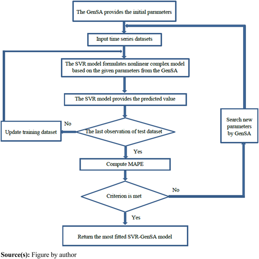
Finally, the most suitable SVR-GenSA model was revealed and utilized to predict container throughput. The flowchart of the SVR-GenSA model is presented in Figure 1.
2.6 The combined approach of seasonal autoregressive integrated moving average, support vector regression and generalized simulated annealing
The combined approach of SARIMA, SVR and GenSA is a complex model that aims at error correction and suitable parameter selection. In the first phase, the SARIMA model is exploited to mimic linear and seasonal patterns of time-series datasets and provides linear components and residuals of the fitted SARIMA model. Afterwards, the SVR–GenSA model is utilized to formulate a complex and nonlinear function with the most suitable input lag and parameters of the SVR model obtained from the GenSA to explain the nonlinear pattern in the residuals. The procedure of the combined approach is demonstrated in the following steps:
2.6.1 The GenSA at the initial artificial temperature randomly generates a set of the initial solutions based on Eq. (10), which are the input lag of the residual series and the parameters of the SVR model. The set of initial solutions is demonstrated in Eq. (16).
2.6.2 The SARIMA model is used to simulate linear and seasonal patterns of time series based on the training dataset by using Eq. (1) to provide the estimated linear component of linear and seasonal patterns and the nonlinear component in residuals of the fitted SARIMA model as illustrated in Eq. (18).
where and are the container throughput observation and the estimated linear component of linear and seasonal patterns at time t. The is the nonlinear component at time t in the residuals of the fitted SARIMA model.
2.6.3 The series of nonlinear components in the residuals of the fitted SARIMA model is reorganized into m columns based on the given input lag, which is obtained from the GenSA as displayed in the following matrix.
2.6.4 The input datasets of nonlinear components, which are equal to the given input lag, are the first m – 1 columns of the matrix for the SVR model.
2.6.5 The target dataset of the nonlinear components is the last column of the matrix for the SVR model.
2.6.6 The fitted SARIMA model based on Eq. (1) is employed to extrapolate a future linear component of linear and seasonal patterns, as demonstrated in Eq. (19).
where f is the fitted SARIMA model. The is the container throughput observation at time t. is the predicted linear component of linear and seasonal patterns at time t +1.
2.6.7 The SVR formulates a complex function based on the given set of parameters corresponding to the kernel hyperparameters for learning relations between both input and output data and provides the future nonlinear component, as demonstrated in Eq. (20).
where f is the fitted SVR model based on the given parameters. The is the nonlinear component at time t in residuals of the fitted SARIMA model. is the predicted nonlinear component at time t + 1. is the given parameters of kernel hyperparameters gained from the GenSA.
2.6.8 The predicted nonlinear component is added to the predicted linear component of linear and seasonal patterns to be the predicted observation of container throughput as presented in Eq. (21).
where is the predicted observation of container throughput at time t + 1. The and are the predicted linear components of linear and seasonal patterns and the predicted nonlinear component at time t + 1, respectively.
2.6.9 If the last observation is not revealed, then repeat steps 2.6.2 to 2.6.8 by adding the presented observation of the test dataset to update the training dataset to provide a rolling forecast.
2.6.10 The predicted observations of container throughput and the actual observations of the container throughput are exploited to compute MAPE. The MAPE is assigned to be the objective function of the GenSA at present.
2.6.11 The GenSA generates new solutions by using Eqs (11)–(13).
2.6.12 Until the criterion of the maximum number of iterations is met, repeat the steps from 2.6.2 to 2.6.11.
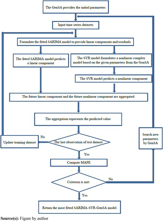
Finally, the most appropriate SARIMA-SVR-GenSA model was demonstrated. Additionally, the most appropriate SARIMA–SVR–GenSA model was used to forecast container throughput. The flowchart of the SARIMA–SVR–GenSA model is demonstrated in Figure 2.
2.7 The proposed model
The proposed model is developed and proposed as a complex model, which exploits the capability of the AHW model to describe the level, trend and seasonality of the time series with exponentially decreasing weights over time and provides estimated smoothing components as well as the smoothing residuals. Although the smoothing residuals of the fitted AHW model can provide a useful series of residuals for the SVR model to build a complex nonlinear function, the smoothing residual series, which is more clear and steady, can support the SVR model to better explain the future residual value. Therefore, the advantage of equal weights from the simple moving average based on the given optimal periods is utilized to adjust the residual series to be a more evident and steady residual series. In the meantime, the GenSA is utilized to search for the most suitable period of the simple moving average in residual adjustment, the most proper input lag of the more smoothing series of residuals and the most appropriate parameters of the SVR model. Consequently, the proposed model focuses on error correction with a more obvious and steady series of residuals and appropriate parameter selection to achieve more accuracy. The process of the proposed model is illustrated as follows:
2.7.1 The initial artificial temperature of the GenSA is set, and the initial solutions are randomly created based on Eq. (10), which corresponds to the moving average period of residual series, input lag of the more smoothing series of residuals and the parameters of the SVR model. The parameter group of the proposed model is expressed in Eq. (22).
2.7.2 The AHW method is exploited to describe the time series based on the training dataset with Eqs (2)–(5). Both the series of smoothing components and the series of residual components are obtained from the fitted AHW model. The mathematical expression is presented in Eqs (23)–(24).
where and are the container throughput observation and the estimated smoothing component of the container throughput observation at time t, respectively. The is the residual component at time t of the fitted AHW model. The f is the fitted AHW model.
2.7.3 The series of residual components is transformed into a more clear and steady series by using a simple moving average with an optimal period, which is obtained from the GenSA.
where is the new more obvious and steady residual value at time t, which is transformed using the simple moving average with the given optimal period.
2.7.4 The new series of more clear and steady residual components is rearranged into columns based on the given input lag, which is obtained from the GenSA as follows.
2.7.5 The given input lag obtained from the GenSA is used to be the input datasets, which are the first m – 1 columns of the matrix regarding the new series of more obvious and steady residual components.
2.7.6 The target dataset is the last column of the matrix regarding the new series of more obvious and steady residual components.
2.7.7 The fitted AHW model with Eqs (2)–(5) is used to predict a smoothing component, as shown in Eq. (26).
where f is the fitted AHW model. is the container throughput observation at time t. The is the predicted smoothing component at time t + 1.
2.7.8 The SVR model based on the given parameters of the kernel hyperparameters received from the GenSA is formulated as a complex function and predicts a residual component, as shown in Eq. (27).
where f is the fitted SVR model with the given set of kernel function parameters. is the more obvious and steady residual component at time t. is the predicted residual component at time t + 1. is the given parameters of kernel hyperparameters obtained from the GenSA.
2.7.9 The predicted observation of container throughput is obtained from the combination of the predicted residual component with the predicted smoothing component, as demonstrated in Eq. (28).
where is the predicted observation of container throughput at time t + 1. The and are the predicted residual component and the predicted smoothing component at time t + 1, respectively.
2.7.10 To repeat steps 2.7.2 to 2.7.9 by aggregating the revealed observation of the test dataset to update the training dataset to provide a rolling forecast until the last observation of the test dataset is presented.
2.7.11 To compare the predicted observations of container throughput with the actual observations of container throughput to calculate MAPE, which is assigned to be the objective function of the GenSA at present.
2.7.12 The set of new solutions is generated from the GenSA using Eqs (11)–(13).
2.7.13 Until the criterion of the maximum number of iterations is met, repeat 2.7.2 to 2.7.12.
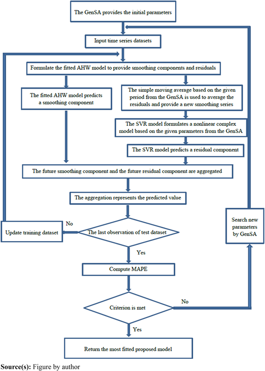
Lastly, the most proper proposed model is presented and exploited to forecast container throughput. The flowchart of the proposed model is illustrated in Figure 3.
3. Dataset and accuracy measures
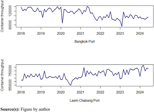
The datasets of container throughput at Thailand’s major ports used in this article were obtained from the Port Authority of Thailand (PAT) (Port Authority of Thailand, 2024), which provides free online information on container throughput at Bangkok and Laem Chabang ports. The datasets of monthly container throughput are time series from January 2018 to June 2024, which are exploited to investigate the forecasting performance of prediction models. Each dataset consists of 78 observations that are separated into three parts, which are roughly 64%, 28% and 8% of all observations for the training data (from January 2018 to February 2022), the test data (from March 2022 to December 2023) and the additional unseen data (from January 2024 to June 2024), respectively. The time-series datasets of Bangkok and Laem Chabang ports are illustrated in Figure 4.
For time series cross-validation, the training dataset is used to formulate predictive functions, and the test dataset is utilized to compute accuracy measures to support the good performance of the proposed models based on three accuracy measures, which are expressed in Eqs (29)–(31).
where and are the actual observation of container throughput and the forecast value of container throughput at time t in the test dataset, respectively.
Moreover, the additional unseen observations, which are not included in either training or test datasets, are used to support the reliable performance of the proposed model to predict additional future observations for other periods in advance. In this regard, the overall datasets of the test datasets and additional unseen datasets are recalculated based on three accuracy measures.
4. Results and discussion
For experiments in this research, the datasets of Bangkok and Laem Chabang ports are investigated by using descriptive statistics for preliminary investigations. The ranges of container throughput dealing with both Bangkok and Laem Chabang ports are presented in Figure 5.
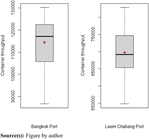
As the results of container throughput are displayed in Figure 5, the summary of container throughput at Bangkok port for minimum, mean, standard deviation and maximum are approximately 86,540 TEU, 114,440 TEU, 10,055 TEU and 130,270 TEU, respectively. Moreover, the summary of container throughput at Laem Chabang port for minimum, mean, standard deviation and maximum are about 548,130 TEU, 696,910 TEU, 58,440 TEU and 828,330 TEU, respectively. Furthermore, the mean of container throughput represents the average in the period from January 2018 to June 2024, where Laem Chabang port is greater than Bangkok port approximately six times. Meanwhile, the standard deviation denotes the amount of variation in the container throughput where Laem Chabang port is greater than Bangkok port approximately six times. In addition, the growth trends of container throughput for both major ports are demonstrated in Figure 6.
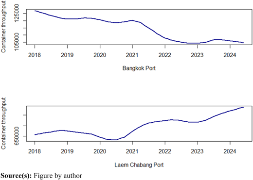
Referencing the results in Figure 6, the trend of container throughput at the Bangkok port likely decreased over time from January 2018 to June 2024. Meanwhile, the trend of container throughput at the Laem Chabang port has likely been increasing from January 2018 to June 2024.
For comparison of forecasting performance, all forecasting models are evaluated by their performance based on three accuracy measures, which are illustrated in Table 1.
The summary of three accuracy measures
| Port | Model | MAE | MAPE | sMAPE |
|---|---|---|---|---|
| Bangkok | ARIMA | 5145.82 | 4.81 | 4.90 |
| AHW | 4285.50 | 3.94 | 3.99 | |
| MHW | 5903.14 | 5.46 | 5.47 | |
| SVR-GenSA | 5723.55 | 5.60 | 5.36 | |
| ARIMA-SVR-GenSA | 4601.91 | 4.23 | 4.35 | |
| Proposed model | 3998.83 | 3.63 | 3.71 | |
| Laem Chabang | ARIMA | 34807.41 | 4.78 | 4.78 |
| AHW | 33487.23 | 4.54 | 4.54 | |
| MHW | 37908.27 | 5.10 | 5.15 | |
| SVR-GenSA | 35208.59 | 4.74 | 4.86 | |
| ARIMA-SVR-GenSA | 34285.45 | 4.72 | 4.70 | |
| Proposed model | 29306.33 | 3.99 | 3.96 |
Source(s): Table by author
According to the results in Table 1, the AHW model provides lower errors than other conventional models for both Bangkok and Laem Chabang ports. In addition, the AHW model can also overcome both the SVR–GenSA model and the ARIMA–SVR–GenSA model based on three accuracy metrics for both datasets. As the results of the above illustration, both datasets of time series tend to have the same magnitude of seasonal patterns over time and have linear patterns as well. Moreover, the exponential smoothing method is well capable of predicting both datasets. However, the proposed model outperforms all other models based on three accuracy measures for all the datasets. Moreover, the combined model of ARIMA, SVR and GenSA can reduce errors compared with the ARIMA model based on three accuracy measures.
In order to support the performance of the proposed model for reliable prediction in other periods, all forecasting models in test datasets are exploited to extrapolate additional unseen observations of container throughput at major ports in Thailand. Therefore, the overall datasets, which consist of the mentioned test data and additional unseen data, are used to evaluate and determine the forecast performance of all models. The summary of three accuracy metrics for the overall datasets of the test and additional unseen data is presented in Table 2.
The summary of three metrics for the datasets of test and additional unseen data
| Port | Model | MAE | MAPE | sMAPE |
|---|---|---|---|---|
| Bangkok | ARIMA | 4900.64 | 4.61 | 4.65 |
| AHW | 4602.75 | 4.28 | 4.32 | |
| MHW | 5822.29 | 5.42 | 5.44 | |
| SVR–GenSA | 5116.64 | 5.00 | 4.80 | |
| ARIMA–SVR–GenSA | 4520.71 | 4.19 | 4.25 | |
| Proposed model | 4367.45 | 4.03 | 4.09 | |
| Laem Chabang | ARIMA | 36267.54 | 4.94 | 4.94 |
| AHW | 33224.93 | 4.47 | 4.49 | |
| MHW | 36211.29 | 4.86 | 4.91 | |
| SVR–GenSA | 47814.96 | 6.30 | 6.57 | |
| ARIMA–SVR–GenSA | 36085.39 | 4.92 | 4.91 | |
| Proposed model | 31603.60 | 4.24 | 4.18 |
Source(s): Table by author
In Table 2, the AHW model still outperforms other conventional models and the SVR–GenSA model for the overall datasets. Although the AHW model provides better results than the ARIMA–SVR–GenSA model for the Laem Chabang port, the AHW model cannot overcome the ARIMA–SVR–GenSA model for the dataset of the Bangkok port. In this regard, the AHW model does not provide good forecasts for the overall datasets in this case. However, the proposed model is still superior to all other models for the overall datasets based on three accuracy metrics.
Furthermore, the forecasts of the proposed model are compared with the actual data of the Bangkok port, which is summarized and demonstrated in Figure 7.
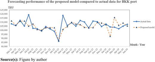
The forecasting performance of the proposed model and actual data for BKK Port
The forecasting performance of the proposed model and actual data for BKK Port
According to the forecasts of the proposed model, the result of the predictions tends to correlate with the actual data of container throughput at the Bangkok port in Thailand.
Moreover, a comparison of the proposed model and the actual data is presented in Figure 8 for container throughput at Laem Chabang port in Thailand.
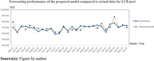
Based on the summary of comparison, the forecasts of the proposed model still correlate with the actual data of container throughput at Laem Chabang port in Thailand.
5. Conclusion
Based on all investigations, the proposed model is superior to all other models with the most accurate forecasts for test datasets in the time-series cross-validation process. Consequently, the proposed model with an optimal smoothing period in residual adjustment can achieve more accuracy. This investigation indicated that residual adjustment based on the optimal smoothing period can provide a more obvious and steady pattern of residuals to enhance the forecast performance of support vector regression. In addition, the proposed model can reduce the risk of uncertainty when dealing with container throughput at major ports in Thailand to support port management decision-making.
Furthermore, the proposed model can still provide superiority to all forecasting models for the overall datasets of the test data and the additional unseen data as well. Consequently, the proposed model can provide reliable forecasts to be a worthwhile guideline for policymakers and operators to develop efficient strategies for port management in Thailand.
Conflict of interest: The author declares that there are no conflicts of interest.
Data availability: The datasets of major ports in Thailand are obtained from Port Authority of Thailand, which provides online information at https://www.port.co.th/cs/internet/internet/index.html

