

Port throughput forecasting is crucial for port planning and regional economic development, while traditional models suffer from poor adaptability to small-sample data, failure to capture periodic and time-varying features and low prediction accuracy. This study aims to develop a more accurate and robust model to realize precise forecasting of China's coastal port throughputs with different time scales and dimensions.
This study proposes a fractional-order time-varying grey Fourier model (FTGFM) by extending the traditional grey model framework. The proposed model integrates a fractional-order accumulation operator, a time-varying correction term and a truncated Fourier series to respectively characterize new-information priority, system dynamic evolution and periodic data fluctuations. The Whale Optimization Algorithm is employed to optimize nonlinear parameters. The effectiveness of the model is evaluated using quarterly data (2017–2025) and monthly data (2023–2025) for four core port throughput indicators, and its performance is compared with six comparative models based on mean absolute percentage error (MAPE), root mean squared error and Theil's U statistic.
Empirical results indicate that FTGFM(1,1) outperforms all benchmark models, with training and testing MAPE both below 3%. It effectively captures the periodic and time-varying trends in port throughput, and forecasts suggest China's port throughput will fluctuate steadily upward in 2026–2027.
The study structurally improves the grey model with a time-varying correction term and embeds Fourier series into grey modeling for port throughput forecasting for the first time, combined with the fractional-order accumulation operator to optimize information processing. The proposed model thus provides an effective new tool for forecasting small-sample time series with periodic and time-varying features.
1. Introduction
Ports, as vital gateways for the circulation of a wide range of elements, are the pivotal nexus between domestic and international markets (Ziran et al., 2022). According to the China Port Operation Analysis Report (2024), China's foreign trade sea transportation volume accounted for 30.1% of the global sea transportation volume, with the year-on-year growth rates of container throughput and foreign trade throughput reaching 4.9% and 9.6%, respectively. Port throughput forecasting exerts a significant influence on the planning of port infrastructure, the improvement of operational efficiency, the determination of investment scale, the formulation of operational strategies and the planning of development strategies (Sun et al., 2024). It also has a far-reaching impact on the economic growth of port cities and the economic development of their hinterland regions (Twrdy and Batista, 2016). As a hub of the logistics network, ports have their throughput influenced by the complex interplay of various factors, which leads to the uncertainty of port throughput and also presents challenges to port forecasting (Liu et al., 2023; Li et al., 2024).
Current research on port data forecasting primarily employs methods such as time series analysis, neural networks and hybrid forecasting models. Time series analysis methods include the cointegration error correction model (Hui Eddie et al., 2004) and the auto regressive integrated moving average (ARIMA) model (Yao, 2021). However, studies by Mokhtar et al. (2022) have found that due to the limited sample size of port throughput data, linear and seasonal ARIMA models exhibit significant errors in forecasting container volumes and freight volumes, especially in short-term predictions. Additionally, some scholars have used single models based on neural network systems to forecast port throughput (Liu et al., 2023), while others have employed hybrid machine learning models composed of multiple models, such as least squares support vector regression (LS-SVR) (Xie et al., 2013) and gated recurrent unit (GRU) neural network, refined with the Adam algorithm (Niu et al., 2018). Nevertheless, single models may face issues of overfitting and local optima, which can affect learning effectiveness. Hybrid models, on the other hand, may easily overlook the influence of exterior determinants and tend to have longer runtime.
Conventional predictive models typically demand voluminous data samples for robust training and validation. Nevertheless, port throughput forecasting is frequently plagued by the scarcity of available historical data, alongside pronounced periodic fluctuations and time-varying dynamics in its evolutionary trajectory (Xie et al., 2013). Intriguingly, the inherent sample characteristics and pervasive data uncertainty associated with port throughput align closely with the core research scope of grey system theory, a methodological framework specifically engineered to address challenges characterized by small datasets and incomplete, ambiguous information. Originated by Deng Julong in 1982, grey system theory is tailored to tackle small-sample and poor-information problems with exceptional efficacy. Among its diverse derivatives, the grey model (GM(1,1)) stands out for its capacity to accurately characterize data variation patterns and conform to the structural attributes of grey systems; accordingly, numerous scholarly efforts have been devoted to refining this model to bolster its practical applicability across real-world scenarios.
Initial conditions and background values constitute two indispensable components that are tightly correlated with parameter estimation, and extensive academic endeavors have targeted the optimization of multivariate grey models from the perspectives of Initial value optimization (Yang et al., 2025), algorithmic improvement (Tang and Zhu, 2025) and background value interpolation coefficient calibration (Wang and Wang, 2023). Beyond methodological tweaks, the intrinsic features of sample data further exert a substantial impact on the predictive error of multivariate grey models, motivating a wealth of studies to customize such models for compatibility with idiosyncratic data evolutionary trends. In the context of nonlinear datasets, Zheng et al. (2021) accounted for the inherent biases stemming from the discrete approximation of differential equations in most prevailing grey sequence models, and subsequently developed an unbiased Nonlinear Grey Bernoulli Model (NGBM(1,1)) to quantify China's hydropower consumption. For capturing seasonal volatility in time series, a spectrum of sophisticated fitting strategies has been proposed, encompassing seasonal buffer operators (Zhou et al., 2020) and seasonal dummy variables (Zhou and Ding, 2021), among other techniques. To accommodate the time-varying traits of sequential data, Qian et al. (2012) developed a grey model containing a time power term GM (1,1, tα) using the concept of grey modeling and the constant c in the grey operation term btα+c, and applied it to predict foundation settlement. Ma and Liu (2017) further innovated a time-delay polynomial grey prediction model (TDPGM(1,1)) to forecast China's natural gas demand with enhanced precision. To forecast port cargo throughput in China, Li et al. (2025) explore policy-driven mechanisms and autoregressive time lag terms, and introduce a novel self-adaptive grey prediction modeling framework.
Grey prediction models have garnered widespread scholarly attention for their superior capability in handling uncertain information and small-sample datasets. Nevertheless, conventional treatments for periodic and seasonal fluctuations in time series, such as seasonal buffer operators and seasonal dummy variables, fail to characterize flexible periodic patterns embedded in the data, thereby compromising the accuracy and reliability of forecasting outcomes. Furthermore, existing empirical validations are mostly confined to single data dimensions, uniform time scales or isolated regional indicators, lacking a comprehensive and multi-dimensional verification framework. Consequently, the generalization performance and practical applicability of such models in port throughput forecasting remain to be further verified.
Notably, port throughput forecasting is featured by sparse datasets, pronounced time-varying dynamics and periodic evolutionary trends, which impose stringent requirements on the descriptive and predictive power of forecasting models. To address these challenges, this paper innovatively develops a fractional-order time-varying grey Fourier model (FTGFM) to better fit the evolutionary trends and fluctuation characteristics of the data. The main contributions of this work are summarized as follows:
Aiming at the inherent time-varying nature of time series, this study structurally improves the traditional fractional grey model (FGM(1,1)) model by innovatively introducing a time-varying correction term. This term accurately characterizes the system's dynamic evolution, and quantifies the dynamic impacts of internal uncertainties.
To capture data periodicity, this paper integrates Fourier series into the grey modeling framework to enhance periodic fluctuation fitting. Fourier series decomposes complex periodic functions into basic sine and cosine components, enabling more accurate simulation and prediction of periodic time series and offering a new method for seasonal trend forecasting.
A multi-dimensional empirical system is constructed to fully validate the proposed FTGFM(1,1) by combining long/short-period datasets and comparing regional and national indicators. Experimental results on port throughput data verify the model's superior prediction accuracy.
2. Methodology
2.1 The existing GM(1,1)
Consider as the original series, formulated as: . Let be the one-order accumulating generation series of , where
The grey model (GM(1,1)) can be expressed as
where denotes the developing coefficient, denotes grey action.
The parameter vector are estimated with the application of the least squares method (LSM).
where, ,
Discretization of the time response Eq. (2) yields
The predicted value of the original sequence is
2.2 Establishment of FTGFM(1,1)
When dealing with time series characterized by periodic fluctuations and time-varying dynamics, adopting an appropriate grey prediction model is critical to achieving effective fitting and forecasting. To address these challenges, a novel grey model, termed the FTGFM and abbreviated as the FTGFM(1,1) model, is proposed in this paper.
2.2.1 Model establishment
The original sequence is represented by a column vector , where is the element of the set and n is the number of the series.
Let be the r-order accumulating generation series of . The fractional order accumulation operator D is delineated thusly:
where,
In the fractional-order accumulation operator, the effective processing of weighted information is achieved by assigning higher weights to the most recent data points, thereby realizing the principle of prioritizing new information. This means that the model gives priority to the latest data points rather than simply averaging all data points. This approach helps enhance the model's sensitivity to recent changes, thereby making the forecasting results more accurate and timely (Wu et al., 2013).
Assume that is given by Definition 4. On the basis of the fractional-order univariate grey prediction model, we incorporate the time-varying term and the truncated Fourier function to establish the FTGFM(1,1) model. The whitening differential equation of the FTGFM(1,1) model is expressed as:
where denotes the development coefficient, represents the time-varying term coefficient, refers to the Fourier coefficient and is an adjustable nonlinear parameter that reflects the sequence frequency to match applications with diverse evolutionary trends and oscillation states. In this work, parameter optimization is adopted to fit the complex periodicity of the sequence. Z denotes the adjustable Fourier order, representing the number of truncated terms, which is correlated with the periodic pattern.
On the one hand, a Fourier series with a small truncation order Z can only represent simple periodic patterns. On the other hand, a model with a higher order enables the fitting of more complex periodic patterns but is accompanied by the risk of overfitting. Therefore, it is crucial to select an appropriate order according to the seasonal time series. An alternative approach is to treat the Fourier truncation order as a parameter and conduct algorithmic optimization to determine its optimal value (Liu et al., 2024).
Fourier series can decompose complex periodic functions into a linear combination of multiple sine and cosine functions with distinct frequencies and amplitudes. Such decomposition capability makes the Fourier series highly suitable for capturing and analyzing the periodic components embedded in data (Xiong et al., 2024).
Let denotes the background value sequence, which is defined as , where
The whitening differential equation is transformed into its discrete form by discretizing Eq (8), and the corresponding grey differential equation is obtained as follows:
2.2.2 Prediction formula of FTGFM (1, 1)
Solving the above equation yields:
Substitute ,
The time response of the FTGFM (1, 1) model is:
Finally,the sequence predicted value can be obtained:
2.3 The solution and optimization of FTGFM (1, 1) model parameters
2.3.1 Structure parameter
As for the FTGFM (1, 1), the development coefficient, Fourier coefficient, and time-varying coefficient must be estimated. The parameter sequence is expressed as , that is,
In the realm of grey prediction, the LSM is the predominant parameter optimization technique. It identifies the optimal development coefficient and grey action by minimizing the squared deviations between simulated and predicted values. And this approach aligns with the scientific principle of simplicity. Consequently, this study employs the LSM to determine the parameter vector . The parameters of the FTGFM (1, 1) model are estimated as follows:
Where,
2.3.2 Estimation of the nonlinear parameter
As for the FTGFM (1, 1), the optimal fractional order r contributes to efficiently addressing new information's priority, the optimal sequence frequency v is conducive to fitting the evolutionary trend and oscillation state of the data and the optimal Fourier truncation order Z is beneficial for fitting complex periodic patterns. Therefore, optimizing these nonlinear parameters of FTGFM (1, 1) can not only augment the forecasting accuracy but also strengthen the model's adaptive and flexible capabilities. We develop a nonlinear constrained optimization model that integrates FTGFM (1, 1) estimated parameters, enabling dynamic identification of true fluctuations. To elaborate, the object function is expressed as the minimum Mean Absolute Percentage Error (MAPE) for true data and estimated outcomes (see Eq. (15)). Under constraints, Whale Optimization Algorithm (WOA) serves to optimize the parameters r and v as real numbers, while performing integer optimization for Z, thereby achieving accurate forecasting. Specifically, the search ranges of parameters r, v and Z are set to [0,2], [−10,10] and [0,10] respectively; the population size is set to 50; and the maximum number of iterations is set to 200. The objective function and constraints of WOA are shown in the equations.
2.4 Framework of the model
2.4.1 Criteria for validation
To assess the model's prediction exactness and examine relative and absolute errors of predicted and real values, this study selects four evaluation indicators to evaluate the model's effectiveness, involving APE, MAPE, root mean squared error (RMSE) and Theil U statistic (U). The formulas are presented in the following manner:
where, denotes the simulated outcomes obtained by recursion of Eq.(12), denotes the real values.
2.4.2 Modeling process
The detailed modeling process is presented as follows:
Step 1: The system behavior sequence is determined via relevant literature and validated data sources. The dataset is split into training and testing subsets for model building and accuracy validation. To fit the exponential growth trend, r-order fractional accumulation is applied to the raw data to generate the accumulated sequence and boost model adaptability.
Step 2: Model coefficients are estimated via the OLS method to minimize the sum of squared deviations between estimated and actual values, ensuring parameters reflect the system's internal structure and improve fitting accuracy.
Step 3: To boost prediction accuracy, the WOA is adopted to fine-tune hyperparameters (fractional accumulation order and power exponent), which are vital for capturing data dynamics. The FTGFM(1,1) model is then built with the optimized hyperparameters.
Step 4: Time Response Derivation. Using the parameters obtained in Step3, the time response function of the FTGFM (1, 1) model is formulated to generate the predicted accumulated sequence. The purpose of this step is to reconstruct the system's dynamic evolution over time. Subsequently, the inverse accumulation process is performed to obtain the final forecast values in their original scale.
Step 5: The predicted values are used to calculate performance metrics, including MAPE, RMSE and Theil's Inequality Coefficient (U), enabling the comparison of prediction performance and robustness with other benchmark models.
3. Verification and application
3.1 Research design
To verify the effectiveness of the proposed port trade forecasting model and achieve accurate prediction of future port throughput data, multi-dimensional core port throughput indicators are selected to construct the research dataset. Specifically, the indicators are defined as follows: coastal cargo throughput (CCgT) refers to the total quantity of all types of cargo handled at coastal ports within a specified time interval, which comprehensively reflects the cargo distribution capacity and regional logistics hub status of coastal ports; coastal foreign trade cargo throughput (CFTCT) denotes the total volume of import and export goods loaded and unloaded through coastal ports during a certain period, which directly characterizes the port's foreign trade service capacity and linkage level with the global industrial chain; national port cargo throughput (NPCT) represents the total amount of cargo handled by all ports across the country within a defined period, which reflects the overall development scale of the national port system; coastal container throughput (CCnT) refers to the total number of containers handled at coastal ports within a specified interval, which measures the port's containerized transportation level and international shipping hub capacity.
Quarterly data spanning 2017 to 2025 are adopted for coastal cargo throughput and CFTCT, aiming to depict the long-term evolutionary trends of the indicators. Monthly data covering 2023–2025 are selected for NPCT and coastal container throughput, to capture short-term fluctuation characteristics and conduct comprehensive predictive analysis of regional and national port development levels (data sourced from the wind database). The dataset is divided into training and testing subsets according to data frequency. For the quarterly data of coastal cargo throughput and CFTCT, 28 consecutive quarterly samples from 2017 to 2023 are utilized as the training set to complete the optimal estimation of model parameters and deeply mine long-term trend features, while 8 quarterly samples from 2024 to 2025 are employed as the testing set to verify the extrapolation accuracy and result robustness of the model. For the monthly data of NPCT and coastal container throughput, 24 consecutive monthly samples from 2023 to 2024 are applied as the training set to effectively fit the short-term fluctuation rules of the indicators and 12 monthly samples in 2025 are used as the testing set to test the model's prediction capability and generalization performance for high-frequency data.
This study combines long- and short-cycle data, as well as compares regional and national indicators, providing rigorous and scientific data support for model effectiveness verification and future port throughput data prediction.
3.2 Application of quarterly port data
3.2.1 Prediction performance analysis of CCgT and CFTCT
The raw data of CCgT and CFTCT are divided into training and testing sets, and the WOA is adopted to optimize the real numbers and , while the Fourier truncation order is optimized as an integer. The FTGFM(1,1) model is then evaluated against six competing models in terms of prediction performance, based on the sequence length that achieves the highest accuracy. For CCgT, the optimal parameters are determined as and . For CFTCT, the optimal parameters are determined as and . Subsequently, simulations and predictions for CCgT and CFTCT are carried out based on the time response function and estimated parameters. Finally, the upper and lower bounds of errors are determined using the specified equations, and the average relative error is calculated accordingly.
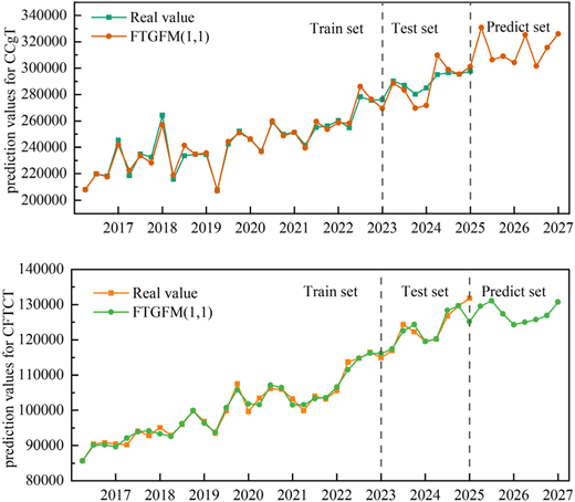
For validation purposes, the model's forecasting outcomes were contrasted with results from other models, including back propagation neural network (BPNN), ARIMA, GM(1,1), fractional time-varying grey model (FTGM(1,1)) and seasonal grey model (SGM(1,1)) models. Table 1 provides the prediction results for the test set. The simulation curve of the new model is depicted in Figure 1. The forecast curve roughly corresponds to the actual value curve, and fits the periodicity and nonlinearity of the original sequence very well. Compared with the real values, the predicted values show excellent fitting accuracy.
Testing set outcomes among six models in CCgT and CFTCT
| Quarter | Real value | FTGFM(1,1) | BPNN | ARIMA | GM(1,1) | FTGM(1,1) | SGM(1,1) |
|---|---|---|---|---|---|---|---|
| CCgT (Ten thousand tons) | |||||||
| 2024–1 | 290,172 | 288545.38 | 278236.55 | 265989.92 | 269812.27 | 274179.10 | 258690.98 |
| 2024–2 | 287,027 | 283370.65 | 278322.85 | 276291.72 | 271676.56 | 278771.99 | 270561.47 |
| 2024–3 | 280,269 | 269636.43 | 278315.49 | 269855.87 | 273545.05 | 283764.46 | 276942.88 |
| 2024–4 | 285,000 | 271698.75 | 278302.95 | 279944.29 | 275417.76 | 289190.96 | 274762.71 |
| 2025–1 | 295,089 | 309784.62 | 278297.33 | 273719.09 | 277294.69 | 295088.99 | 266359.50 |
| 2025–2 | 296,504 | 298894.91 | 278295.51 | 283599.54 | 279175.85 | 301499.26 | 278581.86 |
| 2025–3 | 295,405 | 295404.82 | 278295.06 | 277579.66 | 281061.26 | 308466.04 | 285152.45 |
| 2025–4 | 297,710 | 301190.92 | 278294.99 | 287257.42 | 282950.91 | 316037.43 | 282907.65 |
| CFTCT (Ten thousand tons) | |||||||
| 2024–1 | 117,001 | 117385.78 | 113733.15 | 114127.51 | 114159.86 | 120170.34 | 107354.28 |
| 2024–2 | 124,352 | 122542.43 | 113261.11 | 114942.02 | 115155.35 | 121926.15 | 117908.55 |
| 2024–3 | 122,261 | 124341.13 | 113040.71 | 115890.06 | 116155.14 | 123747.89 | 118719.52 |
| 2024–4 | 119,658 | 119545.53 | 112944.35 | 116838.10 | 117159.24 | 125638.27 | 123924.56 |
| 2025–1 | 120,204 | 120203.99 | 112903.53 | 117786.14 | 118167.68 | 127600.10 | 111414.55 |
| 2025–2 | 126,760 | 128341.62 | 112886.52 | 118734.18 | 119180.47 | 129636.27 | 122367.99 |
| 2025–3 | 129,668 | 129668.59 | 112879.50 | 119682.21 | 120197.64 | 131749.77 | 123209.64 |
| 2025–4 | 131,789 | 125135.86 | 112876.62 | 120630.25 | 121219.20 | 133943.69 | 128611.54 |
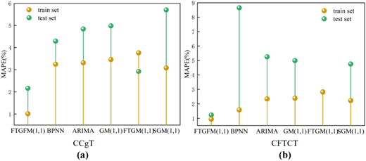
From the perspective of error distribution, Table 2 and Figure 2 present the MAPE, RMSE and Theil's U statistic for all prediction models in both training and testing phases, and the results show that the FTGFM(1,1) model achieves the lowest values of these three indicators among BPNN, ARIMA, GM(1,1), FTGM(1,1) and SGM(1,1) models, reflecting its distinct superiority in simulation and forecasting performance. In the training phase, FTGFM(1,1) yields very low errors for both CCgT and CFTCT datasets. In the forecasting (testing set) phase, for the CCgT dataset, FTGFM(1,1) obtained a MAPE of 2.16%, an RMSE of 8214.20 and a U of 0.03; for the CFTCT dataset, the MAPE was 1.23%, the RMSE was 2610.78 and the U was 0.02. These are the lowest values among all comparison models for both datasets, demonstrating satisfactory performance in simulating and forecasting the relevant time-series data.
MAPE, RMSE and U among six models in CCgT and CFTCT
| Set | Index | FTGFM(1,1) | BPNN | ARIMA | GM(1,1) | FTGM(1,1) | SGM(1,1) |
|---|---|---|---|---|---|---|---|
| CCgT | train set | ||||||
| MAPE | 1.01 | 3.25 | 3.31 | 3.46 | 3.76 | 3.08 | |
| RMSE | 3486.32 | 10620.73 | 10168.62 | 12073.44 | 12104.02 | 8999.98 | |
| U | 0.01 | 0.04 | 0.04 | 0.05 | 0.05 | 0.04 | |
| test set | |||||||
| MAPE | 2.16 | 4.29 | 4.84 | 4.98 | 2.92 | 5.70 | |
| RMSE | 8214.20 | 13919.80 | 15346.86 | 15114.82 | 10518.67 | 18870.76 | |
| U | 0.03 | 0.05 | 0.06 | 0.05 | 0.04 | 0.07 | |
| CFTCT | train set | ||||||
| MAPE | 0.94 | 1.58 | 2.34 | 2.39 | 2.81 | 2.23 | |
| RMSE | 1175.24 | 2147.67 | 3048.10 | 3074.22 | 3922.68 | 2960.80 | |
| U | 0.01 | 0.02 | 0.03 | 0.03 | 0.04 | 0.03 | |
| test set | |||||||
| MAPE | 1.23 | 8.65 | 5.26 | 4.99 | 2.82 | 4.76 | |
| RMSE | 2610.78 | 11984.78 | 7414.86 | 7063.84 | 3966.35 | 6261.73 | |
| U | 0.02 | 0.11 | 0.06 | 0.06 | 0.03 | 0.05 |
3.2.2 Analysis of prediction results
Predictions for these two indicators across eight quarters of 2026 are generated via the model, and both show a steady fluctuating upward trend as depicted in Figure 1 and Table 3. In 2026, CCgT and CFTCT will maintain overall steady growth, with positive quarter-on-quarter changes in most quarters, which aligns well with the model's verified low error and high stability. Specifically, CCgT climbs gradually from its Q1 2026 baseline and stays at a high level quarter by quarter; CFTCT also rises continuously with minor inter-quarter fluctuations, presenting favorable growth continuity. These results validate the model's accuracy in capturing time-series trends and reflect the resilience of the corresponding business sectors.
Prediction results of FTGFM(1,1) in CCgT and CFTCT
| Quarter | CCgT | CFTCT |
|---|---|---|
| 2026–1 | 330757.42 | 129558.70 |
| 2026–2 | 306423.13 | 131085.62 |
| 2026–3 | 309038.66 | 127371.53 |
| 2026–4 | 304257.30 | 124295.55 |
| 2027–1 | 325162.83 | 124977.35 |
| 2027–2 | 301625.60 | 125717.47 |
| 2027–3 | 315534.72 | 126873.11 |
| 2027–4 | 326014.33 | 130718.30 |
The continuous growth of CCgT and CFTCT is driven by the combined effects of multiple factors. First, the restructuring of the global industrial chain and the recovery of international trade have underpinned the expansion of business volume, laying a solid foundation for the upward trend of the indicators. Second, technological advancements, including port digital transformation and the deployment of intelligent handling equipment, have greatly enhanced operational efficiency and service capacity, providing robust technical support for sustained growth.
The quarterly forecasts for CCgT and CFTCT hold unique value as a risk early-warning and strategic alignment tool for stakeholders across the maritime trade ecosystem. For port operators and infrastructure investors, the identified quarterly fluctuation patterns enable forward-looking allocation of deep-water berths, storage facilities and multimodal transport corridors. This allows stakeholders to pre-empt capacity bottlenecks during high-demand quarters, optimize resource utilization in slower periods and prioritize investments in high-potential growth segments, thereby improving asset efficiency and long-term operational sustainability. From a trade and macroeconomic governance perspective, these forecasts serve as critical leading indicators for assessing the trajectory of coastal foreign trade and formulating targeted stabilization policies. The steady growth of CFTCT signals sustained external demand, providing empirical evidence for policymakers to refine export support measures, streamline customs clearance procedures and strengthen regional trade cooperation. Meanwhile, the consistent expansion of CCgT underscores the vitality of domestic and international circulation, helping authorities align port development with broader industrial upgrading and regional economic integration goals, ultimately fostering more resilient and high-quality growth in coastal economic zones.
3.3 Application of monthly port data
3.3.1 Prediction performance analysis of NPCT and CCnT
The raw data of NPCT and CCnT are divided into training and testing sets, and the WOA is adopted to optimize the real numbers and , while the Fourier truncation order is optimized as an integer. The FTGFM(1,1) model is then evaluated against six competing models in terms of prediction performance, based on the sequence length that achieves the highest accuracy. For NPCT, the optimal parameters are determined as and . For CCnT, the optimal parameters are determined as and . Subsequently, simulations and predictions for CCgT and CFTCT are carried out based on the time response function and estimated parameters. Finally, the upper and lower bounds of errors are determined using the specified equations, and the average relative error is calculated accordingly.
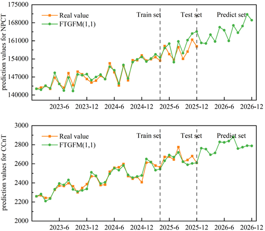
For validation purposes, the model's forecasting outcomes were contrasted with results from other models, including BPNN, ARIMA, GM(1,1), FTGM(1,1) and SGM(1,1) models. Table 4 provides the prediction results for the testing set.The simulation curve of new model is depicted in Figure 3. The forecast curve roughly corresponds to actual value curve, and fits the periodicity and nonlinearity of the original sequence very well. Compared with the real values, the predicted values show excellent fitting accuracy.
Testing set outcomes among six models in NPCT and CCnT
| Month | Real value | FTGFM(1,1) | BPNN | ARIMA | GM(1,1) | FTGM(1,1) | SGM(1,1) |
|---|---|---|---|---|---|---|---|
| NPCT (Ten thousand tons) | |||||||
| 2025–1 | 153,368 | 152970.40 | 152794.15 | 151330.00 | 152601.46 | 161453.33 | 150242.10 |
| 2025–2 | 153,870 | 154125.88 | 152626.72 | 152650.96 | 153050.48 | 162009.91 | 150701.00 |
| 2025–3 | 154,690 | 155765.49 | 152232.94 | 152864.91 | 153500.82 | 162564.65 | 150532.32 |
| 2025–4 | 153,341 | 154570.81 | 151633.02 | 153307.41 | 153952.49 | 163117.80 | 151475.79 |
| 2025–5 | 158,993 | 158174.91 | 151073.50 | 153702.73 | 154405.48 | 163669.59 | 151875.22 |
| 2025–6 | 155,856 | 159909.28 | 150741.84 | 154107.79 | 154859.81 | 164220.20 | 152339.11 |
| 2025–7 | 153,729 | 152757.80 | 150594.95 | 154510.83 | 155315.47 | 164769.83 | 152168.59 |
| 2025–8 | 158,545 | 160780.00 | 150538.36 | 154914.29 | 155772.48 | 165318.62 | 153122.32 |
| 2025–9 | 154,030 | 156221.51 | 150517.74 | 155317.67 | 156230.83 | 165866.72 | 153526.09 |
| 2025–10 | 156,837 | 161282.00 | 150510.39 | 155721.06 | 156690.53 | 166414.28 | 153995.02 |
| 2025–11 | 161,452 | 163809.80 | 150507.79 | 156124.45 | 157151.58 | 166961.40 | 153822.65 |
| 2025–12 | 158,865 | 164604.15 | 150506.87 | 156527.84 | 157613.99 | 167508.21 | 154786.75 |
| CCnT (Ten thousand standard containers) | |||||||
| 2025–1 | 2,612 | 2650.61 | 2544.51 | 2555.25 | 2540.89 | 2615.58 | 2554.35 |
| 2025–2 | 2,618 | 2617.63 | 2581.73 | 2567.41 | 2552.56 | 2618.00 | 2590.58 |
| 2025–3 | 2,581 | 2532.81 | 2596.99 | 2579.57 | 2564.29 | 2620.37 | 2587.53 |
| 2025–4 | 2,566 | 2544.82 | 2602.16 | 2591.72 | 2576.08 | 2622.69 | 2632.27 |
| 2025–5 | 2,672 | 2631.55 | 2603.81 | 2575.58 | 2587.92 | 2624.97 | 2601.67 |
| 2025–6 | 2,675 | 2691.86 | 2604.31 | 2616.04 | 2599.81 | 2627.20 | 2638.57 |
| 2025–7 | 2,644 | 2669.87 | 2604.47 | 2628.19 | 2611.76 | 2629.38 | 2635.46 |
| 2025–8 | 2,775 | 2719.03 | 2604.52 | 2640.35 | 2623.76 | 2631.53 | 2681.03 |
| 2025–9 | 2,622 | 2622.00 | 2604.53 | 2652.51 | 2635.82 | 2633.62 | 2649.87 |
| 2025–10 | 2,640 | 2590.11 | 2604.54 | 2664.67 | 2647.93 | 2635.68 | 2687.46 |
| 2025–11 | 2,681 | 2603.77 | 2604.54 | 2676.82 | 2660.10 | 2637.70 | 2684.29 |
| 2025–12 | 2,609 | 2610.97 | 2604.54 | 2688.98 | 2672.32 | 2639.67 | 2730.70 |
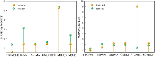
From the perspective of error distribution, Table 5 and Figure 4 present the MAPE, RMSE and Theil's U statistic for all prediction models in both training and testing phases, and the results show that the FTGFM(1,1) model achieves the lowest values of these three indicators among BPNN, ARIMA, GM(1,1), FTGM(1,1) and SGM(1,1) models, reflecting its distinct superiority in simulation and forecasting performance. In the model fitting (training set) phase, for the NPCT dataset, FTGFM(1,1) achieved a MAPE of 0.59%, an RMSE of 984.77 and a U of 0.01; for the CCnT dataset, the MAPE was 0.91%, the RMSE was 25.24 and the U was 0.01. In the forecasting (testing set) phase, for the NPCT dataset, FTGFM(1,1) obtained a MAPE of 1.37%, an RMSE of 3335.17 and a U of 0.02; for the CCnT dataset, the MAPE was 1.18%, the RMSE was 47.98 and the U was 0.01. These are the lowest values among all comparison models for both datasets, demonstrating relatively satisfactory performance in simulating and forecasting the relevant time-series data.
MAPE, RMSE and U among six models in NPCT and CCnT
| Set | Index | FTGFM(1,1) | BPNN | ARIMA | GM(1,1) | FTGM(1,1) | SGM(1,1) |
|---|---|---|---|---|---|---|---|
| NPCT | train set | ||||||
| MAPE | 0.59 | 1.42 | 1.37 | 1.43 | 5.30 | 1.41 | |
| RMSE | 984.77 | 2415.48 | 2331.10 | 2376.65 | 8273.80 | 2321.57 | |
| U | 0.01 | 0.02 | 0.02 | 0.02 | 0.06 | 0.02 | |
| test set | |||||||
| MAPE | 1.37 | 3.13 | 1.41 | 1.62 | 5.37 | 2.38 | |
| RMSE | 3335.17 | 7207.87 | 3364.43 | 2743.45 | 10522.21 | 5227.56 | |
| U | 0.02 | 0.04 | 0.02 | 0.01 | 0.05 | 0.03 | |
| CCnT | train set | ||||||
| MAPE | 0.91 | 1.41 | 2.15 | 2.23 | 9.00 | 2.20 | |
| RMSE | 25.24 | 38.69 | 56.82 | 57.83 | 243.23 | 57.52 | |
| U | 0.01 | 0.02 | 0.03 | 0.03 | 0.10 | 0.03 | |
| test set | |||||||
| MAPE | 1.18 | 1.99 | 1.81 | 1.91 | 1.38 | 1.79 | |
| RMSE | 47.98 | 83.02 | 75.44 | 79.87 | 64.27 | 72.06 | |
| U | 0.01 | 0.03 | 0.02 | 0.03 | 0.02 | 0.02 | |
3.3.2 Analysis of prediction results
Based on the systematic comparison of prediction performance among various models in the preceding section, the FTGFM(1,1) model achieves the highest accuracy and stability in the monthly forecasting of NPCT and coastal container throughput (CCnT). The 12-month forecast values for 2026 generated by this model (see Table 6 and Figure 3) reveal that both throughput indicators exhibit a fluctuating yet steady upward trend, which is highly consistent with the periodic patterns of historical data. Specifically, the annual range of NPCT in 2026 is 159990.41–171266.74, climbing gradually from 160183.19 in January to 168992.75 in December and peaking in November. CCnT fluctuates within the range of 2694.23–2837.87, starting at 2763.15 in early January and closing at 2787.55 at the end of the year, with its annual high recorded in July. This moderate growth trend not only reflects the seasonal patterns of port operations but also validates the FTGFM(1,1) model's ability to accurately capture both trends and fluctuations.
Prediction results of FTGFM(1,1) in NPCT and CCnT
| Month | NPCT | CCnT |
|---|---|---|
| 2026–1 | 160183.19 | 2763.15 |
| 2026–2 | 159990.41 | 2753.47 |
| 2026–3 | 163379.42 | 2694.23 |
| 2026–4 | 160725.53 | 2714.13 |
| 2026–5 | 166261.79 | 2829.04 |
| 2026–6 | 165087.50 | 2824.49 |
| 2026–7 | 160988.53 | 2837.87 |
| 2026–8 | 166999.17 | 2880.45 |
| 2026–9 | 164145.17 | 2759.37 |
| 2026–10 | 166750.92 | 2773.52 |
| 2026–11 | 171266.74 | 2789.39 |
| 2026–12 | 168992.75 | 2787.55 |
From the perspective of driving logic, the recovery of global trade and the resilience restoration of cross-border supply chains provide demand-side support for NPCT and CCnT. Technological innovations such as port automation upgrades and the popularization of intelligent dispatching systems release operational efficiency from the supply side, effectively underpinning throughput expansion. Coupled with the coordinated development of domestic and international economic cycles, these factors jointly drive the steady growth of national port throughput in 2026.
The above monthly forecast results for NPCT and CCnT in 2026 can provide key quantitative references for port operations, logistics planning and macroeconomic decision-making. On one hand, port operators can deploy quay cranes, storage yard capacity and collection-distribution transportation resources in advance based on the monthly fluctuation characteristics, so as to alleviate peak-season operational pressures, optimize off-season resource allocation, reduce operational costs and improve service efficiency. On the other hand, logistics and supply chain enterprises can rationally plan route layout, cabin allocation and warehouse network construction based on the steady growth trend, respond to changes in trade flow in advance and enhance supply chain resilience and risk resistance. From a macro governance standpoint, these forecasts provide empirical evidence for transportation and commerce authorities to refine port development strategies, upgrade intermodal logistics systems and design trade-stabilizing policies. They help pinpoint high-pressure months for infrastructure investment and channel security, while serving as leading indicators to assess global trade recovery and monitor progress in the dual circulation of domestic and international economies–ultimately fostering more precise alignment between port development and broader macroeconomic goals.
4. Conclusions
Ports throughput forecasting serves as the foundation for port structure optimization and infrastructure construction. Accurate prediction of future ports throughput facilitates the advancement of transportation construction in port cities and contributes significantly to the sustainable development of the transportation industry. This study focuses on the quarterly and monthly variations of China's ports throughput, adopting a novel grey prediction model capable of capturing periodic data fluctuations for forecasting. The proposed model delivers superior prediction performance.
To incorporate more uncertain information, this paper presents the FTGFM(1,1) model applicable to prediction, which alleviates the errors of the traditional GM(1,1) model regarding the new information priority principle and data feature fitting to a certain extent. In accordance with the new information priority rule in grey system theory, a fractional-order accumulation operator is introduced to construct the r-AGO sequence. Furthermore, the model integrates Fourier function terms and time-varying terms, exhibiting greater advantages in forecasting sequences with periodic and time-varying trends, especially seasonal data.
To verify the effectiveness and practicability of the model, the FTGFM(1,1) is employed to conduct forecasting via four application cases: quarterly data of coastal cargo throughput and CFTCT, as well as monthly data of NPCT and coastal container throughput. The multi-dimensional design can effectively verify the stability, adaptability and generalization ability of the proposed FTGFM(1,1) model under different data frequencies and spatial scales, which provides a referable modeling paradigm for port throughput forecasting with multi-scenario and multi-scale characteristics. The proposed model is compared with BPNN, ARIMA, GM(1,1), FTGM(1,1) and SGM(1,1) models. The results demonstrate that the FTGFM(1,1) can accurately predict sequences with time-varying and periodic trends, with MAPE values of both the training and testing sets below 3, outperforming the other five models in terms of accuracy and fluctuation similarity.
The optimized model in this study performs better than other benchmarks in port throughput forecasting, indicating that the improved grey prediction framework can also be applied to forecast data with variable characteristics. Admittedly, this research still has limitations. In many practical systems, the relationships between variables are not immediately reflected but feature a certain time-delay effect. Therefore, the time-delay effect may be considered in the construction of prediction models in future work, enabling the model to capture future variable changes more accurately.
