Skip to article sections
Purpose

This study aims to improve the accuracy of transportation delay prediction in supply chains by developing a machine learning-based model. The proposed approach addresses the challenges of parameter tuning and feature selection by integrating the Firefly Algorithm with decision tree regression, helping businesses mitigate the negative impacts of delivery uncertainties.

Design/methodology/approach

The study employs a hybrid machine learning approach using decision tree regression enhanced by the Firefly Algorithm for both parameter optimization and feature selection. The model is trained and tested on the publicly available Dataco Smart Supply Chain dataset, consisting of 180,519 transaction records. The performance of the proposed method is compared with four baseline regression techniques: SVR, MLPRegressor, Lasso Regression and Bayesian Ridge.

Findings

The proposed method significantly outperformed the baseline models across all evaluation metrics. It achieved an R2 score of 0.987, the highest among the tested models and reported the lowest errors in MAE, MSE and MSLE. The Firefly Algorithm effectively enhanced prediction performance by selecting relevant features and tuning model parameters, leading to improved generalizability and reduced overfitting.

Originality/value

This research introduces a novel integration of the Firefly Algorithm with decision tree regression for delay prediction in logistics, demonstrating superior accuracy and computational efficiency. The approach offers practical value for real-world logistics environments by enabling more reliable delivery time forecasts without the need for high-performance computing infrastructure. It also fills a critical gap in the literature by showing the benefits of combining feature selection and hyperparameter optimization in a single workflow.

Global supply chains have become essential to modern commerce, facilitating international trade and business operations (Hathikal et al., 2020). A critical aspect of supply chain management is the timely transportation of goods, as delays can lead to significant financial losses, damaged business relationships, and decreased customer satisfaction (Al-Saghir, 2022). Transportation delays can arise from various factors, including traffic, weather disruptions, customs issues, or technological limitations (Polim et al., 2017). As the global market grows, minimizing these delays becomes increasingly important.

Efficiently managing transportation delays is vital for enhancing operational performance and ensuring customer satisfaction. Predictive models that leverage transport tracking data are key in this context, helping businesses identify delay scenarios and forecast delivery times more accurately. These models provide critical insights, aiding decision-making processes and reducing supply chain costs (Balster et al., 2020). Key factors such as shipment date, weather conditions, and traffic status significantly influence the accuracy of these predictions.

In recent years, machine learning techniques have proven effective in predicting transportation delays by analyzing complex data and identifying patterns within large datasets. These algorithms can model the intricate relationships between variables like traffic disruptions and weather conditions, enabling better predictions of delivery times (Al-Saghir, 2022). By integrating advanced techniques, businesses can mitigate the impact of unpredictable delays on their operations (Jain, 2018).

The costs of transportation delays, including storage fees, depreciation of goods, and customer dissatisfaction, can be substantial for businesses (Balster et al., 2020). Therefore, accurately predicting delivery durations is essential to proactively address potential disruptions. Reliable delay predictions allow companies to take preventive measures, avoid unnecessary costs, and improve overall customer experiences (Jain, 2018).

This study proposes a machine learning-based model for predicting transportation delays in goods shipments. By utilizing historical tracking data, the model aims to enhance prediction accuracy, helping businesses better understand delay patterns and make more informed decisions.

Currently, accurately predicting transportation delays is one of the major challenges in supply chain management due to various complexities such as traffic conditions, weather status, and customs issues. This problem can lead to customer dissatisfaction and increased costs for companies. Given the importance of precise delay prediction, the use of artificial intelligence and machine learning models can provide effective solutions to address these challenges.

The main research questions in this study are as follows:

  1. How can machine learning models be used to accurately predict transportation delays?

  2. What role do optimization algorithms such as the Firefly Algorithm play in tuning model parameters and feature selection, and how do they affect model performance?

Despite numerous studies on predicting transportation delays, most existing models have not focused adequately on optimizing model parameters or feature selection. This issue results in reduced prediction accuracy and misalignment of models with varying conditions. Therefore, there is a need for approaches that can more precisely adjust model parameters and identify effective features using optimization algorithms such as the Firefly Algorithm. This research gap is particularly evident in the integration of optimization algorithms with machine learning models for predicting transportation delays.

This research proposes a new model for predicting transportation delays that utilizes the Firefly Algorithm for tuning the decision tree model parameters and selecting relevant features. The proposed approach specifically uses the Firefly Algorithm as a tool for optimizing prediction models, leading to significant improvements in prediction accuracy and model performance. This study also compares the performance of this model with basic methods and demonstrates the impact of the Firefly Algorithm in improving transportation delay prediction results.

In recent years, predicting transportation delays in supply chains has gained significant attention due to its impact on operational efficiency, cost management, and customer satisfaction. Numerous studies have explored the application of machine learning and data-driven methods for predicting delays, focusing on factors such as traffic, weather disruptions, and logistical inefficiencies. These studies have provided valuable insights into the development of predictive models and optimization of supply chain management.

The research by Al-Saghir (2022) focused on predicting late deliveries using machine learning and the Dataco supply chain data. Logistic regression was found to be the most effective model for this task. The study by Amellal et al. (2023) proposed a framework for time prediction and anomaly detection using the LSTM model and Convolutional Neural Network (CNN), achieving high accuracy with data collected from an ERP system for a major car distributor in Morocco. Erkmen et al. (2022) used Support Vector Machine (SVM) and a backward-looking approach to improve delivery time prediction accuracy by 59.12%. (Mahajan et al., 2022) applied multiple regression models to predict shipment arrival times using both internal data from a company and maritime traffic data, achieving an accuracy of 89%.

Barros et al. (2023) designed a decision support system for delivery time estimation using regression models and data mining techniques. The Random Forest model performed best, reducing delivery time errors by 18–24%. Bani-Mustafa et al. (2018) identified key factors influencing transportation service delivery time in Saharan Algeria, such as the supplier, cargo, and departure port, using a multiple regression model. Servos et al. (2019) used machine learning algorithms such as ExtraTrees, AdaBoost, and SVR to predict travel time in multimodal transportation, with SVR achieving the best performance.

Kandula et al. (2021) introduced a decision support framework for improving delivery success rates in e-commerce. This framework predicted delivery time windows and reduced costs by 10.2%. (Alnahhal et al., 2021; Daneshvar et al., 2025) applied machine learning techniques such as linear and logistic regression to predict dynamic delay times in custom supply chains, with reasonable accuracy. Hathikal et al. (2020) proposed a prediction model for ocean-imported shipments using multinomial logistic regression, with data collected from an industrial company. Lochbrunner and Witschel (2022) explored combining machine learning models with human knowledge for delivery time prediction, finding that a purely machine learning model performed better than the hybrid model.

The study by Pineda-Jaramillo et al. (2023) demonstrated that the LightGBM model outperformed other models, such as SVM and CatBoost, for predicting delays. Huang et al. (2020) developed a deep learning model combining 3D CNN, LSTM, and FCNN to predict train delays, achieving high accuracy through the use of spatiotemporal features. The research by Pineda-Jaramillo and Viti (2023) showed that the CatBoost model outperformed others in predicting railway delay times. Finally, Shi et al. (2021) proposed a combined XGBoost and Bayesian optimization model for predicting train arrival delays, achieving excellent results in terms of accuracy and RMSE. A summary of some of the methods reviewed in this study is given in Table 1.

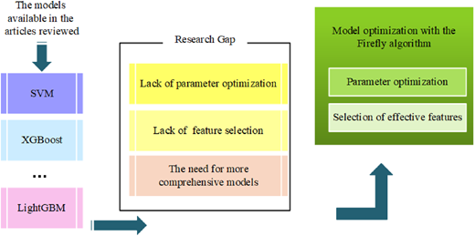
Figure 1 depicts the conceptual framework of this study, positioning it within the context of existing transportation delay prediction models. It identifies research gaps in current methods, particularly in parameter optimization and feature selection, which lead to reduced prediction accuracy. This study uses the Firefly Algorithm to address these gaps and provide more accurate and adaptable models.

In this study, a prediction system for forecasting transportation delay duration based on the combination of machine learning techniques is presented. The proposed system in this research utilizes a combination of the Firefly Algorithm and Decision Tree methods for prediction. In the proposed system, initially, preprocessing processes are applied to the dataset to prepare the data for the application of the learning model. Next, the dataset is divided into training and testing datasets.

The core learning model in this study is the Decision Tree method. To enhance the performance of the machine learning approach, the process of tuning the Decision Tree parameters and selecting effective features is carried out with the help of the Firefly Algorithm.

The Firefly algorithm has been chosen due to its unique characteristics, inspired by the behavior of fireflies in nature. This algorithm can effectively search through a complex parameter space and move towards optimal regions. The natural behavior of fireflies, which are attracted to light, allows the Firefly algorithm to quickly converge to optimal combinations of parameters and features. This feature is particularly useful in optimizing parameters for complex models like decision trees and selecting effective features, as it can significantly improve prediction accuracy and prevent issues like overfitting.

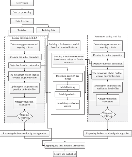
Compared to other hybrid methods, such as genetic algorithms or simulated annealing, the Firefly algorithm offers greater speed and accuracy in exploring the parameter space. Other algorithms may require more time to find the optimal solution or may fail to provide better results due to inefficient searching. Therefore, the use of Firefly, with its more effective search capability and faster optimization of parameters and features, enhances the model's performance and distinguishes it from other hybrid methods. The relationship between the components of the proposed system is given in Figure 2.

The overall procedure is structured as follows:

  1. Receive the data.

  2. Preprocess the data.

  3. Divide the data into training data and test data.

  4. Perform feature selection using the Firefly Algorithm (FA) on the training data:

    • Determine parameters and stopping criteria.

    • Create the initial population of fireflies.

    • Calculate the objective function.

    • Move the dimmer fireflies toward brighter ones.

    • Update the brightness and positions of fireflies.

    • Recalculate the objective function.

    • Repeat the process until the stopping criteria are met.

  5. Report the best feature subset found by the feature selection process.

  6. Build a decision tree model based on the selected features:

    • Train the model.

    • Predict outcomes.

    • Calculate evaluation criteria.

  7. Perform parameter tuning of the decision tree using the Firefly Algorithm (FA):

    • Determine parameters and stopping criteria.

    • Create the initial population of fireflies.

    • Calculate the objective function.

    • Move the dimmer fireflies toward brighter ones.

    • Update the brightness and positions of fireflies.

    • Recalculate the objective function.

    • Repeat the process until the stopping criteria are met.

  8. Report the best parameter values found by the parameter tuning process.

  9. Apply the final model (with selected features and tuned parameters) to the test data.

  10. Evaluate and report the final results.

In summary, feature selection and parameter tuning are critical stages in regression problems that can significantly impact the model's performance. Parameter tuning refers to the process of adjusting a model's hyperparameters to optimize its performance. In regression problems, parameter tuning is crucial for several reasons: regression models are often highly complex, with many hyperparameters that need to be optimized. Improper hyperparameter tuning can lead to suboptimal performance. Tuning parameters helps prevent overfitting by adjusting the model's complexity to better match the underlying structure of the data. By finding the optimal combination of hyperparameters that minimizes error, parameter tuning helps in improving the model's overall performance.

In the parameter tuning phase of the proposed system in this research, the Firefly Algorithm is used, where each solution in the initial population determines the decision tree parameters. Through iterative adjustments, the algorithm moves toward the optimal solution. The goal of the algorithm is to find the most suitable values for the decision tree's parameters. Ultimately, the individual solution that selects the best values for the parameters is chosen. The method used for learning the objective function in the Firefly Algorithm is the decision tree.

The decision tree is one of the simplest yet most powerful methods for analyzing multiple variables. It is a widely used technique in data mining for classification and prediction. Its flexibility and interpretability make it an attractive choice. A decision tree represents a set of “if-then” rules that lead to the achievement of a goal. Since the raw data in the context of predicting transportation delay times is not directly analyzable and would result in confusion, the underlying knowledge in the data must first be extracted using the decision tree learning method.

Feature selection is the process of selecting a subset of the most relevant features from the original dataset. This process is essential in regression problems for several reasons: feature selection reduces the data's dimensionality, which can lead to faster model training, improved interpretability, and a reduced risk of overfitting. Irrelevant features can degrade model performance, and removing them helps improve accuracy and robustness. Feature selection also assists in identifying the most important features that drive the target variable, offering valuable insights into the underlying relationships between the variables.

According to the flowchart of the proposed system, in the feature selection stage, each solution represents a subset of features. The individual solution that selects the most relevant features for solving the problem is ultimately chosen. In this phase, the method used to learn the objective function of the Firefly Algorithm remains the decision tree.

In this research, known datasets related to the prediction of transportation delay times, which are publicly accessible via the internet, can be used for training and testing the system. One of the suitable datasets for this study is related to DataCo Global, a company operating in the field of supply chain management. The datasets provided by this company were released in 2019 and can be used for machine learning research.

The Dataco Smart Supply Chain dataset, provided by DataCo Global for analysis, includes 180,519 transactions from supply chains over 3 years (from 2015 to 2018). These data represent key recorded activities such as sourcing, manufacturing, sales, and commercial distribution. The dataset has 52 different features, which are introduced in Table 2.

Given the vast volume of data in this dataset, processing and analyzing these data to extract valuable insights is crucial. This requires the use of preprocessing techniques to transform the data into a manageable and meaningful form. One essential step in this process is the identification and removal of noise or redundant data, as well as the handling of missing or inconsistent values. By utilizing preprocessing techniques, the quality and reliability of the analysis can be significantly enhanced, ultimately improving the accuracy of the model.

The dataset used in this study contains a total of 180,519 records. For the purpose of model training and evaluation, the data was split into training and testing subsets using an 80/20 ratio and for the efficiency experiments, only 10% of the dataset was utilized. This results in 14,4415 records for training and 36,104 records for testing. Table 3 presents the distribution of the dataset.

The proposed model was implemented using Python 3.9 along with common open-source libraries for machine learning, including scikit-learn, NumPy, and Pandas. The Firefly Algorithm was implemented based on existing optimization frameworks and customized to suit the parameter tuning and feature selection process required for this study.

All experiments were conducted on a standard personal computer equipped with an Intel Core i7 processor (10th generation, 2.6 GHz), 16 GB of RAM, and Windows 10 (64-bit) operating system. No GPU acceleration or deep learning-specific hardware was required, as the proposed method is computationally lightweight and efficient.

This setup demonstrates the practicality and low computational cost of the proposed approach, making it suitable for deployment in real-world logistics environments, even with limited hardware resources.

All data used in this study were collected from reliable and publicly accessible sources, ensuring the privacy and confidentiality of any sensitive information. The models developed were designed to ensure fairness and transparency, avoiding any form of bias or discrimination. Additionally, the results are intended to assist decision-making processes, with responsibility for their application resting solely with the users of the predictions.

For better comparison and evaluation of the performance of the proposed method, four machine learning regression methods were used to build four potential models, namely SVR, MLPRegressor, Lasso Regression, and Bayesian Ridge methods. The results obtained from these methods and the proposed method of this research are presented in the rest of this section.

Four metrics are used to evaluate models: R2 score, MAE, MSE, and MSLE, each with its advantages. R2 score measures the model's ability to explain and predict the data, while MAE and MSE measure the model's absolute and squared error, respectively, and can provide different insights into model performance. Using MSLE is especially useful when the data has small values ​​or is exponentially distributed, as it is more sensitive to relative errors in small values ​​and takes smaller errors into account when large differences in values ​​occur. Combining these four metrics allows for a more comprehensive comparison of model performance across conditions.

SVR Implementation Results: The SVR method is a type of supervised learning algorithm that utilizes a kernel function to map input data into a higher-dimensional space, where it finds the best hyperplane that separates the classes. In regression problems, the goal is to find the best hyperplane that minimizes the error between the predicted and actual values.

This method handles non-linear relationships well, can manage high-dimensional data, and is robust to outliers; however, it can be slow for large datasets. One of the crucial steps when using this method is the adjustment of hyperparameters. In this research, the parameter values of this method were selected and set as shown in Table 4. The results obtained from the SVR method in terms of r2_score, MAE, MSE, and MLSE are presented in Table 5.

MLPRegressor Implementation Results: MLPRegressor is a type of feed-forward neural network that uses multiple layers of artificial neurons to learn complex patterns in data. This supervised learning algorithm attempts to minimize the error between predicted and actual values. It can learn non-linear relationships, handle high-dimensional data, and is used for both classification and regression tasks. However, it can be computationally expensive for large datasets. The hyperparameters of this method were adjusted as shown in Table 6. The results obtained from MLPRegressor are presented in Table 7. The results show that this method outperforms the SVR method across all metrics.

Lasso Regression Implementation Results: Lasso Regression (Least Absolute Shrinkage and Selection Operator) is a linear regression technique that performs both variable selection and regularization. It adds a penalty to the loss function based on the absolute value of the coefficients, which can shrink some coefficients exactly to zero. This makes Lasso particularly useful when dealing with high-dimensional datasets, as it can automatically eliminate irrelevant features and produce simpler, more interpretable models. Lasso helps prevent overfitting and improves the generalization ability of the model, especially when there are many correlated or redundant variables. In this research, the hyperparameters for the Lasso Regression method were set as shown in Table 8. The results obtained from Lasso Regression are presented in Table 9.

Bayesian Ridge Implementation Results: Bayesian Ridge is a type of regularized linear regression algorithm that uses Bayesian inference to estimate the model weights. It is a probabilistic approach that assumes a prior distribution over the weights and updates them using Bayes' theorem. This method can handle high-dimensional data, is robust to outliers and noise, and can manage multi-class classification problems. However, it can be computationally expensive for large datasets and may not perform well for non-linear relationships. The hyperparameters for the Bayesian Ridge method were adjusted as shown in Table 10. The results obtained from Bayesian Ridge are presented in Table 11.

Proposed Method Implementation Results: This section presents the results obtained from the proposed method of this research. As previously mentioned, the proposed method is based on decision tree regression, with its parameters optimized by the Firefly Algorithm. The final parameter values for the decision tree regression are presented in Table 12. Additionally, the Firefly Algorithm selects the most relevant features for solving the problem. The selected feature indices are listed below. Selected Features: [5, 2, 13, 12, 6, 18, 9, 15, 7, 14, 17]. The results obtained from the proposed method are presented in Table 13. The results show a significant improvement over the previously implemented methods across all metrics.

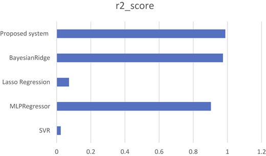
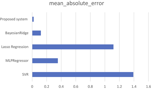
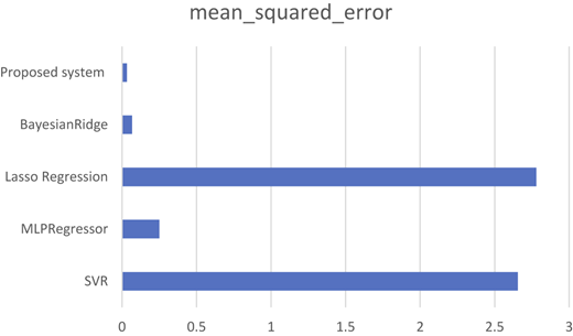
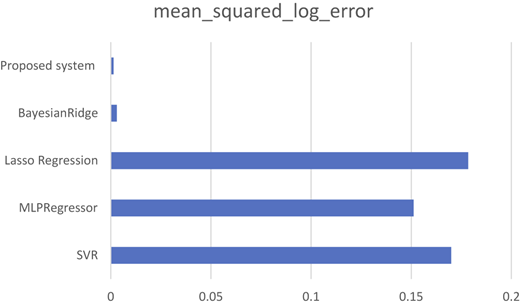
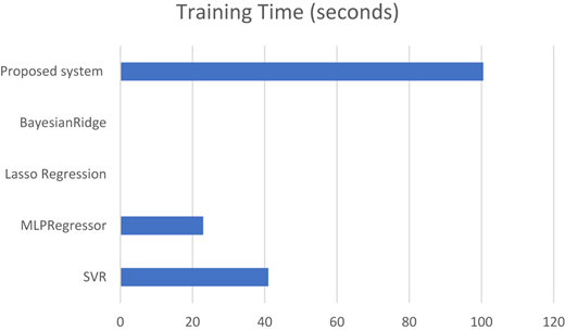
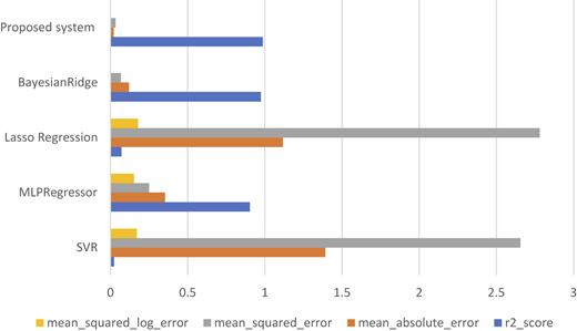
In this section, the results obtained from the proposed system are compared with those of the SVR, MLPRegressor, Lasso Regression, and Bayesian Ridge methods. Table 14 presents the results of these methods across the four evaluated metrics. According to the results shown in this table, the proposed method achieved the highest value in the r2_score metric among all the methods. Since higher values in this metric are more desirable, the proposed method attained the best possible value. For better comparison, the values obtained by different methods for this metric are presented in Figure 3. Figures 4–6 compare the performance of the methods in terms of the mean_absolute_error, mean_squared_error, and mean_squared_log_error metrics, respectively. Since lower values in these metrics are more desirable, the proposed method demonstrated the best performance by achieving the lowest values among all methods (Figure 7).

Figure 8 presents a comparison of the evaluation metrics for the different machine learning models implemented in this study. The bar chart clearly illustrates the performance of each model, allowing for a direct comparison of their predictive error measures. This visual representation underscores the effectiveness of the proposed approach in comparison to other models employed.

One of the issues that can impact all models is the quality and completeness of the data. Incomplete data or the lack of sufficient features can lead to errors in predictions. For example, some features may not have a significant impact on predicting transportation delays but may still be included in the models, which can reduce the accuracy of the model. Another potential source of error is the sensitivity of the model to parameter tuning, where improper settings may affect the overall performance. The use of the Firefly algorithm for feature selection and parameter tuning in the proposed system has likely been one of the key reasons for its superiority over other models. Optimizing parameters and selecting features can help reduce these errors and improve model accuracy.

In this study, we proposed a machine learning-based model for predicting transportation delays in supply chains, leveraging the Firefly algorithm for feature selection and parameter optimization. The results indicated that the model outperformed traditional methods such as Support Vector Regression (SVR) and Multi-layer Perceptron (MLP) in terms of prediction accuracy. The Firefly algorithm's ability to efficiently explore the parameter space and select relevant features likely contributed to the improved performance of the proposed model.

One of the key findings from the experiments was that the model with optimized parameters and relevant features, selected using the Firefly algorithm, achieved significantly better accuracy and reduced errors. This result is in line with the literature, which emphasizes the importance of proper feature selection and parameter tuning in enhancing the performance of predictive models. Overall, the findings suggest that machine learning models, particularly those incorporating optimization techniques like the Firefly algorithm, can significantly improve transportation delay prediction in supply chains. However, further research is required to enhance the model's adaptability and applicability to different scenarios and data environments.

This study contributes to the theoretical landscape of predictive analytics and supply chain management by demonstrating how bio-inspired optimization algorithms, when integrated with machine learning models, can significantly enhance predictive accuracy in operational contexts. While much of the existing literature on transportation delay prediction has focused on applying off-the-shelf machine learning techniques, our findings highlight the theoretical value of embedding intelligent metaheuristics—specifically the Firefly Algorithm—within these models. This hybridization bridges a conceptual gap by linking biologically inspired optimization with practical regression-based forecasting in logistics.

Theoretically, this integration opens new avenues for understanding how dynamic optimization strategies can be tailored to accommodate the non-linear, high-dimensional nature of real-world supply chain data. Rather than treating feature selection and parameter tuning as ancillary preprocessing steps, our approach positions them as core theoretical components of model design. This reframing suggests that optimization is not merely a computational necessity but a central mechanism that shapes the learning capacity of predictive models. As such, it encourages scholars to rethink the role of model architecture from a systems perspective—where optimization, feature relevance, and learning interact in complex, often non-obvious ways.

Furthermore, the study adds to the growing body of work exploring explainable and interpretable machine learning. By using decision tree regression as the foundational learning algorithm, our model maintains a level of transparency often lacking in more complex ensemble or deep learning approaches. The theoretical implication here is that there is still substantial value in interpretable models, particularly when enhanced through intelligent tuning techniques, for domains like supply chain management that demand both accuracy and clarity in decision-making.

Lastly, this research suggests a broader theoretical implication concerning model generalizability. The demonstrated performance of the proposed system, even without reliance on deep learning infrastructure, challenges prevailing assumptions that higher model complexity is always necessary for superior results. Instead, it foregrounds the theoretical promise of lean, hybrid frameworks that leverage algorithmic synergy rather than brute computational force—a perspective that may influence future research in resource-constrained environments.

This study offers a number of takeaways that are directly relevant to people working in logistics and supply chain management. One of the most immediate benefits is the potential for improving day-to-day decision-making. Being able to predict transportation delays more accurately means logistics teams can act earlier—rerouting shipments, informing customers in advance, or making better use of warehouse space while waiting for delayed goods. These are not just technical improvements; they can help reduce customer complaints, missed deadlines, and last-minute firefighting.

Another practical strength of the model lies in its efficiency. Many machine learning tools promise high accuracy, but they often require powerful hardware or cloud-based infrastructure, which smaller companies may not have access to. In contrast, our approach runs well on a standard computer, making it accessible to a wider range of organizations. For practitioners, this means it's actually feasible to implement—not just in theory, but in the real, often resource-limited environments where many logistics decisions are made.

The combination of decision tree regression with the Firefly Algorithm also helps teams better understand what's driving delays. Because the model selects the most important features from the data, companies can learn which variables really matter in their specific context—be it traffic conditions, time of year, or route characteristics. This insight can support more targeted improvements, like choosing different carriers, adjusting delivery schedules, or even redesigning parts of the supply chain.

Lastly, the flexibility of the approach means it can be adapted beyond just one type of delivery or geography. Whether it's road transport in urban areas or shipping goods across borders, the model can be trained with local data to reflect the specific challenges of each context. For supply chain managers, this adaptability is a key strength—it allows them to build smarter, more resilient systems without having to start from scratch each time.

While the proposed system demonstrates promising results in predicting transportation delays, several limitations should be considered when interpreting the findings:

Data Quality and Availability: The accuracy of the proposed model is highly dependent on the quality and completeness of the data used for training and testing. Incomplete, noisy, or inconsistent data may lead to unreliable predictions. Additionally, the model may not generalize well to scenarios where data is scarce or of poor quality.

Feature Selection and Dimensionality: The feature selection process, which is carried out using the Firefly algorithm, plays a crucial role in model performance. However, the quality of the selected features can impact the model's accuracy. If irrelevant or redundant features are selected, it may degrade the model's performance. Moreover, the model's performance may be limited by the dimensionality of the feature space.

Considering these limitations will provide valuable insights into the scope and potential areas of improvement for future research.

The proposed model demonstrates significant potential for generalization beyond the supply chain domain. It can be adapted to maritime, air cargo, or urban delivery scenarios with minimal adjustments, thanks to the flexibility of machine learning algorithms and the optimization techniques used in the Firefly algorithm. However, further adaptation and testing are needed to address the unique challenges, operational dynamics, and data characteristics specific to these domains. In future work, a detailed evaluation of the model's performance in these varied contexts should be conducted to validate its effectiveness and robustness. Additionally, expanding the model to handle real-time data and incorporating more diverse features could improve its predictive accuracy and practical applicability. Furthermore, to exploit the benefits of other machine learning methods, predictions from multiple models can be combined in the future using techniques such as bagging, boosting, or stacking.

In this study, a novel prediction system for forecasting transportation delays was proposed, which combines the Decision Tree Regression method with an optimization algorithm based on the Firefly Algorithm (FFA). The proposed system was evaluated using multiple regression models, including Support Vector Regression (SVR), MLPRegressor, Logistic Regression, and Bayesian Ridge, and compared in terms of key performance metrics.

The results demonstrated that the proposed method significantly outperformed the baseline models across all metrics. Specifically, it achieved the highest r2_score of 0.987, indicating excellent predictive accuracy. Furthermore, the proposed system also showed superior performance in terms of error metrics, achieving the lowest mean_absolute_error (0.021), mean_squared_error (0.033), and mean_squared_log_error (0.001), highlighting its effectiveness in minimizing prediction errors.

The optimization of model parameters through the Firefly Algorithm, combined with feature selection, contributed to enhancing the overall performance of the system. The results suggest that the integration of decision tree regression with a metaheuristic optimization technique like FFA is highly effective for tackling complex regression problems, such as transportation delay prediction. This study provides valuable insights into the potential of hybrid machine learning techniques for solving real-world challenges in logistics and supply chain management.
Al-Saghir
,
R.
(
2022
), “
Predicting delays in the supply chain with the use of machine learning
”,
Master's thesis, York University
,
Toronto
.
Alnahhal
,
M.
,
Ahrens
,
D.
and
Salah
,
B.
(
2021
), “
Dynamic lead-time forecasting using machine learning in a make-to-order supply chain
”,
Applied Sciences
, Vol. 
11
No. 
21
, 10105, doi: .
Amellal
,
A.
,
Amellal
,
I.
,
Seghiouer
,
H.
and
Ech-Charrat
,
M.
(
2023
), “
Improving lead time forecasting and anomaly detection for automotive spare parts with a combined CNN-LSTM approach
”,
Operations and Supply Chain Management: International Journal
, Vol. 
16
No. 
2
, pp. 
265
-
278
, doi: .
Balster
,
A.
,
Hansen
,
O.
,
Friedrich
,
H.
and
Ludwig
,
A.
(
2020
), “
An ETA prediction model for intermodal transport networks based on machine learning
”,
Business and Information Systems Engineering
, Vol. 
62
No. 
5
, pp. 
403
-
416
, doi: .
Bani-Mustafa
,
A.
,
Abuorf
,
S.
,
Al-Jumlah
,
R.
,
Al-Mutair
,
M.
,
Kattan
,
H.
,
Al-Muzaiel
,
H.
,
Al-Kahtani
,
F.
,
Al-Subaie
,
A.
,
Al-Dosari
,
A.
,
Al-Otaibi
,
R.
and
Patwa
,
N.
(
2018
), “
Predicting total shipping and clearance time for Al-Ghanim Sahara transportation
”,
Electronic Journal of Applied Statistical Analysis
, Vol. 
11
No. 
2
, pp.
405
-
426
.
Barros
,
J.
,
Gonçalves
,
J.N.
,
Cortez
,
P.
and
Carvalho
,
M.S.
(
2023
), “
A decision support system based on a multivariate supervised regression strategy for estimating supply lead times
”,
Engineering Applications of Artificial Intelligence
, Vol. 
125
, 106671, doi: .
Daneshvar
,
A.
,
Olfat
,
M.
,
Pourghader Chobar
,
A.
and
Yadegari
,
E.
(
2025
), “
Improving the performance of direct advertising campaigns by applying artificial intelligence techniques
”,
Corporate Communications: An International Journal
. doi: .
Erkmen
,
O.E.
,
Nigiz
,
E.
,
Sari
,
Z.S.
,
Arli
,
H.S.
and
Akay
,
M.F.
(
2022
), “
Delivery time prediction using support vector machine combined withLook-back approach
”,
AINTELIA Science Notes Journal
, Vol. 
1
No. 
1
, pp.
1
-
10
.
Hathikal
,
S.
,
Chung
,
S.H.
and
Karczewski
,
M.
(
2020
), “
Prediction of ocean import shipment lead time using machine learning methods
”,
SN Applied Sciences
, Vol. 
2
No. 
7
, p.
1272
, doi: .
Huang
,
P.
,
Wen
,
C.
,
Fu
,
L.
,
Peng
,
Q.
and
Tang
,
Y.
(
2020
), “
A deep learning approach for multi-attribute data: a study of train delay prediction in railway systems
”,
Information Sciences
, Vol. 
516
, pp. 
234
-
253
, doi: .
Jain
,
A.
(
2018
), “
Responding to shipment delays: the roles of operational flexibility & lead‐time visibility
”,
Decision Sciences
, Vol. 
49
No. 
2
, pp. 
306
-
334
.
Kandula
,
S.
,
Krishnamoorthy
,
S.
and
Roy
,
D.
(
2021
), “
A prescriptive analytics framework for efficient E-commerce order delivery
”,
Decision Support Systems
, Vol. 
147
, 113584, doi: .
Lochbrunner
,
M.
and
Witschel
,
H.F.
(
2022
), “
Combining machine learning with human knowledge for delivery time estimations
”,
Proceedings of the Workshops of the EDBT/ICDT 2022 Joint Conference
,
Edinburgh
.
Mahajan
,
P.C.
,
Kiwelekar
,
A.W.
,
Netak
,
L.D.
and
Ghodake
,
A.B.
(
2022
), “
Predicting expected time of arrival of shipments through multiple linear regression
”,
ICDSMLA 2020: Proceedings of the 2nd International Conference on Data Science, Machine Learning and Applications
,
Springer
,
Singapore
, pp. 
343
-
350
.
Pineda-Jaramillo
,
J.
and
Viti
,
F.
(
2023
), “
Identifying the rail operating features associated to intermodal freight rail operation delays
”,
Transportation Research Part C: Emerging Technologies
, Vol. 
147
, 103993, doi: .
Pineda-Jaramillo
,
J.
,
Bigi
,
F.
,
Bosi
,
T.
,
Viti
,
F.
and
D’ariano
,
A.
(
2023
), “
Short-term arrival delay time prediction in freight rail operations using data-driven models
”,
IEEE Access
, Vol. 
11
, pp. 
46966
-
46978
, doi: .
Polim
,
R.
,
Kumara
,
S.
and
Gomes
,
B.M.
(
2017
), “
Real-time shipment duration prediction
”,
IIE Annual Conference. Proceedings
,
Institute of Industrial and Systems Engineers (IISE)
, pp. 
1607
-
1612
.
Servos
,
N.
,
Liu
,
X.
,
Teucke
,
M.
and
Freitag
,
M.
(
2019
), “
Travel time prediction in a multimodal freight transport relation using machine learning algorithms
”,
Logistics
, Vol. 
4
No. 
1
, p.
1
, doi: .
Shi
,
R.
,
Xu
,
X.
,
Li
,
J.
and
Li
,
Y.
(
2021
), “
Prediction and analysis of train arrival delay based on XGBoost and Bayesian optimization
”,
Applied Soft Computing
, Vol. 
109
, 107538, doi: .
Khiari
,
J.
and
Olaverri-Monreal
,
C.
(
2020
), “
Boosting algorithms for delivery time prediction in transportation logistics
”,
2020 International Conference on Data Mining Workshops (ICDMW)
,
IEEE
, pp. 
251
-
258
.
Published in Modern Supply Chain Research and Applications. Published by Emerald Publishing Limited. This article is published under the Creative Commons Attribution (CC BY 4.0) licence. Anyone may reproduce, distribute, translate and create derivative works of this article (for both commercial and non-commercial purposes), subject to full attribution to the original publication and authors. The full terms of this licence may be seen at Link to the terms of the CC BY 4.0 licence.

Data & Figures

Figure 1
A figure shows S V M, X G Boost, light G B M, research gaps, and optimization with the Firefly algorithm.The figure begins with the text “The models available in the articles reviewed” written on the top left. A downward arrow points the text to a vertical list that contains three text boxes, labeled from top to bottom as “S V M,” “X G Boost,” and “Light G B M.” Between “X G Boost” and “Light G B M,” three horizontally arranged dots are present. A rightward arrow from the “Light G B M” is placed at the bottom. The box in the center labeled “Research Gap” contains three vertically arranged rectangles, labeled from top to bottom as “Lack of parameter optimization,” “Lack of feature selection,” and “The need for more comprehensive models.” A cornered rightward arrow points the center box to a box on the right labeled “Model optimization with the Firefly algorithm,” which contains two rectangles arranged vertically, labeled “Parameter optimization” and “Selection of effective features.”

Positioning of the study within the existing landscape. Source(s): The authors

Figure 1
A figure shows S V M, X G Boost, light G B M, research gaps, and optimization with the Firefly algorithm.The figure begins with the text “The models available in the articles reviewed” written on the top left. A downward arrow points the text to a vertical list that contains three text boxes, labeled from top to bottom as “S V M,” “X G Boost,” and “Light G B M.” Between “X G Boost” and “Light G B M,” three horizontally arranged dots are present. A rightward arrow from the “Light G B M” is placed at the bottom. The box in the center labeled “Research Gap” contains three vertically arranged rectangles, labeled from top to bottom as “Lack of parameter optimization,” “Lack of feature selection,” and “The need for more comprehensive models.” A cornered rightward arrow points the center box to a box on the right labeled “Model optimization with the Firefly algorithm,” which contains two rectangles arranged vertically, labeled “Parameter optimization” and “Selection of effective features.”

Positioning of the study within the existing landscape. Source(s): The authors

Close modal
Figure 2
A flowchart of data preprocessing, feature selection, decision tree modeling, parameter tuning, and evaluation.The flowchart starts at the top with three boxes arranged vertically, connected by downward arrows labeled “Receive data,” followed by “Data preprocessing” and “Data division.” “Data division” splits into two branches: “Test data” on the left and “Training data” on the right. Below “Test data” and “Training data,” three vertical columns with text boxes are shown arranged horizontally. The first column under “Test data,” is a dashed box titled “Feature selection with F A” containing the following vertical sequence of text boxes connected by downward arrow: “Determining parameters and stopping criteria,” “Creating the initial population,” “Objective function calculation,” “The movement of dim fireflies towards brighter fireflies,” “Updating the brightness and position of the fireflies,” “Objective function calculation.” A downward arrow leads to a diamond labeled “Stopping criterion,” which loops back up to the “The movement of dim fireflies towards brighter fireflies” box. A downward arrow from the diamond leads to a textbox outside the dashed rectangle labeled “Reporting the best solution by the algorithm.” The second column in the middle has text boxes in a vertical sequence, labeled from top to bottom as “Building a decision tree model based on selected features,” followed by “Building a decision tree model based on the values set for the parameters,” followed by a solid rectangle containing four vertically arranged boxes “Building a decision tree model,” “Model training,” “Model prediction,” and “Calculating evaluation criteria.” A downward arrow from the top box points to the solid rectangle at the top. A downward arrow from the second box points to the rectangle at the right side. A downward arrow from “Training data” also points to the solid rectangle. A line is shown between the first box, “Building a decision tree model based on selected features,” and both the text boxes with the text “Objective function calculation” in the first section. To the right, the third column is shown with a dashed box titled “Parameters tuning with F A” contains vertical sequence of text boxes connected by downward arrow labeled from top to bottom labeled “Determining parameters and stopping criteria,” “Creating the initial population,” “Objective function calculation,” “The movement of dim fireflies towards brighter fireflies,” “Updating the brightness and position of the fireflies,” “Objective function calculation.” A downward arrow leads to a diamond labeled “Stopping criterion,” which loops back up to the “The movement of dim fireflies towards brighter fireflies” box. A downward arrow from the diamond leads to a textbox outside the dashed rectangle labeled “Reporting the best solution by the algorithm.” A leftward arrow from both the text boxes with the text “Objective function calculation” in the right column points to “Building a decision tree model based on the values set for the parameters” on the middle section. Both reporting boxes connect downward to “Applying the final model to the test data,” followed by “Results and evaluation” at the bottom. A downward arrow from “Test data” points to “Applying the final model to the test data.”

Proposed system for predicting transportation delays. Source(s): The authors

Figure 2
A flowchart of data preprocessing, feature selection, decision tree modeling, parameter tuning, and evaluation.The flowchart starts at the top with three boxes arranged vertically, connected by downward arrows labeled “Receive data,” followed by “Data preprocessing” and “Data division.” “Data division” splits into two branches: “Test data” on the left and “Training data” on the right. Below “Test data” and “Training data,” three vertical columns with text boxes are shown arranged horizontally. The first column under “Test data,” is a dashed box titled “Feature selection with F A” containing the following vertical sequence of text boxes connected by downward arrow: “Determining parameters and stopping criteria,” “Creating the initial population,” “Objective function calculation,” “The movement of dim fireflies towards brighter fireflies,” “Updating the brightness and position of the fireflies,” “Objective function calculation.” A downward arrow leads to a diamond labeled “Stopping criterion,” which loops back up to the “The movement of dim fireflies towards brighter fireflies” box. A downward arrow from the diamond leads to a textbox outside the dashed rectangle labeled “Reporting the best solution by the algorithm.” The second column in the middle has text boxes in a vertical sequence, labeled from top to bottom as “Building a decision tree model based on selected features,” followed by “Building a decision tree model based on the values set for the parameters,” followed by a solid rectangle containing four vertically arranged boxes “Building a decision tree model,” “Model training,” “Model prediction,” and “Calculating evaluation criteria.” A downward arrow from the top box points to the solid rectangle at the top. A downward arrow from the second box points to the rectangle at the right side. A downward arrow from “Training data” also points to the solid rectangle. A line is shown between the first box, “Building a decision tree model based on selected features,” and both the text boxes with the text “Objective function calculation” in the first section. To the right, the third column is shown with a dashed box titled “Parameters tuning with F A” contains vertical sequence of text boxes connected by downward arrow labeled from top to bottom labeled “Determining parameters and stopping criteria,” “Creating the initial population,” “Objective function calculation,” “The movement of dim fireflies towards brighter fireflies,” “Updating the brightness and position of the fireflies,” “Objective function calculation.” A downward arrow leads to a diamond labeled “Stopping criterion,” which loops back up to the “The movement of dim fireflies towards brighter fireflies” box. A downward arrow from the diamond leads to a textbox outside the dashed rectangle labeled “Reporting the best solution by the algorithm.” A leftward arrow from both the text boxes with the text “Objective function calculation” in the right column points to “Building a decision tree model based on the values set for the parameters” on the middle section. Both reporting boxes connect downward to “Applying the final model to the test data,” followed by “Results and evaluation” at the bottom. A downward arrow from “Test data” points to “Applying the final model to the test data.”

Proposed system for predicting transportation delays. Source(s): The authors

Close modal
Figure 3
A horizontal bar chart compares r 2 scores of different regression models, including a proposed system.The horizontal axis is labeled “r 2 underscore score” and ranges from 0.0 to 1.2 in increments of 0.2. The vertical axis shows five models labeled from top to bottom as “Proposed system,” “Bayesian Ridge,” “Lasso Regression,” “M L P Regressor,” and “S V R.” Each model has one horizontal bar. The data from the bars is as follows: Proposed system: 0.9874386149707637. Bayesian Ridge: 0.973760755266179. Lasso Regression: 0.07212224444914517. M L P Regressor: 0.903430709270961. S V R: 0.02396156237326541. Note: All numerical data values are approximated.

Comparison of the results obtained from the proposed system and the baseline methods in the R2_score criterion. Source(s): The authors

Figure 3
A horizontal bar chart compares r 2 scores of different regression models, including a proposed system.The horizontal axis is labeled “r 2 underscore score” and ranges from 0.0 to 1.2 in increments of 0.2. The vertical axis shows five models labeled from top to bottom as “Proposed system,” “Bayesian Ridge,” “Lasso Regression,” “M L P Regressor,” and “S V R.” Each model has one horizontal bar. The data from the bars is as follows: Proposed system: 0.9874386149707637. Bayesian Ridge: 0.973760755266179. Lasso Regression: 0.07212224444914517. M L P Regressor: 0.903430709270961. S V R: 0.02396156237326541. Note: All numerical data values are approximated.

Comparison of the results obtained from the proposed system and the baseline methods in the R2_score criterion. Source(s): The authors

Close modal
Figure 4
A horizontal bar chart compares mean absolute error values of five regression models.The horizontal axis is labeled “mean underscore absolute underscore error” and ranges from 0 to 1.6 in increments of 0.2 units. The vertical axis shows five models labeled from top to bottom as “Proposed system,” “Bayesian Ridge,” “Lasso Regression,” “M L P Regressor,” and “S V R.” Each model has one horizontal bar. The data from the bars is as follows: Proposed system: 0.02104680144004431. Bayesian Ridge: 0.12000069161608086. Lasso Regression: 1.1176959291055109. M L P Regressor: 0.3532405382998605. S V R: 1.3914231007438331. Note: All numerical data values are approximated.

Comparison in the mean_absolute_error criterion. Source(s): The authors

Figure 4
A horizontal bar chart compares mean absolute error values of five regression models.The horizontal axis is labeled “mean underscore absolute underscore error” and ranges from 0 to 1.6 in increments of 0.2 units. The vertical axis shows five models labeled from top to bottom as “Proposed system,” “Bayesian Ridge,” “Lasso Regression,” “M L P Regressor,” and “S V R.” Each model has one horizontal bar. The data from the bars is as follows: Proposed system: 0.02104680144004431. Bayesian Ridge: 0.12000069161608086. Lasso Regression: 1.1176959291055109. M L P Regressor: 0.3532405382998605. S V R: 1.3914231007438331. Note: All numerical data values are approximated.

Comparison in the mean_absolute_error criterion. Source(s): The authors

Close modal
Figure 5
A horizontal bar chart compares the mean squared error values of five regression models.The horizontal axis is labeled “mean underscore squared underscore error” and ranges from 0 to 3 in increments of 0.5 units. The vertical axis shows five models labeled from top to bottom as “Proposed system,” “Bayesian Ridge,” “Lasso Regression,” “M L P Regressor,” and “S V R.” Each model has one horizontal bar. The data from the bars is as follows: Proposed system: 0.033231791747438386. Bayesian Ridge: 0.06803411288368112. Lasso Regression: 2.779839379673221. M L P Regressor: 0.25038853416722306. S V R: 2.6549665293246676. Note: All numerical data values are approximated.

Comparison in the mean_squared_error criterion. Source(s): The authors

Figure 5
A horizontal bar chart compares the mean squared error values of five regression models.The horizontal axis is labeled “mean underscore squared underscore error” and ranges from 0 to 3 in increments of 0.5 units. The vertical axis shows five models labeled from top to bottom as “Proposed system,” “Bayesian Ridge,” “Lasso Regression,” “M L P Regressor,” and “S V R.” Each model has one horizontal bar. The data from the bars is as follows: Proposed system: 0.033231791747438386. Bayesian Ridge: 0.06803411288368112. Lasso Regression: 2.779839379673221. M L P Regressor: 0.25038853416722306. S V R: 2.6549665293246676. Note: All numerical data values are approximated.

Comparison in the mean_squared_error criterion. Source(s): The authors

Close modal
Figure 6
A horizontal bar chart compares the mean squared log error values of five regression models.The horizontal axis is labeled “mean underscore squared underscore log underscore error” and ranges from 0 to 0.2 in increments of 0.05 units. The vertical axis shows five models labeled from top to bottom as “Proposed system,” “Bayesian Ridge,” “Lasso Regression,” “M L P Regressor,” and “S V R.” Each model has one horizontal bar. The data from the bars is as follows: Proposed system: 0.0013806880733000701. Bayesian Ridge: 0.0030741688251750576. Lasso Regression: 0.17843386082033053. M L P Regressor: 0.15123498513411204. S V R: 0.16994458128649434. Note: All numerical data values are approximated.

Comparison in the mean_squared_log_error criterion. Source(s): The authors

Figure 6
A horizontal bar chart compares the mean squared log error values of five regression models.The horizontal axis is labeled “mean underscore squared underscore log underscore error” and ranges from 0 to 0.2 in increments of 0.05 units. The vertical axis shows five models labeled from top to bottom as “Proposed system,” “Bayesian Ridge,” “Lasso Regression,” “M L P Regressor,” and “S V R.” Each model has one horizontal bar. The data from the bars is as follows: Proposed system: 0.0013806880733000701. Bayesian Ridge: 0.0030741688251750576. Lasso Regression: 0.17843386082033053. M L P Regressor: 0.15123498513411204. S V R: 0.16994458128649434. Note: All numerical data values are approximated.

Comparison in the mean_squared_log_error criterion. Source(s): The authors

Close modal
Figure 7
A horizontal bar chart compares the training time of five regression models.The horizontal axis is labeled “Training Time (seconds)” and ranges from 0 to 120 in increments of 20 units. The vertical axis shows five models labeled from top to bottom as follows: “Proposed system,” “Bayesian Ridge,” “Lasso Regression,” “M L P Regressor,” and “S V R.” Each model has one horizontal bar. The data from the bars is as follows: Proposed system: 103.52. Bayesian Ridge: 0.03. Lasso Regression: 0.04. M L P Regressor: 22.92. S V R: 40.97. Note: All numerical data values are approximated.

Comparison in the training time(seconds). Source(s): The authors

Figure 7
A horizontal bar chart compares the training time of five regression models.The horizontal axis is labeled “Training Time (seconds)” and ranges from 0 to 120 in increments of 20 units. The vertical axis shows five models labeled from top to bottom as follows: “Proposed system,” “Bayesian Ridge,” “Lasso Regression,” “M L P Regressor,” and “S V R.” Each model has one horizontal bar. The data from the bars is as follows: Proposed system: 103.52. Bayesian Ridge: 0.03. Lasso Regression: 0.04. M L P Regressor: 22.92. S V R: 40.97. Note: All numerical data values are approximated.

Comparison in the training time(seconds). Source(s): The authors

Close modal
Figure 8
A horizontal grouped bar chart compares five regression methods across 4 evaluation measures.The vertical axis of the grouped horizontal bar graph lists five methods: “Proposed system,” “Bayesian Ridge,” “Lasso Regression,” “M L P Regressor,” and “S V R.” The horizontal axis of the graph represents error and score values. The graph contains four colored horizontal bars for each method, corresponding to the metrics “mean underscore squared underscore log underscore error,” “mean underscore squared underscore error,” “mean underscore absolute underscore error,” and “r 2 underscore score.” The legend at the bottom identifies the color assigned for each error and score values. The data from the graph is as follows: Proposed system: mean underscore squared underscore log underscore error: 0.00138; mean underscore squared underscore error: 0.03323; mean underscore absolute underscore error: 0.02105; r 2 underscore score: 0.98744. Bayesian Ridge: mean underscore squared underscore log underscore error: 0.00307; mean underscore squared underscore error: 0.06803; mean underscore absolute underscore error: 0.12000; r 2 underscore score: 0.97376. Lasso Regression: mean underscore squared underscore log underscore error: 0.17843; mean underscore squared underscore error: 2.77989; mean underscore absolute underscore error: 1.11770; r 2 underscore score: 0.07212. M L P Regressor: mean underscore squared underscore log underscore error: 0.15123; mean underscore squared underscore error: 0.25039; mean underscore absolute underscore error: 0.35324; r 2 underscore score: 0.90343. S V R: mean underscore squared underscore log underscore error: 0.16994; mean underscore squared underscore error: 2.65497; mean underscore absolute underscore error: 1.39142; r 2 underscore score: 0.02396.

Comparison of results in different implemented methods. Source(s): The authors

Figure 8
A horizontal grouped bar chart compares five regression methods across 4 evaluation measures.The vertical axis of the grouped horizontal bar graph lists five methods: “Proposed system,” “Bayesian Ridge,” “Lasso Regression,” “M L P Regressor,” and “S V R.” The horizontal axis of the graph represents error and score values. The graph contains four colored horizontal bars for each method, corresponding to the metrics “mean underscore squared underscore log underscore error,” “mean underscore squared underscore error,” “mean underscore absolute underscore error,” and “r 2 underscore score.” The legend at the bottom identifies the color assigned for each error and score values. The data from the graph is as follows: Proposed system: mean underscore squared underscore log underscore error: 0.00138; mean underscore squared underscore error: 0.03323; mean underscore absolute underscore error: 0.02105; r 2 underscore score: 0.98744. Bayesian Ridge: mean underscore squared underscore log underscore error: 0.00307; mean underscore squared underscore error: 0.06803; mean underscore absolute underscore error: 0.12000; r 2 underscore score: 0.97376. Lasso Regression: mean underscore squared underscore log underscore error: 0.17843; mean underscore squared underscore error: 2.77989; mean underscore absolute underscore error: 1.11770; r 2 underscore score: 0.07212. M L P Regressor: mean underscore squared underscore log underscore error: 0.15123; mean underscore squared underscore error: 0.25039; mean underscore absolute underscore error: 0.35324; r 2 underscore score: 0.90343. S V R: mean underscore squared underscore log underscore error: 0.16994; mean underscore squared underscore error: 2.65497; mean underscore absolute underscore error: 1.39142; r 2 underscore score: 0.02396.

Comparison of results in different implemented methods. Source(s): The authors

Close modal
Table 1

Summary of some of the methods reviewed

ResearchMethodDatasetEvaluation
Servos et al. (2019) Support Vector Regression (SVR)Real-world multi-dimensional container transportation relationship from Germany to the United StatesPrediction accuracy with a mean absolute error of 17 h for delivery time up to 30 days
Erkmen et al. (2022) Support Vector Machine (SVM)Sample dataset obtained from KaggleMean MAE achieved with the backward-looking approach (3.81)
Mahajan et al. (2022) Multiple Regression TechniquesInternal data on shipments stored by a company, and secondly, maritime traffic data89% accuracy
Kandula et al. (2021) Decision Support FrameworkTwo real-world datasets from a major e-commerce platform10.2% savings in delivery costs
Bani-Mustafa et al. (2018) Fixed and Random Multivariate Regression ModelThree years of data from Elghanem Desert transportation (2014–2016)Detection of 38.7% of all changes in delivery time
Alnahhal et al. (2021) Linear Regression and Logistic RegressionReal data from a logistics companyType 1 error with an average value of 0.07
Barros et al. (2023) Random Forest ModelEmpirical data from a large automobile manufacturerAverage reduction of 18%–24% in mean absolute errors
Pineda-Jaramillo et al. (2023) Tuned LightGBMdata from the Luxembourg National Railway Companyaccuracy of 93.8%
Al-Saghir (2022) Logistic RegressionDataco supply chain dataset from Kaggleaccuracy of 75.13%
Shi et al. (2021) combining eXtreme Gradient Boosting (XGBoost) and Bayesian optimization (BOtwo high-speed railway lines in ChinaRMSE of 2.686/1.887
Source(s): The authors
Table 2

Features of the Dataco smart supply chain dataset

FieldDescriptionFieldDescription
TypeType of transaction conductedOrder CountryDestination country of the order
Days for shipping (real)Actual days for shipping the purchased productOrder Customer IdCustomer's order ID
Days for shipment (scheduled)Scheduled days for shipping the purchased productOrder date (DateOrders)Date when the order was placed
Benefit per orderRevenue per orderOrder IdOrder ID
Sales per customerTotal sales per customerOrder Item Cardprod IdProduct ID generated via RFID reader
Delivery StatusDelivery status of the orderOrder Item DiscountDiscount value of the product
Late_delivery_riskCategorical variable indicating if the delivery was late (1) or not (0)Order Item Discount RateDiscount rate for the product
Category IdProduct category IDOrder Item IdProduct ID of the order item
Category NameDescription of the product categoryOrder Item Product PricePrice of the product without discount
Customer CityCity where the customer made the purchaseOrder Item Profit RatioProfit ratio for the order item
Customer CountryCountry where the customer made the purchaseOrder Item QuantityNumber of products in each order
Customer EmailCustomer's email addressSalesSales value
Customer FnameCustomer's first nameOrder Item TotalTotal amount per order
Customer IdCustomer IDOrder Profit Per OrderProfit per order
Customer LnameCustomer's last nameOrder RegionRegion of the world where the order is delivered
Customer PasswordCustomer's masked keyOrder StateState/Region where the order is delivered
Customer SegmentCustomer types: Consumer, Corporate, Home OfficeOrder StatusOrder status
Customer StateState of the store where the purchase was madeProduct Card IdProduct card ID
Customer StreetStreet of the store where the purchase was madeProduct Category IdProduct category ID
Customer ZipcodeCustomer's postal codeProduct DescriptionDescription of the product
Department IdStore department IDProduct ImageLink to view and purchase the product
Department NameName of the store departmentProduct NameName of the product
LatitudeLatitude of the store locationProduct PriceProduct price
LongitudeLongitude of the store locationProduct StatusProduct stock status
MarketMarket location for order deliveryShipping date (DateOrders)Exact date and time of shipment
Order CityDestination city of the orderShipping ModeShipping modes
Source(s): The authors
Table 3

Dataset split for training and testing

SubsetNumber of records (10%)Percentage
Training Set14,44180%
Testing Set3,61020%
Total18,051100%
Source(s): The authors
Table 4

Set parameter values for SVR method

ParameterValueParameterValueParameterValue
kernel“rbf”degree3gamma“scale”
coef00.0tol0.001C1.0
epsilon0.2shrinkingTruecache_size200
verboseFalse    
Source(s): The authors
Table 5

Results of SVR implementation and testing

MetricObtained value
r2_score0.02396156237326541
mean_absolute_error1.3914231007438331
mean_squared_error2.6549665293246676
mean_squared_log_error0.16994458128649434
Source(s): The authors
Table 6

Set parameter values for MLPRegressor method

ParameterValueParameterValueParameterValue
hidden_layer_sizes100activation“relu”solver“adam”
alpha0.0001batch_size“auto”learning_rate“constant”
learning_rate_init0.001power_t0.5max_iter200
epsilon1e−08n_iter_no_change10random_state1
Source(s): The authors
Table 7

Results of MLPRegressor implementation and testing

MetricObtained value
r2_score0.903430709270961
mean_absolute_error0.3532405382998605
mean_squared_error0.25038853416722306
mean_squared_log_error0.15123498513411204
Source(s): The authors
Table 8

Set parameter values for Lasso regression method

ParameterValue
alpha0.1
fit_interceptTrue
max_iter1,000
precomputeFalse
Source(s): The authors
Table 9

Results of Lasso regression implementation and testing

MetricObtained value
r2_score0.7296480386420201
mean_absolute_error0.6159400265322427
mean_squared_error0.695317345242548
mean_squared_log_error0.05974608146057183
Source(s): The authors
Table 10

Set parameter values for Bayesian Ridge method

ParameterValueParameterValueParameterValue
max_iter300tol0.001alpha_11e−06
alpha_21e−06lambda_11e −06lambda_21e−06
alpha_initNonelambda_initNonecompute_scoreFalse
fit_interceptTruecopy_XTrueVerboseFalse
Source(s): The authors
Table 11

Results of Bayesian Ridge implementation and testing

MetricObtained value
r2_score0.973760755266179
mean_absolute_error0.12000069161608086
mean_squared_error0.06803411288368112
mean_squared_log_error0.0030741688251750576
Source(s): The authors
Table 12

Set parameter values for the proposed method

ParameterValueParameterValueParameterValue
Decision tree parameters 
Criterion“squared_error”Splitter“best”max_depthNone
min_samples_split2min_samples_leaf1min_weight_fraction_leaf0.0
max_featuresNonemin_impurity_decrease0.0ccp_alpha0.0
Firefly parameters
alpha1.0gamma0.5MaxGeneration100
beta01.0population size100  
Source(s): The authors
Table 13

Results of proposed method implementation and testing

MetricObtained value
r2_score0.9874386149707637
mean_absolute_error0.02104680144004431
mean_squared_error0.033231791747438386
mean_squared_log_error0.0013806880733000701
Source(s): The authors
Table 14

Comparison of results from the proposed system and base methods

MetricSVRMLPRegressorLasso regressionBayesianRidgeProposed system
r2_score0.023961562373265410.9034307092709610.072122244449145170.9737607552661790.9874386149707637
mean_absolute_error1.39142310074383310.35324053829986051.11769592910551090.120000691616080860.02104680144004431
mean_squared_error2.65496652932466760.250388534167223062.7798393796732210.068034112883681120.033231791747438386
mean_squared_log_error0.169944581286494340.151234985134112040.178433860820330530.00307416882517505760.0013806880733000701
Training Time (seconds)40.9722.920.040.03103.52
Source(s): The authors

Supplements

References

Al-Saghir
,
R.
(
2022
), “
Predicting delays in the supply chain with the use of machine learning
”,
Master's thesis, York University
,
Toronto
.
Alnahhal
,
M.
,
Ahrens
,
D.
and
Salah
,
B.
(
2021
), “
Dynamic lead-time forecasting using machine learning in a make-to-order supply chain
”,
Applied Sciences
, Vol. 
11
No. 
21
, 10105, doi: .
Amellal
,
A.
,
Amellal
,
I.
,
Seghiouer
,
H.
and
Ech-Charrat
,
M.
(
2023
), “
Improving lead time forecasting and anomaly detection for automotive spare parts with a combined CNN-LSTM approach
”,
Operations and Supply Chain Management: International Journal
, Vol. 
16
No. 
2
, pp. 
265
-
278
, doi: .
Balster
,
A.
,
Hansen
,
O.
,
Friedrich
,
H.
and
Ludwig
,
A.
(
2020
), “
An ETA prediction model for intermodal transport networks based on machine learning
”,
Business and Information Systems Engineering
, Vol. 
62
No. 
5
, pp. 
403
-
416
, doi: .
Bani-Mustafa
,
A.
,
Abuorf
,
S.
,
Al-Jumlah
,
R.
,
Al-Mutair
,
M.
,
Kattan
,
H.
,
Al-Muzaiel
,
H.
,
Al-Kahtani
,
F.
,
Al-Subaie
,
A.
,
Al-Dosari
,
A.
,
Al-Otaibi
,
R.
and
Patwa
,
N.
(
2018
), “
Predicting total shipping and clearance time for Al-Ghanim Sahara transportation
”,
Electronic Journal of Applied Statistical Analysis
, Vol. 
11
No. 
2
, pp.
405
-
426
.
Barros
,
J.
,
Gonçalves
,
J.N.
,
Cortez
,
P.
and
Carvalho
,
M.S.
(
2023
), “
A decision support system based on a multivariate supervised regression strategy for estimating supply lead times
”,
Engineering Applications of Artificial Intelligence
, Vol. 
125
, 106671, doi: .
Daneshvar
,
A.
,
Olfat
,
M.
,
Pourghader Chobar
,
A.
and
Yadegari
,
E.
(
2025
), “
Improving the performance of direct advertising campaigns by applying artificial intelligence techniques
”,
Corporate Communications: An International Journal
. doi: .
Erkmen
,
O.E.
,
Nigiz
,
E.
,
Sari
,
Z.S.
,
Arli
,
H.S.
and
Akay
,
M.F.
(
2022
), “
Delivery time prediction using support vector machine combined withLook-back approach
”,
AINTELIA Science Notes Journal
, Vol. 
1
No. 
1
, pp.
1
-
10
.
Hathikal
,
S.
,
Chung
,
S.H.
and
Karczewski
,
M.
(
2020
), “
Prediction of ocean import shipment lead time using machine learning methods
”,
SN Applied Sciences
, Vol. 
2
No. 
7
, p.
1272
, doi: .
Huang
,
P.
,
Wen
,
C.
,
Fu
,
L.
,
Peng
,
Q.
and
Tang
,
Y.
(
2020
), “
A deep learning approach for multi-attribute data: a study of train delay prediction in railway systems
”,
Information Sciences
, Vol. 
516
, pp. 
234
-
253
, doi: .
Jain
,
A.
(
2018
), “
Responding to shipment delays: the roles of operational flexibility & lead‐time visibility
”,
Decision Sciences
, Vol. 
49
No. 
2
, pp. 
306
-
334
.
Kandula
,
S.
,
Krishnamoorthy
,
S.
and
Roy
,
D.
(
2021
), “
A prescriptive analytics framework for efficient E-commerce order delivery
”,
Decision Support Systems
, Vol. 
147
, 113584, doi: .
Lochbrunner
,
M.
and
Witschel
,
H.F.
(
2022
), “
Combining machine learning with human knowledge for delivery time estimations
”,
Proceedings of the Workshops of the EDBT/ICDT 2022 Joint Conference
,
Edinburgh
.
Mahajan
,
P.C.
,
Kiwelekar
,
A.W.
,
Netak
,
L.D.
and
Ghodake
,
A.B.
(
2022
), “
Predicting expected time of arrival of shipments through multiple linear regression
”,
ICDSMLA 2020: Proceedings of the 2nd International Conference on Data Science, Machine Learning and Applications
,
Springer
,
Singapore
, pp. 
343
-
350
.
Pineda-Jaramillo
,
J.
and
Viti
,
F.
(
2023
), “
Identifying the rail operating features associated to intermodal freight rail operation delays
”,
Transportation Research Part C: Emerging Technologies
, Vol. 
147
, 103993, doi: .
Pineda-Jaramillo
,
J.
,
Bigi
,
F.
,
Bosi
,
T.
,
Viti
,
F.
and
D’ariano
,
A.
(
2023
), “
Short-term arrival delay time prediction in freight rail operations using data-driven models
”,
IEEE Access
, Vol. 
11
, pp. 
46966
-
46978
, doi: .
Polim
,
R.
,
Kumara
,
S.
and
Gomes
,
B.M.
(
2017
), “
Real-time shipment duration prediction
”,
IIE Annual Conference. Proceedings
,
Institute of Industrial and Systems Engineers (IISE)
, pp. 
1607
-
1612
.
Servos
,
N.
,
Liu
,
X.
,
Teucke
,
M.
and
Freitag
,
M.
(
2019
), “
Travel time prediction in a multimodal freight transport relation using machine learning algorithms
”,
Logistics
, Vol. 
4
No. 
1
, p.
1
, doi: .
Shi
,
R.
,
Xu
,
X.
,
Li
,
J.
and
Li
,
Y.
(
2021
), “
Prediction and analysis of train arrival delay based on XGBoost and Bayesian optimization
”,
Applied Soft Computing
, Vol. 
109
, 107538, doi: .
Khiari
,
J.
and
Olaverri-Monreal
,
C.
(
2020
), “
Boosting algorithms for delivery time prediction in transportation logistics
”,
2020 International Conference on Data Mining Workshops (ICDMW)
,
IEEE
, pp. 
251
-
258
.

Languages

or Create an Account

Close Modal
Close Modal