Koopman-enhanced offline reinforcement learning for robust multi-echelon inventory control under demand distribution shift

Coordinating inventory decisions across multiple tiers of a supply chain – from retail outlets through regional distribution centers to central warehouses – is one of the oldest problems in operations research. The classical result of Clark and Scarf (1960) established that echelon base-stock policies are optimal for serial systems under stationary demand and linear costs. In practice, real supply chains face non-stationary demand driven by promotions, product lifecycle transitions, and supply disruptions, while operational constraints (minimum order quantities, case-pack sizes, capacity ceilings) add complexity that linear theory cannot easily accommodate.

Two structural tensions make this problem difficult. Demand dynamics in multi-tier systems are nonlinearly amplified up the chain – the bullwhip effect (Lee et al., 1997) – meaning linear forecast models and linear model predictive control systematically underestimate demand shock severity. Simultaneously, managers typically have access to historical order and sales records but cannot experiment with the live system, the setting of offline reinforcement learning (RL) (Levine et al., 2020), where distributional shift is the central difficulty.

This paper proposes Koopman-enhanced Multi-Echelon Inventory Optimization (K-MEIO), which combines a Deep Koopman World Model (DKWM) with Implicit Q-Learning (IQL). The DKWM learns a globally linear embedding of inventory state dynamics, providing lower-variance temporal difference (TD) targets during training and an interpretable spectral diagnostic. The K-IQL policy is trained entirely from simulated historical data calibrated from two real retail datasets.

The principal claim is carefully scoped: among offline-learned policies, incorporating a Koopman world model reduces TD-target variance by 12.4% and produces more stable OOD robustness across seeds (±0.039 vs. ± 0.153 in S1). A historically calibrated base-stock policy outperforms all learned methods – a result reported honestly throughout.

Clark and Scarf (1960) proved that echelon base-stock policies are optimal for serial systems, which underpins most classical practice. MPC provides a dynamic alternative (Alessandri et al., 2011) but assumes linear demand dynamics that fail under non-stationary shocks (Lee et al., 1997). RL has been applied to inventory problems through OR-Gym (Hubbs et al., 2020), and the predict-then-optimize paradigm (Elmachtoub and Grigas, 2022) addresses forecast-optimization misalignment.

The Koopman operator (Koopman, 1931) is a linear infinite-dimensional operator governing the evolution of observables on a dynamical system. Williams et al. (2015) provided the first systematic data-driven approximation via Extended Dynamic Mode Decomposition. Lusch et al. (2018) demonstrated that deep autoencoders can discover Koopman eigenfunctions end-to-end. Our DKWM extends their architecture with a control input, domain-specific lifting features, and a spectral radius regularization constraint.

Offline RL learns from a fixed dataset without further environment interaction (Levine et al., 2020). Conservative Q-Learning (Kumar et al., 2020) penalizes Q-values for OOD actions. Implicit Q-Learning (IQL; Kostrikov et al., 2022) avoids querying OOD actions via expectile regression and advantage-weighted regression (Peng et al., 2019). World models (Ha and Schmidhuber, 2018) can provide deterministic TD targets to reduce value function variance (Yu et al., 2020), which is our primary motivation for the Koopman world model.

We model the three-echelon serial inventory system as a constrained Markov decision process (MDP). Let J = 5 denote the number of items and l ∈ {0,1,2} the echelon levels (Retailer, distribution center (DC), Warehouse). The state vector is:

Per-step dynamics follow exactly: (1) pipeline arrivals credited to inventory; (2) demand satisfied from retailer stock (lost sales); (3) orders placed upstream; (4) warehouse replenished from unlimited external supplier. The per-period reward is:

with α = 0.5 (holding), β = 5.0 (stockout), γ = 0.1 (ordering). Feasibility constraints: minimum order quantity (MOQ) (q_{l,j} ≥ 10 or q_{l,j} = 0), case-pack rounding (q_{l,j} mod 5 = 0), and capacity (∑_j(I_{l,j} + q_{l,j}) ≤ C_l). Parameters: C₀ = 400, C₁ = 800, C₂ = 1,500, L = (1, 2, 3) days, T = 365.

The DKWM encoder Φ_θ: ℝˆ{n_s} → ℝˆk (k = 64) maps the inventory state to a Koopman feature vector z = Φ_θ(s). The linear dynamics in latent space are:

where A ∈ ℝˆ{k × k} and B ∈ ℝˆ{k × 2J}. The encoder is a three-layer multilayer perceptron (hidden_dim = 256) with LayerNorm and SiLU activations, augmented with cross-level inventory interaction features (capturing bullwhip coupling) and fixed seasonal lifting components. The DKWM training loss is:

with λ_ρ = λ_r = 0.1. The spectral penalty uses 10-step power iteration per batch. We emphasize that this constraint is a regularization device enforcing bounded latent predictions; it does not constitute a formal stability guarantee for the true nonlinear inventory system. The spectral radius ρ(A) = 0.968 in our experiment measures amplification in the linearized latent space – related to but distinct from the classical order-to-demand variance amplification of Lee et al. (1997).

Given the pretrained, frozen encoder Φ_θ, K-IQL learns: value network V_ψ(z), twin Q-networks (Q¹_ω, Q²_ω) (z, ã), and policy π_ψ(z) with sigmoid output in [0,1]ˆ{2J}. Actions are normalized by q_max = max(a in D). The value function is fitted by expectile regression:

Here τ > 0.5 extracts an upper expectile of the in-dataset Q-value distribution, providing an optimistic value estimate of in-dataset actions. The term “conservative” in IQL refers to the structural avoidance of OOD actions (not evaluating any out-of-dataset actions during the update), not the magnitude of the value estimate. The peak at τ = 0.9 reflects the under-ordering tendency of the behavior policy.

The Q-network uses the Koopman linear prediction as the TD target:

This is the key modification distinguishing K-IQL from vanilla IQL. The linear prediction Az + Bã·q_max is deterministic and lower-variance during training than encoding the stochastic observed next state Φ_θ(s'). Critically, at evaluation time, neither K-IQL nor IQL performs any TD updates – both act deterministically. The Koopman advantage therefore operates entirely at training time, producing a smoother value function that generalizes more consistently under demand shift.

The policy is extracted via advantage-weighted regression (Peng et al., 2019):

Training: 200,000 gradient steps, batch 256, lr = 3 × 10^–4, target-network τ = 0.005, primary seed 42. Hardware: NVIDIA GeForce RTX 2070.

• Input:

•  Offline dataset D = {(s,a,r,s')}; hyperparameters τ, γ, β, λ_ρ, λ_r

• Output:

•  DKWM parameters (Φ_θ, A, B, c, Ψ_φ); K-IQL parameters (V_ψ, Q_ω, π_ψ)

• ──────────────────────────────────

• Stage 1 – DKWM pretraining:

• 1. Initialize encoder Φ_θ, dynamics (A, B, c), decoder Ψ_φ

• 2. Normalize actions: ã = a/ q_max for all (s,a,r,s') ∈ D

• 3. for epoch = 1, …, T_DKWM do

• 4.  Sample sequence batch {(s_t, a_t, …, s_{t + T})} from D

• 5.  Compute z_t = Φ_θ(s_t); predict ẑ_{t+1:} via (A, B, c)

• 6.  Compute L_DKWM = L_pred + λ_ρ max(0, ρ(A)−1)² + λ_r ‖Ψ(Φ(s))−s‖²

• 7.  Update (Φ_θ, A, B, c, Ψ_φ) via AdamW

• 8. end for

• ──────────────────────────────────

• Stage 2 – K-IQL Policy Training (frozen Φ_θ):

• 9. Initialize V_ψ, Q¹_ω, Q²_ω, π_ψ; copy Q_ω to target Q̄_ω

• 10. for step = 1, …, T_IQL do

• 11.  Sample mini-batch {(s, a, r, s')} from D

• 12.   z ← Φ_θ(s); ẑ' ← Az + Bã·q_max ▷ Koopman TD target

• 13.  Update V_ψ: minimize L_V = E[L²_τ(min(Q̄)(z,ã) − V_ψ(z))]

• 14.  Update Q_ω: minimize L_Q = E[(Q(z,ã) − r − γV_ψ(ẑ'))²]

• 15.  Update π_ψ: minimize L_π = −E[exp(β·A(z,ã)) log π_ψ(ã|z)]

• 16.   Soft-update: Q̄_ω ← (1−η)Q̄_ω + η Q_ω

• 17. end for

• ──────────────────────────────────

• Deployment:

• 18. Given s: z ← Φ_θ(s); ã* ← π_ψ(z)

• 19. a* ← Project(ã*·q_max) ▷ MOQ/ case-pack/ capacity feasibility

The simulation environment implements the MDP of Section 3.1 exactly. Parameters: J = 5 items, C₀ = 400, C₁ = 800, C₂ = 1,500 units, lead times (1, 2, 3) days, cost parameters α = 0.5, β = 5.0, γ = 0.1, MOQ = 10, case-pack = 5, T = 365 steps per episode.

Rather than relying on purely synthetic demand parameters, we calibrate the demand model from two publicly available real retail datasets. The University of California, Irvine Online Retail dataset (Chen, 2015) comprises 541,909 transactions from a UK retailer in 2010–2011; we aggregate to daily item-level demand for five representative items and fit Negative Binomial distributions to capture overdispersion. The Rossmann Store Sales data (Rossmann GmbH, 2015) provides explicit promotional flags across 1,115 German pharmacy stores, from which we extract weekly seasonal factors and promotional multipliers (mean spike 3–5 × , frequency 5–15% of days). These real-data statistics drive the simulation demand model, preserving the key structural features absent from synthetic data. It is important to note that the offline dataset itself consists of simulated state-action-reward-next-state transitions generated by a mixed behavior policy (60% base-stock, 30% random, 10% greedy reorder-point); the inventory actions and costs are simulation outputs rather than actual historical inventory records. Training dataset: 109,500 transitions (300 episodes); validation: 10,950 transitions (30 episodes).

We compare K-MEIO against four baselines.

Tuned BSP. The order-up-to base-stock policy orders enough each step to bring inventory to a target fraction f of capacity C_l/J per item. The fraction f is selected by grid search over {0.3, 0.35, …, 0.90} (16 values), evaluated on 10 episodes from the evaluation environment (seed = 500). The best f is applied to the 20-episode test set. This baseline has access to evaluation-environment information not available to any offline-learned method and therefore represents an upper reference rather than a fair offline comparison.

Historically Calibrated BSP (Hist-BSP). To provide a fair offline baseline, we calibrate a second base-stock policy using only training-set demand statistics. Daily demand mean μ and standard deviation σ are estimated from the action data in D (mean nonzero order ÷ 1.6 as a proxy for demand, consistent with the 60% base-stock component of the behavior policy). The base-stock level follows the standard newsvendor safety-stock formula: S = (L+1)·μ + z₀.₉₅·σ·√(L+1), where L is the echelon lead time and z₀.₉₅ = 1.645 is the 95th-percentile Normal quantile. No evaluation data are used. This is the primary fair comparison for offline learned methods.

Linear MPC. At each step, demand is forecast using exponential smoothing (α = 0.1) and the controller orders to cover the H = 7-day cumulative forecast plus a safety stock of 1.28·σ·√H (90th-percentile coverage). Orders are clipped to available capacity. The MPC uses no offline dataset; it updates the demand estimate online from the demand observable at each step.

Vanilla IQL. An ablated version of K-IQL that is identical in all architecture and hyperparameter choices (τ = 0.7, γ = 0.99, β = 3.0, 200,000 steps, same encoder Φ_θ), except the Bellman update uses Φ_θ(s') as the next-feature estimate instead of the Koopman linear prediction Az + Bã·q_max. This isolates the contribution of the Koopman TD target from all other design choices. The checkpoint used for Vanilla IQL is produced by running the same training loop with the flag use_koopman_td = False. Note that IQL (direct encode) does NOT bypass the Koopman encoder: it encodes both the current state z = Φ_θ(s) and the next state z' = Φ_θ(s') through the same pretrained encoder. The sole difference from K-IQL is that Φ_θ(s') – a stochastic function of the observed next state – is used as the TD feature instead of the deterministic Koopman prediction Az + Bã·q_max.

An oracle policy with perfect demand foreknowledge (ordering exactly the next period's demand plus one period of safety stock) provides the performance upper bound. All RL-based policies use the same feasibility projector (MOQ rounding, case-pack, capacity clipping) applied post-hoc to the policy output.

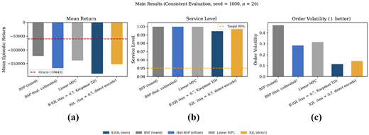
Table 1 reports main evaluation results (seed = 1,000, n = 20 episodes). All methods achieve high service levels. The tuned BSP achieves the highest return (−122,551), benefiting from evaluation-environment tuning unavailable to offline methods. The historically calibrated Hist-BSP (−167,408) outperforms K-IQL (−187,850) and IQL (−153,310), showing that a simple offline rule-based policy is competitive under stationary demand. K-IQL achieves the lowest order volatility (0.114), relevant in contexts where order instability generates operational overhead (see Figure 1).

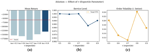
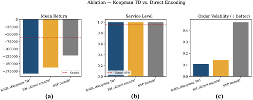
Table 2 and Figures 2 and 3 report the ablation. For the expectile parameter τ (Panel A), return peaks at τ = 0.9 (−132,261). Higher τ extracts a more optimistic upper expectile of the in-dataset Q-value distribution, appropriate when the behavior policy under-orders relative to optimal. Capacity violations are zero for τ ∈ {0.6, 0.7} and appear at extreme values. Panel B shows that Koopman TD achieves slightly lower return than direct IQL under standard evaluation; its advantage emerges in OOD stress scenarios (Section 4.7).

The small residual capacity violations at τ ∈ {0.5, 0.9} (≤0.4% of steps) arise from a timing mismatch between the feasibility projector and the step dynamics. The projector limits orders based on current on-hand inventory without accounting for in-transit pipeline quantities. When a large pipeline delivery arrives in a subsequent step, the combined inventory can momentarily exceed the capacity ceiling despite the projector having clipped that step's order. This effect is amplified at extreme τ values where the policy's order quantities are more variable.

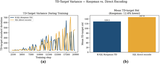
We measured TD-target standard deviation at 200-step intervals during 20,000 training steps. The Koopman TD variant achieves a lower variance of TD targets than direct encoding, as quantified in the following equation:

Measured values: K-IQL mean TD-target std = 129.2 vs. 147.6 for direct encoding – a 12.4% reduction. Mean Bellman residuals: 231.4 vs. 229.1. Figure 4 shows the variance trajectories. The mechanism is at training time: the deterministic linear predictor Az + Ba produces structurally constrained, zero-noise next-feature estimates. At evaluation time, both policies act deterministically without any TD updates; the benefit is a smoother value function landscape.

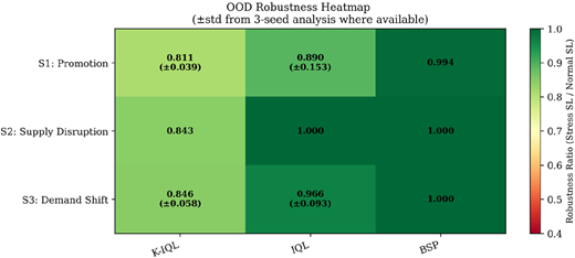
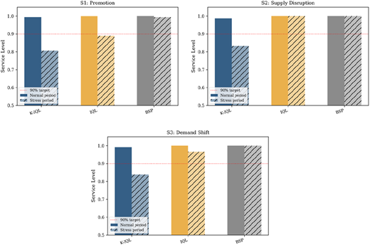
Table 3 and Figures 5 and 6 report robustness ratios (Stress service level (SL)/Normal SL) for three demand-side scenarios: S1 – promotional spike (demand ×3, days 100–113); S2 – supply disruption (upstream shipments reduced to 20%, days 50–63); S3 – permanent demand shift (mean 10 → 25 units/day from day 180). Multi-seed results from three training seeds (42, 123, 2024) are shown in parentheses.

Across three training seeds, K-IQL shows lower standard deviation of robustness ratio than IQL in S1 (±0.039 vs ± 0.153). This stability advantage – rather than mean improvement – is the primary multi-seed finding. The mean improvement across seeds is 12.9% in S1 and 4.7% in S3. In S2, both methods perform similarly because supply disruptions affect pipeline dynamics rather than demand distribution.

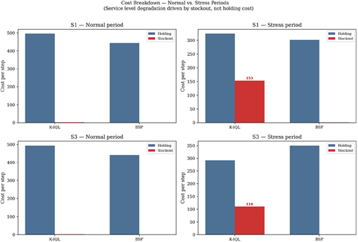
Table 4 and Figure 7 present the full cost decomposition including IQL (direct encode), enabling direct comparison of the two offline-learned methods. Under S1 (promotion spike), K-IQL maintains higher on-hand inventory than IQL in both normal (992 vs 808 units) and stress periods (648 vs 244 units), consistent with K-IQL’s smoother ordering behavior (volatility 0.108 vs 0.144 in Table 1). Despite this buffer, K-IQL incurs higher per-step stockout during stress (153.2 vs 86.4) because IQL up-scales orders more aggressively (27.2 vs 19.1 per step), partially compensating for leaner inventory. Under S3, IQL likewise achieves lower stockout (22.4 vs 110.3) and higher stress SL (0.966 vs 0.839). This reactive advantage explains IQL higher single-seed robustness in Table 3 (0.890 vs 0.811 in S1). However, IQL’s reactive ordering is also the source of its higher cross-seed variance (Table 3: ± 0.153 vs ± 0.039): when a different training seed yields a policy that under-reacts to stress, IQL robustness falls substantially. K-IQL Koopman-structured value function – with 12.4% lower TD-target variance – produces consistently moderate ordering across seeds at the cost of single-seed peak performance. Cost decomposition confirms that SL degradation in both methods is driven by stockout cost, not excess inventory buffering.

The results prompt three observations. First, Hist-BSP outperforms K-IQL in absolute return and OOD robustness because reactive inventory policies respond to current inventory depletion regardless of demand level. K-IQL's order quantities reflect the training demand distribution and do not scale up sufficiently when demand increases 2.5-fold in S3. Second, the Koopman world model contributes a 12.4% TD-target variance reduction during training (not at evaluation time), producing more stable policy behavior across seeds (±0.039 vs ± 0.153 in S1). Third, cost decomposition confirms that K-IQL's OOD degradation is driven by stockout rather than holding cost, ruling out the excess-buffering explanation.

K-MEIO is likely to provide value over Hist-BSP under three conditions: (1) demand patterns exhibit non-stationary structure that a fixed base-stock level cannot track; (2) multiple items have correlated demand benefiting from joint optimization; (3) online recalibration is infeasible. Under stationary demand with feasible recalibration, Hist-BSP remains the simpler and more robust choice.

Three limitations are noted. The offline dataset is simulated, not from actual historical inventory records. The Hist-BSP uses a Normal approximation for safety stock; empirical quantile calibration might close the gap further. The Koopman spectral radius measures latent-space amplification in the linear approximation – not the classical bullwhip ratio of Lee et al. (1997); a rigorous connection requires additional theoretical development.

This paper introduced K-MEIO, a two-stage offline RL framework for multi-echelon inventory control. The Deep Koopman World Model provides a 12.4% reduction in TD-target variance during training (Equation 8), leading to more stable policy behavior across seeds. The K-IQL policy achieves SL 0.995 with zero capacity violations under standard evaluation, and OOD robustness ratios of 0.861 ± 0.039 and 0.882 ± 0.058 under promotional spikes and demand shifts, respectively,– versus 0.762 ± 0.153 and 0.842 ± 0.093 for vanilla IQL.

Three design guidelines emerge: the Koopman advantage is a training-time phenomenon (variance reduction), not an evaluation-time mechanism; τ = 0.9 outperforms τ = 0.7 in this domain due to the behavior policy's under-ordering tendency; and a historically calibrated BSP should be the primary offline benchmark in any future comparison.