Heterogeneous evolution of family firm efficiency

We develop a dynamic family management model to explain why family firm efficiency varies between firms and across time. We hypothesize that family firms experiencing efficiency shortfalls adapt with two tools: (1) family presence in top management; and (2) executive compensation. We show that both tools are important. Greater family presence decreases efficiency, while higher compensation enhances efficiency. Our work has implications for research and practice.

We study family firm heterogeneity over time, in particular, heterogeneity of efficiency. Efficiency is a flexible measure of family firm performance that assesses how close a company is to its best outcome. The dynamics of family firm heterogeneity are important academically, because scholars need to understand how our theoretical models perform when temporal events such as succession, intergenerational relations, and marriage are included. Dynamic heterogeneity is also important from a practical perspective, as family businesses require guidance on what tools best improve performance in the face of succession and other time-related events.

We join an ongoing conversation about time and heterogeneity in family firms. De Massis et al. (2014) formalize a model of family firm proactiveness over time. They conclude that proactiveness is S-shaped, and affected by the dispersion of managerial control among family members. Evert et al. (2016) point out that time is “a key component in numerous family business phenomena and should be included in more empirical analysis, …enabling researchers to address novel … research questions” (p. 31). Madison et al. (2016) indicate that in order to advance research, it is essential to understand the dynamic relationship between governance and behavior, and to examine firm-level outcomes (pp. 84–85). Dyer (2018) underscores the importance of connecting family heterogeneity and firm performance, and of accounting for family experiences over time (pp. 246–247). Kotlar et al. (2020) show that family ownership drives dynamic heterogeneity in absorptive capacity. Our work builds mainly on De Massis et al. (2014) and Kotlar et al. (2020), which we extend by introducing a microfounded measure of family firm performance – technical efficiency. Moreover, we emphasize the dynamic relation between executive compensation and a specific aspect of family control, namely, family involvement in the management team. A unique theoretical contribution is that the combination of compensation and family involvement strongly drives dynamic family firm efficiency.

While the above research has made tantalizing inroads in the question of family firm heterogeneity over time, there is still much to do. We focus on two research gaps. First, it is important to have a theoretical framework that highlights primary drivers of dynamic heterogeneity in family firm performance. Is heterogeneity just attributable to the effect of time on family relations and governance, or do other channels matter? Ex ante, it is difficult to think of a single variable to answer this question. Therefore it is crucial to build a new dynamic theory to guide our reasoning. Second, it is valuable to develop longitudinal datasets and empirical techniques, in order to test and refine the theory. For concreteness we focus on the specific performance measure of technical efficiency: a firm's ability to maximize production for a given level of inputs (Kumbhakar and Lovell, 2000, Chapter 2). Efficiency is therefore the ratio of existing production to maximum production ^[1].

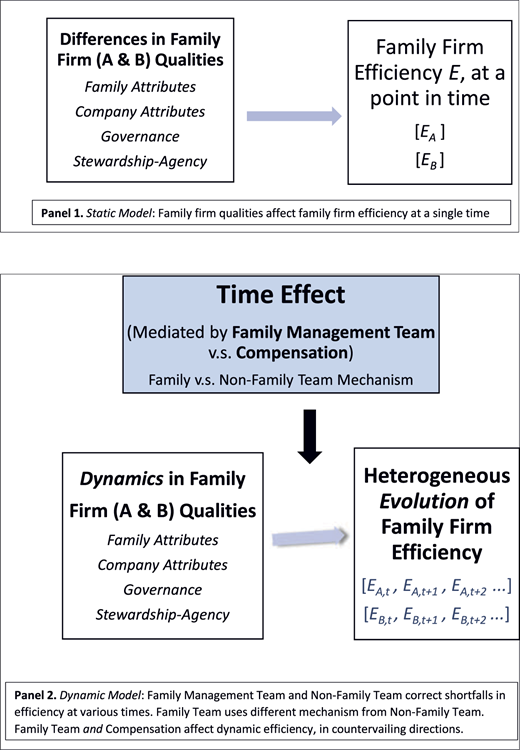
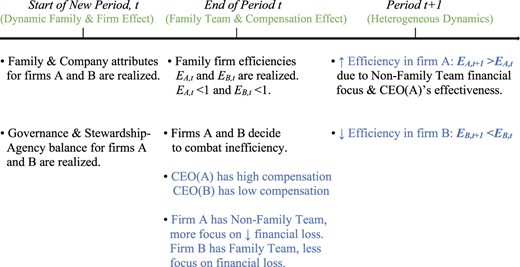
We proceed in two steps. We first offer a theory of dynamic heterogeneity in family firm efficiency, then assemble a longitudinal dataset to test the theory. To develop the theory we build on extant research, which highlights differences in efficiency sources: family relations, agency-stewardship balance, and governance. In static models such differences lead to heterogenous efficiency in any period. Adding time to static models allows the efficiency sources to change, which contributes to heterogeneity in efficiency over multiple periods. That is, time itself affects family firm drivers such as family relations and the agency-stewardship balance, which in turn change efficiency. But other forces such as regulation and bankruptcy weed out the high and low-efficiency firms. Such forces would push family firms to converge in efficiency, were it not for family firms' unique efficiency responses. The dynamic family firm does not passively observe its efficiency: it attempts to correct wayward efficiency via control of top management and via large incentives in terms of chief executive officer CEO compensation. These considerations summarize our theoretical construct, the dynamic family management model of family firm efficiency, DFM. Figure 1 depicts DFM and Figure 2 shows the sequence of events.

The DFM model has several key components: changes in efficiency, family involvement in management, and CEO compensation. The model is dynamic because it presents several periods of interaction between the family firm and management team. After a drop in efficiency, each firm attempts to correct the shortfall. The outcome depends on the degree of family involvement in management, and on the size of CEO compensation. Non-family management teams are more successful at raising efficiency due to their greater focus on financial loss. CEOs are more successful in raising efficiency if they have higher compensation, among other qualities. Thus, as shown in Figure 1, family involvement and CEO compensation have opposite effects.

The core mechanisms in DFM are family team involvement and CEO compensation. First, family team involvement in management reduces financial efficiency (Anderson and Reeb, 2004; Villalonga and Amit, 2006; Miller et al., 2007), after the initial founding stage. Efficiency falls because firm stewardship drops (Madison et al., 2016) amid family conflict, and because family-based succession does not necessarily choose managers who emphasize financial performance. Second, compensation improves efficiency by motivating and incentivizing CEOs, who initiate strategies to enhance performance (Nadkarni and Herrmann, 2010). CEO talent and compensation are key drivers of financial performance (Gabaix and Landier, 2008; Mackey, 2008) for large nonfamily and family firms. The mechanisms of family involvement and CEO compensation have been previously observed only separately, in static or empirical settings. Our novelty is threefold: we incorporate both mechanisms as well as microfounded efficiency into a single dynamic model for the first time; explore their relation over time with efficiency; and generate testable predictions. We show that the mechanisms matter in a dynamic setting because they change due to the passage of time. Moreover, the mechanisms interact in a dynamic setting. A firm might initially have a family-heavy management team which decreases efficiency. Subsequently, the firm will seek to improve efficiency by reducing family presence in management and hiring a well-compensated outside CEO. Finally, the model suggests that in longitudinal data efficiency should negatively relate to family involvement and positively relate to CEO compensation. As an early paper in a young research area, our model is highly stylized. In developing our theory we faced a tradeoff: incorporate many effects and interaction, or focus on a small number of principal effects. Since our paper is an initial venture, we abstracted away from admittedly important considerations such as whether a highly paid CEO is a family member, and nonlinear effects. We plan to incorporate such considerations in followup research.

In sum, our model underscores two theoretical drivers of heterogeneity in dynamic family firm efficiency: the family team mechanism, which lowers efficiency, and the financial compensation mechanism, which improves efficiency. There is constant interplay between the family's role and the compensation role: they coexist and point in different directions, yet somewhat unexpectedly they are still separately discernible. We move beyond a mechanistic feedback approach. Our DFM theory recognizes that different types of management teams (family dominant v.s. non-family dominant) use different mechanisms with varying effectiveness. Thus, when we observe large variation in average efficiency at some periods, it is partly due to heterogeneity in family involvement and compensation. Heterogeneity is likely when family firms are polarized: they have either high compensation and nonfamily management, or low compensation and a family-dominant management team. We evaluate the theory on a longitudinal dataset of family firms, thereby addressing our main question:

A related body of important work also touches on our question. This work in the management, small business, and entrepreneurship literature indirectly influenced us, and may benefit from our findings. Such work predicts family firm performance in a variety of dimensions, and underscores the impact of founders (Anderson and Reeb, 2004; Powell and Eddleston, 2017); the number of employees and management style (Sonfield and Lussier, 2008); and collective entrepreneurship (Yan and Sorenson, 2003). We build on this work in a novel manner, since we examine performance with a micro-founded efficiency measure, and develop a dynamic model of family firm heterogeneity.

Our paper contributes to the broader family firm literature in several ways. First, we extend existing research on the roles of time and heterogeneity in family business research. To this end, we construct a theoretical model of dynamic family firm efficiency. Unlike previous research, we delineate the channel through which family and firm qualities affect efficiency dynamics, and how the family firm combats inefficiency. A novel theoretical insight is the temporal link between family firm efficiency, family involvement in management, and CEO compensation. Second, we introduce empirical techniques to analyze family firms longitudinally. We construct a 25-year longitudinal dataset of family firm efficiency, and examine heterogeneity in its evolution. Our efficiency measure includes variables that reflect financial stakeholders (returns, debt), and others (advertizing, R&D) that reflect stakeholders such as consumers. Third, we contribute to governance theory by addressing questions on governance in dynamic settings. We posit that in a dynamic setting, the agency-stewardship balance will continue to affect family firm efficiency. The elicited efficiency should not be taken as given, however: a family firm will work to curb inefficiency. We suggest that two chief avenues to fix efficiency are via limiting family involvement in the management team and CEO compensation. Our approach advances family business research and theorizing because we both provide a theory and test that theory, using hand collected management data and longitudinal family firm efficiency data that we construct.

Building on previous research on time and heterogeneity in family firms, performance and efficiency, and management team effects, we develop a model of dynamic heterogeneity in family firm performance. As shown in Figure 2, the main factors are efficiency, family involvement in management, and CEO compensation.

While there are numerous mechanisms that affect family firm performance, we desired a small set to initiate our dynamic framework. We wanted the mechanisms to be both theoretically sound and empirically testable. We select family involvement in management and CEO compensation because they appear in previous static or empirical literature, are important and straightforward to incorporate in a dynamic context, and are amenable to measurement in longitudinal data. Other factors we could have chosen include governance, family relations, and firm characteristics. Governance is a broad term, and we home in on a specific version, namely, family involvement in management. We do control for other governance attributes in our empirical testing, e.g. the E-Index of Bebchuk et al. (2009). Family relations are an interesting factor, but have already been studied by De Massis et al. (2014). Furthermore, it is not straightforward to measure family relations in a long panel, when family members retire, form and break alliances, or pass on. Finally, firm characteristics are potentially useful factors. Standard characteristics include firm size and complexity. We moved beyond these since they have already been studied by Gabaix and Landier (2008). We do control for size and unobserved firm effects in the empirical tests. In light of the above considerations, we underscored two mechanisms that we felt had not been explored together before, and were both theoretically sound and empirically testable. We now expand on previous research and its role in developing our theory.

Heterogeneity and Time in Family Firms. From the theoretical literature on heterogeneity we extract the notion that in static settings family firm performance is heterogeneous, due to what we term efficiency sources. We extend that notion to a dynamic setting that includes the effect of efficiency sources over time. Efficiency sources include the agency-stewardship balance, family relations, company attributes, and governance. In static models, a big part of family firm heterogeneity reflects the balance between agency and stewardship. Family firms have low agency problems but may face inertia. At the same time, family firms often benefit from influential stewards, who guide the firms over long periods.

Recent family firm research has expanded the discussion of heterogeneity to include time, in particular the observation that management proactiveness changes as firms age (De Massis et al., 2014), due to dispersion of family control. We extend this literature by integrating a specific aspect of family control – involvement in the management team – with CEO compensation and family firm efficiency. Thus, the two mechanisms of family involvement and CEO compensation are our key variables for the dynamic setting. The causal pathway for family involvement is that family members may face inertia and respond less to purely financial performance – since they care about nonfinancial issues (Gomez-Mejia et al., 2011) and have a degree of protection from external scrutiny (Madison et al., 2016). In an admittedly stylized interpretation, we say that in a dynamic setting family involvement negatively affects family firm efficiency, as in Hypothesis 2 below.

Family Firm Performance and Efficiency. From this literature we extract a focus on developing a measure of family firm performance that is microfounded and multivariate (De Massis and Foss, 2018; Williams, 2018), and linking it to family behavior. It is challenging to measure family firm performance, because “what it means to be a highly performing firm will vary from one family firm to another” (Madison et al., 2016, p. 85). Advances in measurement of family firm performance are not only important in their own right; they also help us to develop better family firm theories (Williams, 2018, p. 146). As discussed in the Introduction, technical efficiency is a microfounded measure of performance that measures the size of firm production or profits relative to the maximum production. This measure is well accepted in studies of firm performance (Kumbhakar and Lovell, 2000). We therefore choose efficiency as our central performance metric. The mechanism at play is that family firm management and CEOs try to correct inefficiency, with greater success if there are more nonfamily members and better paid CEOs. The causal pathway is that family members respond less to purely financial considerations, and CEOs are more effective when highly compensated. Our approach observes that family firm efficiencies are heterogeneous over time, as in Hypothesis 1 below. Moreover, our stylized model indicates that family involvement negatively affects efficiency, while CEO compensation has a positive impact, as in Hypothesis 2.

Building on previous literature, our measure in Section 4 allows for variables that affect both internal or financial stakeholders (equity, debt), and external or consumer stakeholders (advertizing, R&D), among others. While our efficiency measure is multidimensional and has typically not been utilized in family business research before, this is not our focus. Rather, we use efficiency as a tool for evaluating our theory of heterogeneous dynamics. Efficiency has been utilized in other areas of business. Habib and Ljungqvist (2005) assess efficiency of corporate governance for a sample of US firms. They document that firm efficiency is related to the incentives provided to CEOs. Nguyen and Swanson (2009) compute firm efficiency and find evidence that inefficient firms earn higher returns. Hanousek et al. (2015) utilize a dataset on European firms, documenting that larger firms are less efficient, and low leverage and high competition contribute to lower efficiency. Chollete et al. (2023) compare accounting performance and technical efficiency for general firms over six decades. They observe a decline over time in average accounting performance. By contrast, outside of oil and dotcom shocks, average technical efficiency declined between 1960 and 1990s and increased subsequently. We add value to this literature by applying efficiency in the novel area of dynamic family firms, and by relating efficiency to family firm management attributes.

Management Teams and Family Firms. From this literature we extract the notions that empirically, family firm involvement in management worsens financial performance, while CEO compensation is associated with better performance. We import these notions into theory and study their dynamic implications. Family firms are often founded by innovative managers, who definitively shape firm trajectories. Indeed, the most valuable firms typically have a founding family CEO with independent directors (Anderson and Reeb, 2004). By contrast, firms with family ownership and few independent directors tend to suffer poor financial performance. We focus on family firms as opposed to lone founder firms, since the family element changes significantly over time. Importantly for our analysis, family firms are associated with lower performance. Family ownership creates value only when the founder serves as CEO or as a Chairman with a hired CEO: when descendants serve as CEOs, firm value is destroyed (Villalonga and Amit, 2006). Similarly, Fortune 1,000 firms with family owners or managers generally underperform in terms of market value (Miller et al., 2007). CEOs also play an important role in ongoing family firm performance. Among large firms (family and nonfamily), CEO talent and compensation are important aspects of performance (Gabaix and Landier, 2008; Mackey, 2008).

More recent research on management in family firms shows that dispersion of managerial control among family members affects firm proactiveness (De Massis et al., 2014). And for general firms, CEO personality, cognitive flexibility, and management skills influence firm performance (Nadkarni and Herrmann, 2010). This literature says that CEOs initiate strategic change, determine the performance effects of change implementation, and seek information to enhance organizational performance. Zona (2016) underscores important differences in management styles and effectiveness between family and non-family managers. Kotlar et al. (2020) develop a theory of family ownership as a driver of the heterogeneity between firms and over time in absorptive capacity. They offer the concepts of motivation gaps and implementation gaps to explain why family ownership affects absorptive capacity. Unlike Kotlar et al. (2020), we focus on two separate factors, family involvement in management teams and executive compensation, which also mediate time variation in family firm performance. We utilize the observation from this literature that family firm involvement and CEO aspects help explain family firm efficiency over time. Unlike most previous literature, we focus on a specific aspect of family firm involvement, and a specific CEO aspect. We extend this literature by modeling time and two key determinants of heterogeneity in efficiency: family involvement in management and CEO compensation. As before, the mechanism is that family firm management and CEOs try to correct inefficiency, with greater success if there are more nonfamily members and better paid CEOs. The causal pathway is that family members respond less to purely financial considerations, and CEOs are more effective when highly compensated. Our stylized model indicates that family involvement negatively affects efficiency, while CEO compensation has a positive impact, as in Hypothesis 2.

To summarize, from extant research we know that family firms are heterogeneous and that there are efficiency sources which affect firm performance at a point in time. We also know that CEOs and family member involvement play key roles in family firm development, and that efficiency is a valuable measure of performance. To construct a dynamic model, we need to add the effect of time on the efficiency sources, and to examine how family firms handle the resultant impact on dynamic efficiency by designing compensation and the management team. These considerations guide us to develop our theory.

How does time affect heterogeneity in family firm efficiency? We naturally expect efficiency to change over time as family relations evolve (Dyer, 2006) – including changes in desire for control, conflict, marriage, and retirement. Moreover, time matters for internal firm variables. For example, firm age is relevant for the firm's life cycle and for family firm aspects like proactiveness (De Massis et al., 2014), and for the stewardship-agency balance (Madison et al., 2016). Firm age increases directly with time. Other firm variables are size and complexity. Depending on the industry and executive, firm size may increase or decrease with time (Gabaix and Landier, 2008). Combining such considerations with insights from the previous subsection suggests that a dynamic theory should include time itself, since its passage will alter efficiency sources. Moreover, the theory requires a mechanism to permit the dynamic family firm to address inefficiency.

Adding Time to a Static Model. It is well established in static models that family firms differ due in large part to heterogeneity in efficiency sources – aspects of the owning family, company characteristics, governance, and the stewardship-agency balance. Thus, we can write efficiency E as a function of these variables,

According to the above expression, in static settings efficiency will generally be heterogeneous across family firms. Heterogeneity arises due to differences in the efficiency sources.

In a dynamic model, the above variables still determine family firm performance, but they must be complemented by the progress of time t. Thus, we include a “Time Effect”:

To the extent that different family firms experience distinct temporal evolution in the right hand variables, the firms will exhibit heterogenous efficiency. Thus, the passage of time delivers some dynamic heterogeneity in efficiency. But that is not the end of the story, for if firms are too inefficient they may not survive; and firms that are highly efficient either spawn competitors, or are subject to anti-competitive regulation. Such forces cause family firms to converge in efficiency. Convergence does not happen, however, because of two mechanisms that the family firm uses to fight inefficiency – involvement on the management team and executive compensation.

Adding Family Management and Compensation Effects. While family involvement and compensation are used in static models, our novelty here is combining the two factors in a temporal model. The mechanisms by which time interacts with family involvement and compensation to affect efficiency are as follows.

What happens if at time t, family firm A dislikes its efficiency, E_A,t? Building on earlier work (De Massis et al., 2014; Nadkarni and Herrmann, 2010), observe that at time t, firm A has two important channels for reversing poor efficiency: involvement of family members in the management team, and executive compensation. Between times t and t + 1, family involvement in the management team may improve performance in social or other ways, but nonfamily involvement is more likely to raise financial efficiency (Anderson and Reeb, 2004; Villalonga and Amit, 2006; Miller et al., 2007). Compensation matters because a well-paid CEO will better marshal family and company resources to improve efficiency. The more compensation – among other qualities such as experience and ownership stakes – the more likely the CEO will successfully raise efficiency at time t + 1 (Gabaix and Landier, 2008; Mackey, 2008). Thus, our DFM theory of family firm efficiency amplifies expression (1) to include a Family Management Team (FMT) and Compensation (Comp):

We depict the move from static to dynamic theory in Figure 1. In Panel 1's static model, family firm characteristics affect efficiency at a point in time. Panel 2's dynamic model allows for family developments (succession, desire for control, etc.) and company developments, to which management responds.

Sequence of Events in the DFM Framework. Consider two family firms A and B. In any period t, the family or firm characteristics and governance affect efficiency E_A,t and E_B,t. If E_A,t is far below the maximum of 1, the CEO will try to improve it in period t + 1. Suppose both firms suffer a negative experience such as unexpected retirement of a vigorous director, a drop in company productivity, or familial discord. This causes efficiency to drop in period t. The family observes the efficiency shortfall and plans to combat it. The greater the non-family dominance in the management team, and the better-paid the CEO (among other qualities), the more successful they will be at raising efficiency in the next period, E_A,t+1. Thus, for simplicity we assume that firm A has a relatively well-compensated CEO and a management team of nonfamily members. The sequence of events for firm A, depicted in Figure 2, is as follows:

1. First, the family and company characteristics are realized in period t. In the aftermath of adverse familial and company outcomes, efficiency drops to E_A,t < 1.

2. Second, at the end of period t, Firm A observes the efficiency shortfall and puts in place a plan to address it, implemented by the CEO and the Non-Family Management Team.

3. Third, the effect of the plan is observed. Since the Non-Family Team focuses on financial losses, and the CEO is well compensated, the plan is likely effective and efficiency rises to E_A,t+1 > E_A,t.

4. By contrast, Firm B has a Family Team and a less compensated CEO, so their plan is less effective, and E_B,t+1 falls further. The increasing gap between E_A,t+1 and E_B,t+1 constitutes dynamic heterogeneity.

It is worth noting that we focus on total compensation – the sum of short-term and long-term compensation. A family firm that increases management pay can face a tradeoff between immediate compensation (with short-term liquidity for the CEO but tax disadvantages) and deferred compensation (with less liquidity but tax advantages). In the present context, the firm must set a compensation package to incentivize the CEO, who may or may not prefer short term-liquidity. If the CEO prefers liquidity, the firm will include more short-term pay in the compensation package; if the CEO does not prefer liquidity the compensation package will tilt more to equity or other long-term pay.

To summarize, DFM theory posits that family involvement and CEO compensation are key mediators of efficiency changes over time. Further, Non-Family teams and CEOs who have larger compensation will exert a positive impact. Consequently, heterogeneity in efficiency over time can be explained considerably by time, family involvement in management, and CEO compensation. The model is evidently an abstraction, since other family factors will impinge on efficiency. We nevertheless find it to be a useful benchmark, which we test in Section 4.

Hypotheses About Dynamic Family Firm Heterogeneity. We test two hypotheses, based on our DFM model. As discussed below, an important conceptual linkage underlying Hypothesis 1 is that family firms have forces pushing them to converge in efficiency (regulation, competition), but offset those forces using family involvement and CEO compensation. A conceptual linkage underpinning Hypothesis 2 is that family involvement negatively affects financial performance (Anderson and Reeb, 2004; Villalonga and Amit, 2006; Miller et al., 2007), while compensation positively affects performance (Gabaix and Landier, 2008; Mackey, 2008). As we saw in equation (1), adding time to a static model leads to heterogeneity in efficiency. Formally,

Hypothesis 1 is an important building block and is nontrivial, because family firms experience forces that cause convergence in efficiency. If firms are too inefficient they may not survive, and firms that are highly efficient either spawn competitors, or are subject to anti-competitive regulation. Such forces push family firms to converge in efficiency, but are offset when firms fight inefficiency – via family involvement in management and executive compensation. Testing Hypothesis 1 means that we first construct family firm efficiency then determine whether there is substantial heterogeneity over time. This can be done by comparing the distributions of different groups of family firms. In addition to Hypothesis 1, DFM theory provides a deeper insight into the relation of management to heterogeneous efficiency. The above discussion and expression (2) tell us that heterogeneity in the evolution of family firm efficiency is strongly related to family involvement in management, and to dynamic executive qualities such as compensation. Formally,

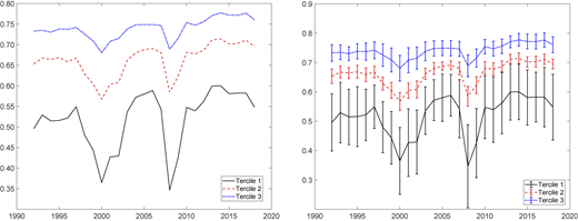
Beyond the statement of Hypothesis 2, expression (2) provides a separate prediction. When we observe a large variation in family firms' efficiency at certain periods (see Figure 4) the reason is that during those periods there is greater variation in family involvement or compensation. This is an interesting implication of our theory: it explains the “Why” of heterogeneity being at times higher and at other times lower. The causal logic is that after efficiency varies due to changes in family, company, and governance characteristics, the family firm responds with two mechanisms – family involvement and compensation. For a given firm, the greater the family involvement, the larger the negative impact on efficiency (Anderson and Reeb, 2004; Villalonga and Amit, 2006; Miller et al., 2007). And the greater the compensation, the larger the positive impact on efficiency (Gabaix and Landier, 2008).

A key component of our approach is efficiency. Intuitively, efficient firms maximize performance in some way, which varies depending on the type and objective of the firms. Following Kumbhakar and Lovell (2000), we measure family firm efficiency using stochastic frontiers. The methodology is an extension of regression that measures family firm efficiency and permits multidimensional components. It allows for varying degrees of success in pursuit of company objectives. To this end, stochastic frontiers measure the distance of each firm's performance from a hypothetical efficient level ^[2]. This method is attractive because it compares each family firm only to its best possible outcome. Moreover, it can incorporate multidimensional performance measures and is readily computed for longitudinal data.

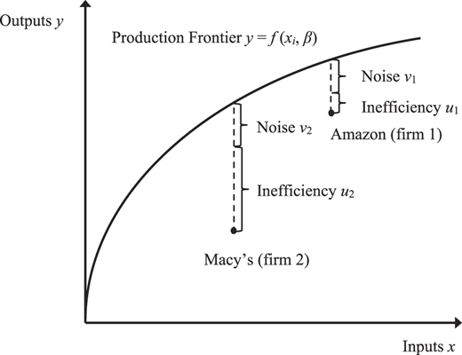
Graphical Intuition for our Approach to Firm Efficiency. Consider an hypothetical graph of Macy's and Amazon, in Figure 3. For given inputs x, the firms will produce some output y. However, the firms have different productive potentials, so it is important to compare them to their “best selves”. For example, if Amazon's maximal output is double that of Macy's, a raw comparison of the companies' output will not convey how successful they are at reaching their potential. The efficiency approach compares each company to the best output it could achieve, via the size of their efficiency terms u₁ and u₂.

Overview of Empirical Method. Our method of measuring efficiency is based on production functions. Suppose we have a sample of I firms and their inputs x_i, for i = 1, .., I. Then we can write their production function as y_i = f(x_i; β). PE_i, where y_i is the output of firm i, f(x_i; β) is the production frontier of all firms, and β is a vector of technology parameters. PE_i is the technical efficiency of family firm i. Rewriting the above equation, we express firm efficiency as

Thus, efficiency is the ratio of observed output to maximum feasible output. A condition for y_i to achieve its maximum f(x_i; β) is PE_i = 1. Otherwise PE_i < 1 measures the shortfall of observed production from the frontier.

In order to incorporate firm-specific random shocks, we specify a stochastic production frontier. This extends the above expression to include two firm-specific parts exp{v_i} and exp{u_i}, which capture randomness. The terms capture two types of firm randomness: the first term reflects luck, the second reflects firm inefficiency. Consequently, the expression for efficiency now becomes $PEi=yif(xi;β)⋅exp{vi}⋅exp{ui}$⁠. This latter definition of efficiency is the ratio of observed output to maximum feasible output, in a stochastic environment characterized by exp{v_i} and exp{u_i}. Intuitively, the setup allows firms to be inefficient at times, due to either bad luck (random shocks) v_i, or due to firm-specific inefficiency u_i. The key quantity that we estimate in the following analysis is PE_i. Additional details are available in an online Appendix.

Our data comprise variables related to company performance, which are available from the Compustat and Center for Research in Security Prices (CRSP) databases. The Compustat data are downloaded from the annual database while the CRSP data are downloaded from the daily database. In addition to these data, we hand collect information on the firms that are run by lone founders, in order to remove them from our sample. We thereby focus on firms that are run by several family members and face dynamic succession and kinship issues (Miller et al., 2007). We searched company websites, 10-K statements, and the internet for information on each of the potential family firms, in order to distinguish those firms that are run by lone founders. Using the same approach, we hand collected information on each firms' top management team, to assess family member involvement. We thereby build on recent research on family member involvement (De Massis et al., 2014). In particular, we first obtain the annual list of top management team members from Compustat's Execucomp database. We then research the profiles of team members in 10-K statements, company websites, and the internet, in order to determine who in the team are family members. This yields the FMT variable (FMT).

Data Sample. From Compustat, we extract and compute the following variables: ADV (expenses on advertising, divided by total sales); CAPEX (the ratio of capital expenditures to total sales); DEBT (the ratio of long-term debt to total assets); EBITDAAT (earnings before interest, taxes, depreciation, and amortization (EBITDA) divided by total assets); LNBE (the log of book value of shareholder's equity); LNME (the log of market value of shareholder's equity); MEBE (year end market-to-book ratio); PPEN (the ratio of property, plant and equipment to total assets); RND (expenses on research and development, divided by total sales); return on assets; and TNVR (the average monthly turnover of stocks during the fiscal year, where turnover is measured as trading volume divided by shares outstanding). In order to track firms and years, we extract the identifiers fyear (fiscal year) and gvkey (firm identifier).

From CRSP we extract the following variables: RET (average daily firm returns); SPRD (bid-ask spread); VOL (trading volume); and idiosyncratic volatility, denoted ivol. ivol is assessed by the Fama-French three-factor model, evaluated using daily returns over the fiscal year. The CRSP data identifier for each firm is its cusip, which is matched to the gvkey from Compustat, in order to combine information from the two databases. We extract the above data because they represent important variables from previous studies (Aggarwal and Samwick, 1999; Habib and Ljungqvist, 2005; Gabaix and Landier, 2008; Nguyen and Swanson, 2009). The sample spans fiscal years 1992–2018.

Data Filtering. The sample comprises firms listed on the New York Stock Exchange, American Stock Exchange or National Association of Securities Dealers Automated Quotations exchanges. For our methodology to be effective, we desire firms that are free to pursue efficiency objectives. Thus, financial and utility firms are excluded because they are highly regulated, and their estimated efficiency scores would not reflect optimizing behavior. We define family firms as those with at least five years classified as a family firm in the combined datasets of Anderson and Reeb (2003), and Anderson et al. (2012) ^[3]. Nonfamily firms are those with less than five years of this classification. As discussed above, we remove firms that are run by lone founders. While our focus is on family firms, we present information about family and nonfamily firms in the first two tables in order to place the research in context. Table 1 summarizes our data. The variables tend to have standard deviations of comparable magnitude to the means, and show a relatively wide range between minima and maxima. Therefore, the data possess substantial diversity, and are amenable to empirical analysis.

Benchmark Model. In a long panel inefficiency may vary over time and be confounded with firm effects. It is important to account separately for firm-specific effects, persistent inefficiency, and time-varying inefficiency. For example, if a panel model only includes firm-specific effects, this can confound inefficiency with firm characteristics that have no bearing on inefficiency. Alternatively, if a panel model completely separates firm effects from inefficiency, it may neglect persistent inefficiency that is specific to a family firm. In order to account for such issues, we follow Kumbhakar et al. (2014), estimating the frontier as

where lnme is the log of market value of shareholder equity. Based on Nguyen and Swanson (2009), our X variables reflect important economic considerations that impinge on corporation efficiency. As in Collins et al. (1997), we use LNBE (the log of book value of shareholder's equity) as a key accounting control variable that is relevant for market value of equity. We use DEBT (the ratio of long-term debt to total assets) to capture leverage considerations (Hanousek et al., 2015). We include CAPEX (the ratio of capital expenditures to total sales) to measure investment in tangible assets. PPEN (the ratio of property, plant and equipment to total assets) is utilized since a higher level of this variable can distinguish a traditional manufacturing firm from other firms that are close to the technology frontier. We include EBITDAAT (EBITDA divided by total assets) to measure operating profitability that is not affected by financing decisions.

Our key controls for investment in intangible assets comprise RND (expenses on research and development, divided by total sales) and ADV (expenses on advertising, divided by total sales). We include dummy variables XRD_D and XAD_D to represent missing observations on RND and ADV. When a particular observation is missing, the corresponding dummy variable is set to 0, otherwise it is set to 1. We also include dummies for the 48 Fama-French industries. Finally, the efficiency and family firm parameters are the following. θ_i, v_i, η_i and u_i are error terms representing firm effects, estimation error, persistent inefficiency, and transitory inefficiency, respectively ^[4]. As in Kumbhakar et al. (2014) we let β = [β₀, β_i], and then express the frontier as $lnmei,t=α0*+f(Xi;βi)+αi+εi,t$⁠, where $α0*=α0−E(ηi)−E(ui,t)$⁠; α_i = θ_i − η_i + E(η_i); and ɛ_i,t = v_i,t − u_i,t + E(u_i,t). Then the model is estimated in three Steps. First, a standard fixed effects model is used to estimate $βˆ$ and a residual $εˆ$⁠. Second, $εˆ$ is used to estimate time-varying inefficiency u_i,t from the relation ɛ_i,t = v_i,t − u_i,t + E(u_i,t). Third, similar to Step 2, we estimate persistent inefficiency η_i from the relation α_i = θ_i − η_i + E(η_i). After estimating the above terms, we construct overall family firm efficiency as the product of its time-varying and persistent efficiencies exp(−u_i,t|ɛ_i,t) and exp(−η_i). Further details are in Kumbhakar et al. (2014).

In stochastic frontier analysis, it is standard to impose functional form restrictions on the one-sided error term (Chapter 2, Kumbhakar and Lovell, 2000). We utilize a truncated normal model, similar to Battese and Coelli (1988). Estimation is performed by maximum likelihood. In order to allow for heterogeneity, we permit the standard deviation σ_u of the truncated normal distribution to depend on idiosyncratic volatility of firm returns, denoted ivol. Volatility has been argued to be a determinant of pay-performance efficiency (Aggarwal and Samwick (1999)), and Habib and Ljungqvist (2005) have used ivol in a similar manner for stochastic frontier estimation. We permit the standard deviation of the distribution to evolve according to σ_ui,t = δ₀ + δ₁ivol_i,t−1. ivol is computed as the standard deviation of excess returns from the Fama and French (1993) three-factor model, evaluated using daily returns over the fiscal year ^[5].

Table 2 presents estimates of the frontier model in (3), with separate models for family and nonfamily firms. The estimated coefficients accord with our intuition and are similar to previous results in efficiency research (Nguyen and Swanson, 2009). For the family firms all variables are strongly significant except RND. The coefficient on ivol is strongly significant. Hence, volatility-induced variation in efficiency is important. The Wald test indicates that the variables are jointly important for determining the frontier.

In Figure 4 we present graphs of average annual efficiency across family firms ^[6]. Each year we sort firms into three groups from lowest (Tercile 1) to highest efficiency (Tercile 3). The upper panel shows average efficiency in each tercile. The three terciles comove, all exhibiting substantial shortfalls around the recessionary periods of 2001 and 2008–2009. The lower panel shows one standard deviation bands around the tercile means. We observe ample heterogeneity, since the standard deviation bands for Tercile 1 and 3 look different. It is instructive to consider our results in monetary terms. The family firms' mean efficiency is 0.65, and average market capitalization is approximately $4.3 billion. Thus, if the average family firm improved efficiency to the maximum, it would enhance its market value by around $2.3 billion ^[7].

Testing Our Hypotheses. Recall our Hypotheses from Section 2. Hypothesis 1 says The Distributions of Family firm Efficiencies are Heterogeneous over time; Hypothesis 2 says Family Presence in the Management Team is Negatively related to Dynamic Family Firm Efficiency; Executive Compensation is Positively related to Dynamic Family Firm Efficiency.

Hypothesis 1: Tests of Heterogeneity. A standard way to assess heterogeneity is to test equality of means and variances. Table 3 presents our results. Panel A shows summary statistics on the efficiency terciles. There is a big jump in means from 0.5141 to 0.7375, when we move from the least to the most efficient family firms. Panel B tests for differences in means. The minute p-values indicate strong evidence against the null of equal means. In Panel C, the variance of each family firm tercile is statistically different from that of other terciles. Hence, we have strong evidence for Hypothesis 1: family firms exhibit dynamically heterogeneous efficiency.

Hypothesis 2: Tests of Dynamic Family Team and Compensation Effects. The DFM theory indicates that efficiency will vary over time differently for different family firms, because of time-induced changes in family factors, stewardship-agency, governance, and so forth. The central insight is that efficiency is negatively related to family presence in management, and positively related to CEO compensation. Besides compensation, we control for other CEO factors that affect efficiency: size of executive's ownership stake (shares in the company), life experience (age), and company experience (time working at the company). While there are other relevant aspects of family involvement and executive motivation, we focus on these four because they exhibit variation over time, and we can obtain measurements for them. The first two (compensation and ownership) are incentive based and free to vary with time. The latter two increase linearly with calendar time. Importantly, these variables are nonbinary; they are multi-valued and recorded at annual or higher frequency. Therefore, the data are appropriate for testing our theory. We also include binary controls for gender, whether the CEO sits on the board, whether the CEO was hired from outside the company, and the governance index of Bebchuk et al. (2009). In our tests, we impose a hurdle for CEO qualities to matter, by including time effects and family firm-specific effects – unobserved family firm attributes which may influence firm performance. If we find that executive variables and family involvement are significant it means that they matter for efficiency, over and above the influence of time and other family firm attributes.

Table 4 presents the results of 12 different empirical models, where family firm efficiency is regressed on family management involvement (FMT_D), executive compensation (LNCOMP), various CEO characteristics, and different combinations of time effects and fixed family firm effects. We discuss significance at the 95% level unless otherwise indicated. We do not include leverage, since that is already incorporated in the estimation of efficiency from Table 2. Consider model 1 (column 2), which comprises the smallest benchmark model with FMT_D and LNCOMP, four CEO characteristics, and time and firm fixed effects set to zero. In this case all of the CEO variables except shareholdings and gender are highly significant. Now consider model (4), where in addition to the CEO variables there are both time and firm effects. In this model compensation and several other CEO-related variables remain significant, while family management involvement and CEO involvement in the board of director become insignificant. This finding may be due to a situation where the latter two variables tend to be somewhat persistent, and are therefore already captured by fixed effects. Moving on to the other ten models, we observe that CEO's compensation is significant at the 99% level in all 12 specifications. And in nine of the models family involvement is significant. Interestingly, other CEO variables also matter in quite a few specifications, and although gender does not matter in the baseline model, once we control for fixed effects gender becomes significant. The F-tests are significant at the 99% level in all 12 models. Therefore we can confidently reject the null hypotheses that all parameters are zero. In sum, dynamic CEO compensation and family involvement in the management team are significantly related to dynamic family firm efficiency. This finding supports our Hypothesis 2.

A natural question concerns whether CEO qualities proxy for something else, such as firm size. We therefore redo the estimation from Table 4 with 12 additional models. The models are the same as before, except they include firm size. The results are in Table 5. In all except one model CEO compensation continues to be a significant determinant of efficiency. As before, family involvement in management remains significant in nine models. Thus we have strong evidence for Hypothesis 2: dynamic compensation and family involvement in management are strongly (and oppositely) related to dynamic efficiency. In an online Appendix we conduct a robustness study with propensity score matching to select similar family and non-family firms. Our previous results remain significant.

We provide a theoretical construct of dynamic family firm performance, the DFM theory. We use the theory to characterize dynamic heterogeneity in family firm efficiency, and offer a Family Involvement-CEO efficiency link. While family involvement and CEO compensation are used in static settings, it is novel to combine the two factors in a temporal model. We utilize a microfounded performance approach to construct efficiency for a longitudinal sample of multi-industry family firms ^[8], in order to address the question that guides our study: Do family involvement and executive compensation help to explain heterogeneity in family firm efficiency over time, and in opposite directions? When we test our model we find overwhelming evidence that changes in family firm efficiency are heterogeneous, and that family involvement and executive compensation are strongly (and oppositely) linked to efficiency, in support of our theory. Our theory also explains the “Why” behind heterogeneity being at times higher and at other times lower. When we observe large variation in family firms' efficiency at certain periods (see Figure 4), the reason is that during those periods there is greater variation in family involvement and compensation. Our model builds on previous research that highlights a positive relationship between CEO compensation and efficiency (Gabaix and Landier, 2008). Such research does not ascribe causation: the relation could arise because highly paid CEOs raise efficiency, or because firms that are more efficient can afford high compensation.

Theoretical and Empirical Contributions. We contribute to existing knowledge by opening up discussion on heterogeneity in the evolution of family firm efficiency, by offering a theoretical construct, and by presenting provocative evidence on the dynamics of efficiency. A novel theoretical insight is the countervailing link between efficiency and family involvement on the one hand, and efficiency and compensation on the other hand. These insights help to advance family business research and theorizing because our new reasoning and evidence raise questions that require extending existing frameworks. Previous research on family firm performance has tended to focus on specific industries or sample periods. There is a clear need for research that studies multiple industries, tests hypotheses in longitudinal data, and studies family firms and time. We make progress in these areas, and develop a dynamic theory of family firm performance. We test our theory on 25 years of longitudinal data that we construct, using a microfounded measure of family firm performance.

We also provide a benchmark for what to expect for family firm efficiency over time. The DFM model suggests that we can make successful inroads by focusing on three qualities: an initial Time Effect and mediating Family Team and Compensation Effects. The time effect leads to heterogeneity in efficiency over time, since both the family and firm evolve. The Family Team effect says that family involvement in management tends to worsen family firm efficiency. The Compensation effect says that large monetary incentives help the CEO improve efficiency dynamics. To the extent that CEO compensation and family involvement differ, we expect heterogeneous evolution in family firm efficiency over multiple periods. In particular, we should expect significant “gaps” between the most and least efficient family firms, both in means and variances. This is not obvious: one could plausibly argue that over time family firm efficiencies converge, since in an information economy effective management practices diffuse rapidly, and eventually more and more families settle on the best approach to handling their firms.

Moreover, our framework indicates that differences in the evolution of family firm efficiency are explainable to a large extent by three factors: time, which changes family relations and governance (e.g. succession, birth of children and death of founders, family conflicts, relation dynamics); CEO compensation; and family involvement in the management team. Two practical implications for family firms are that CEO compensation is valuable for efficiency management, since it matters in almost all empirical specifications; and management teams with mainly nonfamily members are often more effective at raising efficiency. These implications are detectable, despite the two effects operating simultaneously and in opposite directions. In sum, our approach provides a benchmark about what to expect in the evolution of family firm efficiency (large gaps in performance sustained over time); and suggests what can be done (incentivize CEOs with large compensation, and employ some nonfamily members in top management). As with most theoretical constructs, our model oversimplifies the complex family firm landscape. In reality, family firms must respect monetary and family barriers that restrict compensation and ability to hire outside CEOs. Family firms must also nourish non-financial aspirations such as family legacy. Moreover, other factors will determine family firm goals, such as firm size, geographical location, and the family's generational issues. Thus, the implications that we offer should be interpreted appropriately for the relevant context.

As mentioned in the Introduction, a body of important work touches on our research question, and may find our results useful. This work focuses on predictors of family firm performance, underscoring the roles of founders, number of employees and management style, and collective entrepreneurship. Founders strongly affect family firm performance, both financially and more broadly. Family firms perform better at founding, especially with independent directors (Anderson and Reeb, 2004). Survey evidence on small- and middle-sized enterprises founders shows that family involvement in the founder's firm affects outcomes including business performance, strategic planning, and satisfaction with business success (Powell and Eddleston, 2017). Another area concerns the relationship of employee numbers (“size”) to management styles. Empirical research documents that size explains important activity such as nonfamily members in management and family member conflicts (Sonfield and Lussier, 2008). The last area concerns collective entrepreneurship: synergistic activity from the family team, which searches for activities to deliver entrepreneurial progress. Yan and Sorenson (2003) posit that two factors influence collective entrepreneurship – family members' commitment to the firm; and collaboration among family members. The authors indicate a need for micro level studies and longitudinal analysis, which we provide. While influential, the foregoing work had gaps which we endeavor to fill. The above work could gain from our results, since we examine family firm performance in a micro-founded manner, and model and test the importance of dynamic family involvement in management. Moreover, we integrate previous work's insights in our dynamic model, which we validate using hand-collected data.

Limitations and Future Research. Despite our contributions, our paper has limitations. First, the theory could be enhanced by going into details of the family, including succession, and gleaning a deeper understanding of family characteristics that affect performance. Second, while our efficiency measure is multivariate, our main components reflect financial stakeholders (equity, debt) and consumer stakeholders (advertizing, R&D). We limited our measure to these categories in the interest of parsimony. It would be beneficial if other family firm performance measures were available. Third, while our sample is large and covers multiple industries, we consider only publicly traded US firms. Fourth, a natural question is whether our model reflects deeper endogeneity. Our focus was to build a workable model relating efficiency to compensation and family involvement, but it is worthwhile to consider an underlying dynamic factor that endogenously determines the variables. Fifth, we focus on disadvantages of family involvement for efficiency, while future research should highlight advantages of family involvement. Lastly, our theory and empirics show that dynamic CEO compensation and family involvement in the management team help to explain differences in family firm efficiency. Nevertheless, it is important to encompass other considerations such as power dispersion among family members.

We envision several growth areas for research. First, it is important to assess how family relations, firm characteristics, and stewardship-agency balance change over time. Second, efficiency can accommodate nonfinancial performance. Third, it would be useful to extend the study to private firms and data from other countries. Lastly, an intriguing possibility is to explore how other important dynamic family firm quantities – management styles, personalities, and family structure – affect temporal heterogeneity in performance.

Why are some family firms persistently more efficient than others? Family firm research has made great strides in understanding heterogeneity in a static setting; much remains to learn about dynamics. We develop a theory which posits that heterogeneity in efficiency arises due to time itself, which changes efficiency sources. Furthermore, changes in efficiency will be differentially managed depending on executive compensation and family involvement. Efficiency dynamics therefore depend on compensation and presence of family members in management. A counterintuitive aspect is that the two factors operate simultaneously, in opposite directions, and are still discernible.

It is not inevitable that substantial heterogeneity exist over time. Family firms experience forces that limit heterogeneity – bankruptcy to remove inefficient firms and regulation to reduce efficiency among the best firms. Our theory says, nevertheless, that dynamic variation in efficiency is significant, due to family firms' unique tools for managing inefficiency: compensation and family involvement in management. We evaluate our theory on longitudinal data of our own construction, comprising microfounded measures of family firm efficiency, and hand collected information on family involvement in management. We document substantial heterogeneity in efficiency over time. Dynamic efficiency is typically negatively related to family involvement and positively related to compensation, in support of our DFM theory. Future work may extend our research, deepening our understanding of family firm heterogeneity in dynamic settings.

The supplementary material for this article can be found online.