Implementation of a physics-informed neural network to predict relative densities for copper LPBF with a green laser system

In recent years, there has been an increase in research regarding the use of copper within the laser powder bed fusion (LPBF) process. While many addressed copper alloys, pure copper has also sparked high interest because of its excellent thermal and electrical properties for industrial use. Because of the geometric flexibility through the LPBF process, there are many more possibilities to effectively use these properties, especially in demanding fields such as aerospace and aviation. However, these studies have almost exclusively focused on the optimization of the relative density of copper by changing printing parameters through an excessive number of experiments. Some studies have also measured mechanical and electrical properties of the printed copper samples; few to none have examined the effect of heat treatment or other post processes on these properties. This study aims to present and analyze a method which poses the opportunity to reduce the experimental effort during the determination of feasible process parameters for challenging materials. The primary goal is to modify and use physics-informed neural networks (PINN) to predict the relative densities of copper samples given specific parameters.

This study will serve as an initial step toward the ability to adapt the LPBF more commonly, as it becomes easier to process different materials and parts. Through the ability to predict relative densities, future achievements may involve the targeted influence of the microstructure, such as grain sizes, shapes and direction and, thus, the functional and mechanical properties, while maintaining high density. Providing parameters in a fast way to allow the in-situ tailoring during the process could additionally lead to the opportunity to produce parts that possess different functional properties in different areas, optimizing the usability and efficiency of these parts. This enables the production of parts with combinations of different properties using pure copper. Post-processing could be reduced or omitted. Therefore, the application of the PINN method in this context has huge implications on sustainable lean process development, as it allows a substantial reduction in the number of experiments necessary to achieve the desired results. Fewer experiments lead to less material usage and waste regarding powder material, less production time necessary on costly LPBF systems and less time spend by a highly qualified and, therefore, costly workforce. The usage of consumables and supplies like personal protective equipment and inert gas is also reduced. A lean process development additionally saves time in the product development process, if PINN are used to enable the manufacturing of challenging parts.

Pure copper is a functional material that is often used because of its high thermal and electrical conductivity, making excellent heat exchangers and electrical devices (Ikeshoji et al., 2018). As the manufacturing industry is rapidly evolving, higher requirements are set. Combined with complex geometries through LPBF, the potential for copper parts which combine the functional properties of copper with the advantages posed by LPBF is very high (Jadhav et al., 2019). This becomes evident by the high number of applications realized through LPBF of copper, which include heat exchangers using lattice structures, electrical machines, electrical coils or heat sinks. One of the most important applications for pure copper is heat exchangers, which are both needed in automotive and aerospace manufacturing, among many other fields. Because of the flexibility regarding complex geometries, the individual specific requirements can be met while using the minimal amount of material, making copper parts especially useful for aerospace engineering, where lightweight components are essential. Another application is copper coils used in electrical motors, which can be customized to achieve the optimum use of space, therefore reducing the size and weight of those and possibly increasing the power (El-Wardany et al., 2018; Silbernagel et al., 2019; Constantin et al., 2020; Ho et al., 2020). Besides geometrical advantages, the high material efficiency, production on demand and the possibility to manufacture without tools add to possible improvements with AM processes. The customization of products without resulting in high costs is an additional benefit of AM.

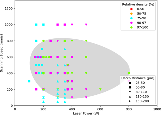
However, regarding conventional LPBF, this process is primarily suited for materials that have low reflectivity and low thermal conductivity. This means that pure copper is not an optimal material because of its contrary properties. Copper has an extremely low laser absorption rate near the infrared wavelength $λ$ of approximately $1060…1080 nm$⁠, which is commonly used by many LPBF systems (Hummel et al., 2021). Copper’s high reflectivity and high thermal conductivity reduce the energy that is available for the melting of the copper powder, limiting the maximum local temperature. This results in defects in the finished product, with porous parts lowering the relative density. Poor mechanical and electrical properties of additively manufactured copper parts are detrimental to the wider usage in the industry. Because of this, many studies in the past have examined LPBF with mixed copper powders, as these alloys allow for better laser absorption and thus higher densities. Copper alloys are also associated with higher mechanical properties but perform lower regarding functional properties like thermal and electrical conductivity. Therefore, especially in electrical engineering, where the electrical and thermal conductivity of copper is essential, the use of pure copper is indispensable. The usage of high-powered laser systems or systems with a laser wavelength $λ$ in the green light spectrum around $532 nm$ are two applied possibilities to manufacture pure copper via LPBF. The various strategies to achieve high-quality parts applied to a variety of copper alloys and with different LPBF systems result in a diverse range of used parameters and process performance presented in the literature. Figure 1 emphasizes this fact by showing the various process parameters used by different working groups to additively manufacture pure copper and copper alloys like CuCrZr, Cu10Sn, CuCr, CuCr30, CuGr and CuSn. The combined data of process parameters and resulting relative density is extracted from available research articles. It is clear that different parameter combinations are effective. However, influences such as the scanning strategy are not considered despite the consideration of key process variables and have an influence on the energy input in relation to time. The large variance in the process results also shows that the repeatable and transferable achievement of dense components is a current challenge. The general trend in Figure 1 shows that higher relative densities are possible through process parameters that generate a higher energy density. If manufactured with a low number of defects, then the high geometric flexibility of LPBF can increase the electrical and thermal performance of copper components, as that is not only determined by material properties such as electrical and thermal conductivity but also by the geometric design. LPBF, therefore, shows great potential to not only increase the electrical and thermal performance from a microstructural way but also from the geometry perspective – with more design opportunities in AM. The research analyzed to create Figure 1 is listed in Table 10 in the supplementary material to this article.

Although LPBF has reached a high state of technology maturity, several challenges regarding the productivity but especially the repeatability of processes remain. Implementing stable processes initially is difficult without a high number of tests and analysis of the process results. The large number of standards in the field of AM recently published underline the need for standardization and stable processes (Riccio, 2021). The efforts of testing and analysis necessary to produce parts and specimens with a high quality from challenging materials show the need for research to optimize this process (Safaei et al., 2021). Additionally, the known relationships between process parameters are not reliably part of process studies and are, therefore, not considered. To establish quality assurance processes that consider a sufficient number of parameters, machine learning (ML) can pose an opportunity (Taherkhani et al., 2023). After process parameters are found that lead to an acceptable quality, the reliable achievement of this quality is not ensured, as machine and process conditions are subject to changes. Even if a process runs reliably, the transfer between systems, machines and production facilities relates to an effort to ensure that the process meets the required demands. Identical parameters lead to different results. Drifts in subsystems of a LPBF machine, for example, the laser, lead to a changing behavior over time (Narasimharaju et al., 2022).

PINNs are a method of ML that differs from conventional methods by considering physical laws besides pure or simple data sets (Raissi et al., 2019). It does not derive the solution purely based on data, making it more robust, especially in the engineering context. In the conventional method of ML, extremely large amounts of training data are used for the neural network (NN). A common issue in the research of NN is the lack of generalization, making it difficult to simulate more complex models (Moseley et al., 2020). For any inputs outside of the training distribution, the results will be unreliable. The approach of further increasing the training data is not feasible, as it is costly and time consuming. In many practical settings, either only limited data is available or the experiment observations are noisy. Instead, PINNs use the already existing physical knowledge, which provides further constraints that the PINNs must satisfy (Raissi et al., 2019). This provides a more scientific approach, eliminating results that are physically impossible, thus reducing the possible solutions to reasonable amount. These laws and principles of physics are used through mathematical models, more precisely partial differential equations (PDEs) (Cuomo et al., 2022). This reduces the data sets needed to train the NN immensely, as it also increases the informational value of the available data (Raissi et al., 2019). The more physical knowledge is included, the less data are needed, which is costly to obtain.

PINN can be seen as an extension of NN. Cuomo et al. describe PINN in three sections: a NN, a physics-informed network (PIN) and a feedback mechanism (Cuomo et al., 2022). Artificial NNs (ANNs) are ML techniques that simulate biological organisms through neurons. These neurons can receive inputs and send out outputs. Multiple neurons make up a layer. The basic structure of an ANN consists of an input layer, at least one hidden layer, and an output layer as seen in Figure 8 in the supplementary material to this article. In general, ANN can be differentiated between shallow ANN and deep NN. One difference is that while shallow ANNs only have one hidden layer, deep NNs have multiple, allowing them to model more complicated relationships (Aggarwal, 2018).

Each input for a neuron is multiplied with a weight. The weighted sum of all inputs for a specific neuron goes through an activation function. The output then serves as an input for the next neuron. The choice of activation functions is an important factor in the design of the ANN. Depending on the purpose, different activation functions can be applied, such as the tanh or sigmoid function (Aggarwal, 2018). Sharma et al. present an overview of activation functions, which are important as they can present non-linearity to the ANN, enabling it to take on complex, non-linear relationships (Sharma et al., 2020). The input weights are modified based on how well the prediction matches the training data. That is done through a loss function and can be described as the feedback mechanism (Cuomo et al., 2022). The loss function evaluates the accuracy of the ANN based on the training data. It compares the predicted value with the actual value. While there are different possibilities to model a loss function, the most common choice across different fields is through a mean square error (MSE) (Zhao et al., 2015). The goal of the training is to minimize the loss function, consequently minimizing the error. That can be done by backpropagation, which is the process of adjusting the weights based on their influence on the overall loss. This learning algorithm of the ANN is basically a gradient descent optimization algorithm, which is constantly repeated to find the optimal weights to receive accurate predictions.

Using the designations proposed by Cuomo et al., the PIN represents the functional component of the PINN and overlaps with the NN (Cuomo et al., 2022). It contains the information regarding physical knowledge in the form of PDE. PDE depict the non-linear relationship between a variable, such as a parameter, and its partial derivatives to time and space. In the context of PINN, PDEs describe the physical knowledge in form of mathematical models. It is important to keep in mind that these mathematical models are only approximations, meaning that PDEs are only an incomplete representation of the real complex physical process. Because ANN can derive real relationships from the data sets, the interplay between ANN and PDE can form a more reliable model (Kapusuzoglu and Mahadevan, 2020).

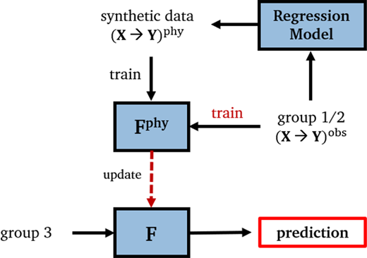
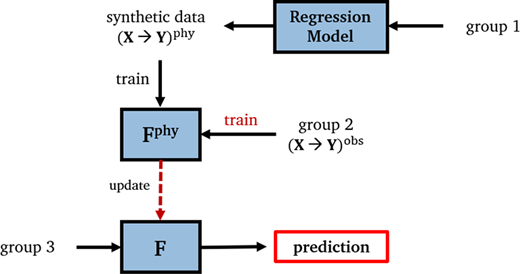
Kapusuzoglu and Mahadevan (2020) proposed different approaches to consider PDE in PINN in the context of AM. In one technique, the physical knowledge is used for the pretraining of the ANN. This means synthetic data $Xphy$ is generated, using the physics models. $Xphy$ is used to pretrain the ANN$Fphy$⁠, and afterwards, $Fphy$ is trained with the experimental data sets $X$⁠, updating the ANN to $F$⁠. The initial weights chosen are already considerably fitted based on the pretraining, so the experimental data merely upgrades and fine-tunes the weights, reducing the amount of data needed. Here, the PDEs are only used for this initialization and play no further role in the training process. It has been shown that even faulty physics models can reduce the amount of experimental data needed (Jia et al., 2021). Another advantage is that the synthetic data from PDE covers a wide array of data, which is not possible with expensive experiments. This allows the PINN to have a wider generalization, surpassing the range of experimental data (Kapusuzoglu and Mahadevan, 2020). This makes this method most suitable for this research concerning pure copper LPBF.

To summarize, the goal of the PINN is to predict a solution $Y^$⁠, using the weights $ω$⁠. These weights $ω$ must be chosen, so that $Y^$ is as close to the actual value $Y$ as possible, thus minimizing the error through the loss function $1n∑nY-Y^2$⁠.

ANN can be differentiated into two different types: feedforward NN and recurrent NN (RNN). The difference between them is that RNN have feedback loops, through which they consider the information from previous inputs. Instead of a one-directional information flow from input to output, a RNN uses the output from a previous call again as input for the same node in the NN through these recurrent feedback loops. With every additional input, the memory of the RNN is updated, which allows the network to consider the context and certain behaviors (Salehinejad et al., 2018). Thus, every past input is considered in the prediction of RNN.

Wenzel et al. (2022) have proposed a method that aims at optimizing the system reliability in AM using a PINN. The goal is to predict outcomes and suggest input variables for different requirements. This is applied to a fused filament fabrication process, to prevent manufacturing defects. When tested on several fused filament fabrication machines as a case study, they found that the pretrained PINN had a 50–100 times lower root mean square error (RMSE) when predicting unknown experiments with very few experimental data than the conventional statistical approach. However, while the statistical approach increased in reliability with an increase in experimental data, the PINN approach stopped being effective after a certain amount of training data. They observed that at around 1,000 measurements from experiments, the RMSE was the same for both approaches (Wenzel et al., 2022).

All specimens which are used for training and testing of the implemented PINN and are not taken from existing research are manufactured on a powder bed fusion system by Aconity3D GmbH, Germany. Specimens are manufactured on a stainless-steel substrate plate with a diameter of 170 mm. The laser system is manufactured by IPG Photonics, the USA. The laser operates with a wavelength of approximately 532 nm and a maximum output power of 193 W. For manufacturing of the specimens, a linear scanning strategy was applied, and the scan vectors were rotated for 67° after every layer. Further comprehensive information regarding the analysis of the specimens, type and appearance of defects and resulting properties of the specimens other than relative density are available in a supporting study (Schäfle et al., 2025).

In this study, a newly developed PINN approach is used to predict relative densities of pure copper specimens after manufacturing via LPBF. The predictions are made based on a specific set of process parameters, which are important for controlling the process outcome. The usage of PINN is intended to reduce the necessary number of experiments when implementing a new process with a material which is challenging to use without producing defects or with other disturbances. This could include setting up a LPBF system at a new location or after retrofitting to a high extend. From a LPBF system, 52 data sets with a 532 nm laser at the research facility of the Institute for Product Development and Machine Elements (PMD) at Technical University of Darmstadt are used for training and testing of the PINN. Additionally, 160 data sets from published research regarding the AM of copper are used for testing the approach and pretraining the PINN. The relative density of the specimens manufactured by PMD is determined by optical analysis. A picture of the metallographically prepared specimen is taken per microscope. The picture is converted into a grey value picture. The black appearing defect spots are separated from the white background, and their area is measured, which is compared to the whole cross-section area.

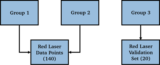
The predictions from the developed PINN are compared to other prediction methods commonly used in data science. A conventional ANN is constructed, which is trained with 140 data points from published research for red lasers. This data is also used for the training of the PINN. The ANN is tested with on the same 20 data points, which are also used as a validation set for the red laser PINN as referred to in Figure 2. This allows for a comparison of the performance regarding the quality of the estimations. The architecture as shown in Table 1 is implemented, with the only difference that the number of epochs is increased to 100, as 30 epochs do not provide sufficient training in this case because of the low amount of training data. As a second method for comparison, a linear regression (LR) is applied using the 140 data points from Groups 1 / 2 to predict the validation set (Figure 2). To ensure that the accuracy of the predictions does not purely rely on chance, the validation set is predicted five times for each method. The mean values of these predictions are then used for the following error measures.

To evaluate the predicted relative densities, the error measure of MSE in percentage points is used as calculated in equation (1):

For the first application of the PINN method on the LPBF process, literature data from previous studies with red lasers is used. That literature data is divided into three groups. One group is used as the domain knowledge to create a physical model that generates the data for the pretraining of the PINN. The second group is used for the PINN training. Here, data sets from published research are used, to investigate the feasibility of the developed approach for general usage, besides the application on a specific process. The third group will be used as a test set, to test if predictions from the trained PINN are accurate. The third group consists of literature data, which is consciously held back from the training process of the PINN. After training, the PINN is tested with parameters from the literature, and the results are compared to the findings in the corresponding studies.

There are six input parameters used in total: laser power, scanning speed, hatch distance, laser spot diameter, layer thickness and average powder size, which is taken from the powder size distribution. If the value is given in the respective research paper, then the $d50$ distribution of the PSD is taken. If not, then the mean value of that distribution is taken as an approximation. The goal value or output parameter aimed to be predicted is the relative density.

The behavioral vector is an informational variable, which retains the information about the behavior of the system. It needs to be defined, as it influences the number of neurons for the input layer of the PINN architecture (Wenzel et al., 2022). In this study, the value is set to 5.

A complete overview of the 160 used data sets from published research is provided in the supplementary material to this article. The literature data is split into the previously described three groups using random sampling. From the first group of data, a physical model for the pretraining of the PINN is created. A regression model is built using that group of data, so the data generated from this model follows the patterns of the domain knowledge. Apart from the direct effect of the individual input parameters on the relative density, the interaction effects between the input parameters have to be considered as well. The main effect and interaction effect together make up the total effect. The interaction effects are extremely important, as they explain the joint influence of multiple input parameters on the output (Wenzel et al., 2022).

The reliability of the regression model depends on the number of measurements used to create that model. The available data is extremely limited. In this special case, the data used to create the regression model can be reused for the training of the PINN, as the measurements themselves are not used for the pretraining. Only the data generated from the regression model is used there. In all, 140 measurements are used for both the regression model and the training of the PINN. The remaining 20 measurements will be used for the verification of the method, as illustrated in Figure 2.

Random forest regression is used as the regression model, and the applied parameters are stated in Table 4 (supplementary material), which is included in the supplementary material to this article. This model uses the average of the predictions of multiple decision trees that are generated based on random sampling of the data sets. This ensures that different data is used for every decision tree. These decision trees are independent from each other (Breiman, 2001). Because multiple predictions are used here and then averaged, the random forest regression produces highly accurate predictions. For the input parameters, random values are generated, which are restricted within a given range, depicted in Table 5 in the supplementary material.

For the regression model, two main parameters are of importance: the MSE and R-squared (R²), which is the coefficient of determination. The latter describes how much of the variance of the dependent variable (output: relative density) can be explained by the independent variables (input: laser power, scanning speed, hatch distance, laser spot diameter, layer thickness and powder size). The more data is used for the regression model, the better both parameters will be. To determine these parameters, the data is split into two sets: a training set and a testing set. The size of the test set is set to 20%, so 28 measurements are used for testing. The MSE and R² are determined using the generated outputs through the regression model and the test set. The parameters for this regression model are shown in Table 3, which serve as sufficient values for a reliable model.

The summary of the application of the method using the respective data sets is depicted in Figure 3.

For the pretraining of the PINNs, 10,000 data points are generated from the regression model and taken as input and output parameters, which must be normalized to values between $0$ and $1$⁠. A logarithmic normalization is chosen for the relative density. A linear normalization is impractical for the relative density, as relative densities of 70% or 75% are equally undesirable, but densities between 95% and 99% are considerably different. The percentages are taken as absolute values for the unnormalized data. In all, 70% relative density is chosen to be the minimum value, as there is no literature data showing densities lower than that. In all, 70% relative density serves as the lower bound and a 100% relative density as the upper bound. Because values closer to 100% should be spread more widely than values closer to 70%, an inversion of the values is carried out. This means initially, values closer to 0 are the higher relative densities and values closer to 1 are the lower relative densities. This is done through subtracting the density values and the upper and lower bound values from 101 within the logarithm function. This is explained by the fact that this results in the transformation of values between 0 and 1, as log(1) = 0. To reverse the induced inversion, all calculated values are ultimately subtracted from 1. Table 7 (supplementary material) contains examples of unnormalized and normalized data.

The normalized output data Y^phy is calculated as seen in equation 2. Table 7 in the supplementary material to this article shows the comparison between unnormalized and normalized data, depicting how relative densities closer to 100% are more widely spread through the normalization:

The input parameters are linearly normalized, each using the highest sensible value as the upper bound UB and the lowest sensible value as the lower bound LB as shown in equation 3 and summarized in Table 5 in the supplementary material. Of course, for different applications such as LPBF using a green laser or the LPBF fabrication of other metals, the upper and lower bounds must be adjusted accordingly. For the green laser, these bounds are summarized in Table 6 in the supplementary material:

This interpolated and normalized data is used as the physical training data $(X → Y)phy$ necessary for pretraining the PINN, which results in the PINN F^phy. The NN configurations for this step are identical to those used during the training of the PINN and will be described in detail in the corresponding following section. For the calibration of the PINN, the second set of literature experimental data is used, which in this case are the 140 measurements also used to build the regression model. After normalization, this is the observational data $(X→Y)obs$⁠.

In the same manner as for the pretraining, the input and output variables of the observational data are normalized to values between 0 and 1. This observational training data $(X→Y)obs$ is used to train the pretrained PINN F^phy, updating it to F.

To train the PINN, there are certain hyperparameters that can be adjusted, as well as the network architecture. The latter describes how the NN is structured: the number of layers, the number of neurons and the activation function in each respective layer. The adjustment of hyperparameters is important, as it influences both the time and performance of the training. They are set before the training. For this application, the architecture is set to five layers in total: There are three hidden layers and one input and output layer each. The reason for this is that the number of layers is dependent on the level of complexity necessary. Restricting the number of layers to a necessary level is important to prevent complications such as an excessive training time or overfitting. A possible approach is to start as simple as possible and gradually increase the number of layers until no further improvements are achieved or even degradation takes place. For all neurons of the hidden and output layer, the sigmoid function is used as the activation function, which is a function existing between 0 and 1 and is very commonly used in NN.

A summary of the PINN architecture can be found in Table 1, where the parameters of the architecture are summarized. The number of neurons is chosen randomly. The number of neurons in the input layer is determined as the number of features, which is defined as the number of input parameters added with the size of the compressed behavior vector (CVF). The output layer is defined to contain one neuron, because the developed PINN has one output.

Additional hyperparameters of the PINN are depicted in Table 2 and are optimized regarding training and validation loss.

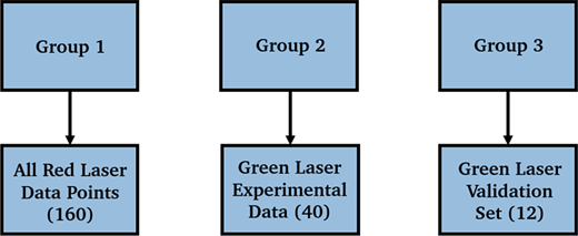
The transferability of the method to the LPBF process with green lasers is tested to determine if the physical knowledge about red laser LPBF processes can be used for pretraining the PINN for green lasers. All 160 data points for red lasers will make up Group 1, while the data points available for green lasers will be split into Groups 2 and 3, as shown in Figure 4.

The same regression model as before is used, this time using all 160 available data points from literature. This results in the regression parameters shown in Table 3. Figure 5 illustrates the functional principle of the PINN for predictions of green laser process outcomes, using the data groups in Figure 4.

The pretraining of the PINN is done as previously described, using the 10,000 generated and normalized synthetic physical data points $(X→Y)phy$ from the upgraded regression model.

For the training of the PINN, Group 2 is used which consists of 40 data points taken from an experimental study using a green laser. Because of significant differences in the parameters between studies with red lasers and studies with green lasers, these 40 data points are normalized using the upper and lower bounds shown in Table 5 (see supplementary material to this article). These observational data points $(X → Y)obs$ are then used as input to update F^phy to F. The PINN consists of the architecture described in Tables 1 and 2.

The trained PINNs are used to generate predictions for the relative densities of process parameter sets, retained from the training process. The results for these validation sets are compared to the known experimental results.

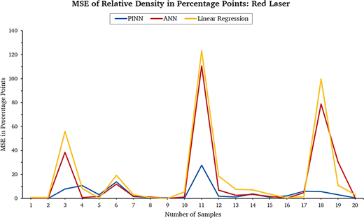
The red laser validation set of 20 data sets from Figure 2 is described in Table 13 (supplementary material), based on the data in Table 12 (supplementary material) which is taken from the literature listed in Table 11 (supplementary material). All these referenced tables can be found in the supplementary material to this article. The predictions for the relative density resulting from the process parameters are visualized for the applied PINN, the generic ANN and a LR in Figure 6 based on the MSE of the predictions versus the real result. The abscissa shows the number of the tested data set, which is derived from the numbering of the data sets in Table 12 (supplementary material), whereby the lowest number is assigned 1 and the highest 20. The ordinate shows the absolute deviation in percentage points between the prediction of the method used and the actual value for the relative density in percent. A deviation of approximately 30 percentage points as in sample 11 for the PINN, therefore, means that the amount of the difference between the predicted and actual relative density in percent is 30. All predictions made are summarized in Table 14 in the supplementary material.

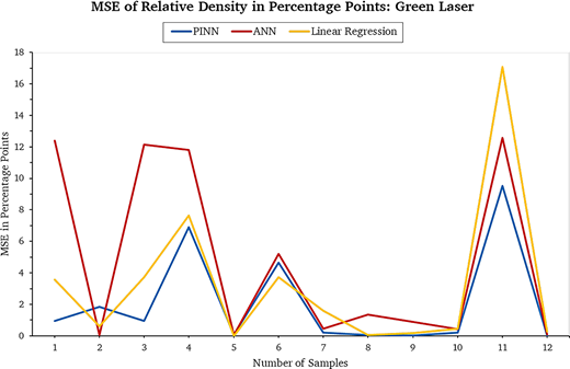
In the same way as described for the red laser, the PINN trained for application on green laser data is tested. In the supplementary material to this article, the relevant data is summarized: The 12 data sets shown in Table 16 (supplementary material) are picked from Table 15 (supplementary material) and are also referenced to in Figure 4. The predictions made are shown in Table 17 (supplementary material). Notably, the only difference between the red and green laser PINN is an increase in the number of epochs to 200, which is necessary to provide sufficient training, given that the amount of training data is reduced. As well as Figure 6, Figure 7 illustrates the relative differences between predictions and actual results based on the MSE. Similarly to Figure 6, PINN shows the smallest differences between predicted relative density values and experimental results.

The results of this study show clearly the overall capability of the application of a PINN on the prediction of process results for the LPBF process, demonstrated on the example of the processing of copper. But there are several factors influencing the results of this study, which need to be addressed to draw the correct conclusions and asses further applications of this method.

An important prerequisite for the functionality of the implemented PINN is that the process parameters used as input values are usable for the prediction of the relative density, resulting from a LPBF process. This necessary relationship for critical parameters like the laser power, the laser scanning speed, the hatch distance and laser spot diameter and the process result in the form of the relative density is well researched and established (Jiang et al., 2021; Shen et al., 2023; Srikanth et al., 2024; Chowdhury et al., 2022). Although other parameters could additionally be considered, the parameters used for this study are the ones most importantly and often considered during process development studies. Based on the results of this study, a sophisticated base for a process development can be determined, with the most critical parameters determined before starting initial experiments. This reduces the number of necessary experiments during process development significantly.

Another key aspect is the determination of the used parameters as well as the measurement of the process result in the form of the relative density. There are systematical deviations in the results of different relative density measurement techniques as well as additional varying measurement errors (Spierings et al., 2011). Data is extracted from different research publications from varying research environments and system set-ups. The used methodology for measurements differs between research groups. Considering the necessary high precision regarding the analysis of the relative density, the data from the literature cannot be fully relied upon. The performance of the PINN relies on the quality of the training data used; therefore, errors of the prediction can be partly attributed to a diminished quality of input data.

While the values of the process parameters can be adjusted precisely, there are deviations between the chosen machine settings and the real values. This is partly because of a limited capability of manufacturing systems regarding precision and repeatability and process irregularities (Dowling et al., 2020). Irregularities can include changes in the powder bed and the positioning of the parts on the build plate, influencing the laser interaction as well as drifts, for example in the laser characteristics (Yavari et al., 2021; Graybill, 2022).

It is apparent from the resulting prediction accuracy visualized in Figures 6 and 7 that the PINN stands out as the most precise method for predicting relative densities, outperforming the traditional methods ANN and LR. This is the case for predictions regarding red, as well as green laser systems. For data points that all three methods predict poorly, the PINN shows for the most part also smaller deviations than the other methods. The occurrence of peaks in the MSE is consistent between all methods. The PINN method does not exhibit peaks as pronounced as the other two methods. This suggests that the PINN method can handle complexity, as well as potential outliers, better. The reason for partly similar performances of the ANN and LR can be found in their respective functional principle and the data itself. It is highly likely that precise predictions from the ANN are made for datapoints that fit overall trends in the data well and stem from process regimes which are more densely backed up with data. Deviations for predictions of the ANN are likely to occur where known process knowledge is scarce or cannot be applied. The LR behaves in a similar fashion, as some data sets follow linear relationships based on the experiment design in which they were obtained. In addition, the stated reasons are highly likely explanations for the rare cases where the PINN is outperformed by the other methods.

Table 8 in the supplementary material to this article summarizes the determined performance indicators MSE and RMSE for all three methods for predictions of the red laser process. The values marked with an asterisk in Table 8 (supplementary material) demonstrate a case in which data point 11 was eliminated to show the difference one potential outlier or measurement error can make. This is done with the purpose of providing an understanding of these measurement uncertainties and to explore the possible thought that the predicted values could be closer to the truth than the literature data. The RMSE in Table 8 (supplementary material) can be interpreted as the average deviation, in terms of percentage points, between the estimated relative density and the real relative density of any previously unknown parameter set across the conditions of all ten research papers. Therefore, the PINN RMSE of 2.14 while including all validation data points represents an extremely good outcome given the challenges and complexity involved. Even better results are expected when using self-conducted data for training.

As Table 9 in the supplementary material shows, the difference in MSE among the three methods is less noticeable. A simple LR produces excellent predictions that are only slightly inferior compared to those of the PINN. The reason for this could lie in the lower complexity regarding the experimental data. The use data was taken from the process development for a green laser system. As the aim was not to provide a wide variety of data, rather than achieving a high relative density based on existing knowledge, the variation in the applied parameters is lower than what is provided by published research. Only three of the six input parameters for the green laser exhibit variations, while the other three are constant throughout all data points. This reduces the effective number of input parameters to three. Furthermore, unlike the previous scenario with red laser from literature, all data points in this case come from the same machine and are subject to the same environmental conditions as well as identical procedures for measurement. Overall, the experimental design of the process development on the green laser contributes to the fact that predictions can be made using LR because of the small variations in the input parameters. This is reflected in the overall lower error values, as evident when comparing the scaling of the ordinate between Figures 6 and 7 and the importance of consistent conditions and reliable measurements during data collection for PINN is underlined.

The PINN still yields slightly superior predictions with only a mean deviation of 1.46 percentage points, especially when directly compared to the ANN, as stated in Table 9 (supplementary material). This shows that the transfer of knowledge from literature data concerning red lasers proves effective in pretraining and ultimately positively influences the training process. This is reflected in not only the need for 170 additional epochs in the simple ANN but also the accuracy of the predictions.

The poor prediction for sample 11 in Figure 6 or deviations between the experiments and predictions in Figure 7 could be attributed to the absence of similar parameter sets in the training data. While the trend of the prediction is accurate, the model seems to overestimate the relative density, as it lacks information on even lower values. It is difficult to determine the exact reasons for the occurrence of strongly deviating PINN predictions. PINNs based on the integration of physical laws can create more transparency in the interpretation of results (Sharma et al., 2024). As the physical basis for predictions in the presented approach is given by real data, which is further enriched artificially, this possibility of differently structured PINN unfortunately does not exist here. Based on the principle of functionality of the applied PINN approach as presented in Figure 5, it is possible to reduce the negative effects of a small number of training samples in certain process regimes. The generation of artificial data cannot fully compensate for lacking data, especially if marginal areas of the process regime are affected, as non-linear effects occur which cannot be mapped by the LR model used for artificial data generation without experimental enrichment. The generalizability and numerical stability of PINN models are general issues necessary to address in the future to facilitate the broader use of PINN in AM and generally and to make use of their full potential (Farrag et al., 2025). However, the comparison between models shows that the PINN was able to deal with this information gap the best.

But even in light of possible influences on the predictions made by the implemented PINN, a significant potential of the presented approach on the process development of challenging additive manufacturing processes has to be acknowledged. Based on existing data from similar processes and a limited amount of experimental effort, high quality predictions are possible. This shows that the implemented PINN approach can be part of a future leaner process development. The presented results are in line with related research, which shows improvements in predictions of process results and process conditions with augmented neural networks. For the prediction of defect behavior under cyclic loading, the fatigue life of additively manufactured parts can be made significantly more accurate with the application of a PINN using physical constraints, as well as the prediction of thermal process conditions (Feng et al., 2025; Zhu et al., 2021). Studies with a focus on a broader review of the PINN technology in AM show that while challenges remain, the facilitation of process control and fast adjustments and a possible reduction in the reliance on extensive training data can be expected to improve manufacturing efficiency (Farrag et al., 2025).

The findings of this study establish the superiority of the PINN method over simpler models such as a basic ANN or LR in the predictive accuracy of relative densities when given the process parameters. The application of this method was conducted for the LPBF process of copper, using red laser data from literature and experimental green laser data.

The following conclusions can be drawn:

• The developed PINN approach for the prediction of process outcomes based on parameters of the LPBF process shows a high accuracy and is more accurate than a conventional ANN, as well as predictions based on a LR.

• In all scenarios tested, the PINN yields the most accurate predictions. It especially excels in handling data sets that possess high complexity or are very limited.

• The employment of red laser data for pretraining in scenarios involving green laser data demonstrates that the transfer of knowledge from experiments involving red lasers to experiments with green lasers is feasible.

The research presented offers several starting points for continuing the approach of using PINN in additive manufacturing. One possible approach is the expansion of the PINN predictions on more properties of finished parts and specimens after LPBF. With additional data, predictions like the presented ones for the relative density should be possible for mechanical and functional properties, or the resulting microstructure. Another possibility is the application of this PINN approach on the process development of other materials, by including information about the chemical composition and absorptivity together with process results. As shown, with a limited number of experiments, predictions about feasible process regimes should be possible.

The supplementary material for this article can be found online.