The potential of machine learning modeling to predict urban construction transport demand

The construction transport represents between 20–35% of urban freight traffic in European cities and a similar share of transported tonnages in a city (Brusselaers et al., 2020; Dablanc, 2008). One tends to treat construction projects as a time-limited disruption. However, as cities are constantly evolving and densifying, they continuously call for new construction, renovation, and demolition projects. A city therefore continuously attracts construction-related transport flows, with varying construction site locations and durations (Brusselaers et al., 2023a, b; Fredriksson et al., 2022). Given the changing sites’ locations, durations and characteristics, there is also a growing need to predict how much construction transport demand will be generated, to enhance a city’s traffic planning.

Traffic planners often deploy freight transport simulation models to analyze the impact on a city’s traffic network. Generating a demand for freight transport is the first part in creating a freight generation model. However, overall freight transport flow data is scarce. There is no one ideal technique for creating freight demand, and the process is not straightforward, mainly due to the scarcity and fragmentation of sufficiently qualitative freight volume data (Mommens et al., 2017). Although current urban freight generation models often consider transport volumes for diverse freight sectors, construction transport flows are either (1) not rendered in such models at all, mostly because of the lack of knowledge on the predicted transport-attraction for construction site projects (Sakai et al., 2020; Schröder and Liedtke, 2017), or (2) are included as part of an aggregated vehicle fleet, which renders it difficult to dissociate them from other transport sectors (Comi et al., 2012). However, there is a value of considering construction-related flows as a standalone freight flow type. Construction transport has unique characteristics: with its converging, temporary and make-to-order nature (Vrijhoef and Koskela, 2000), it distinguishes itself from any other supply chain where traditional urban freight demand predictors (such as land use, number of employees or household income) are not the most suitable for predicting the construction-related demand.

Machine learning or statistical learning approaches have the potential to increase the knowledge on which predictors are suitable for the construction sector. In turn, this could improve construction transport planning, as showcased in prior demand generation modeling on the broader urban freight sector (Sánchez-Díaz, 2017). So far, these have been under-researched due to a lack of knowledge on its transport demand predictors (Hjorth, 2023). Opportunities arise with regards to combining commonly available project-related variables (such as gross floor area, construction type, cost, duration or certification). Hence, this study emphasizes the need for a predictive model that could anticipate the transport demands of construction sites.

This research aims to identify which (combination of) available context- or construction project-related features (i.e. predictors or explanatory variables) are adequate in predicting a construction site’s transport demand. After positioning this study in the state of the art, this research question is answered following three steps: (1) first, data sources and data variables are described, along with an overview of the data features which can be captured from these various data sources; (2) subsequently, it presents if and which individual context- and/or construction project-related features can be used (feature selection); and (3) highlight which data sources and specific features future studies should consider to predict construction transport demand. To this end, this study proposes a multivariate exploratory data analysis (Komorowski et al., 2016; Yates, 1987) using linear and decision-tree regression models, which have been used in the field of sustainable urban development (Jun, 2021) and freight generation modeling (Khan and Machemehl, 2015). The feature importance and model prediction performance analyses are performed using primary and secondary data samples from two different contexts in Sweden and Belgium (Brusselaers et al., 2023a, b; Sezer and Fredriksson, 2021). Finally, the conclusions are presented along with a discussion section for future research alleys.

This section presents an overview of (1) construction transport within urban freight traffic (UFT) and freight generation models, (2) machine learning methods used as part of transport demand forecasting, and (3) what is currently known on potential construction site-related transport demand predictors.

Logistics encompasses a broad range of activities, including the transport, storage and inventory, packaging, and handling of raw materials and finished products through the supply chain (McKinnon et al., 2010), with management principles coordinating and integrating the flow of processes (CSCMP, 2022). In this sense, construction logistics is defined as the movement and coordination of materials and resources to, from and at the construction site (Janné and Fredriksson, 2019). This paper focuses on the off-site transport flows, i.e. the movement of building materials to and from construction sites (Ghanem et al., 2018), which are highly varying, incorporating long-haul trips for bulky materials, frame elements, soil mass and return trips for waste, packaging and used equipment (Vrijhoef, 2020). Their goal is to ensure timely material and resource deliveries throughout the construction project (Josephson and Lindén, 2013; Josephson and Saukkoriipi, 2007). This leads to a vast number of deliveries to site (Guerlain et al., 2019), which are often organized using heavy-goods vehicles (HGV; >3.5 t) (Brusselaers et al., 2022; Dablanc, 2007; Guerlain et al., 2019). Typically, these deliveries arrive at the site early in the morning, coinciding with peak passenger traffic (Brusselaers et al., 2024; Sezer and Fredriksson, 2021).

Although construction works lead to an urban economic uptake once finished (Janné, 2020), construction thus generates vast amounts of transport in a city during those works. An important aspect in a city is its transport planning, i.e. “the planning required in the operation, provision and management of facilities and services for the modes of transport to achieve safer, faster, comfortable, convenient, economical and environment friendly movement of people and goods” (Vassallo and Bueno, 2021). In this sense, urban planners have a responsibility in coordinating transport in an urban development setting (Goodman and Hastak, 2006). Dhawan et al. (2022) discuss construction logistics and load consolidation strategies to improve efficiency, thereby offering insights into optimizing delivery schedules and reducing unnecessary trips through better logistics planning. Consequently, if a city wants to plan for urban construction transport flows, there is a need to predict the construction-related sector’s transport demand in a city.

Urban freight models aim to assess urban freight movements given different policy measures and their evolution over given time frames, with output on transport flows, vehicle characteristics and other transport-related (sustainability) indicators, thereby considering transported volumes for a variety of sectors (ITF-OECD, 2023; Routhier and Toilier, 2007). However, the construction-related transportation is missing, as every construction site has a unique location and specific characteristics, rendering it difficult to derive how many transports are necessary over the span of the project (Dubois et al., 2019; Sezer and Fredriksson, 2021). It needs to be noted that (simplified) attempts have been made for the construction sector, for example by approximating various degrees of predicted transport demands through calculating a coefficient based on the gross floor area of the considered sites (Brusselaers et al., 2024). However, further research is required in understanding the variables which affect a construction site’s transport demand.

Two methods can be differentiated with regards to freight generation models: multiple regression analysis and cross-classification analysis (Bastida and Holguín-Veras, 2009). Cross-classification processes calculate how changes in one variable (such as sales, surface, employment) affect other variables (trips or freight volume). (Bastida and Holguín-Veras, 2009) conclude however that both methods can be used to estimate freight demand and determine the relationships between commodity type, employment, economic activity, and year sales. Multiple regression analyses – like ordinary least square (OLS) - are frequently employed for freight generation, considering independent variables such as economic activity, gross floor space, employment, land use and demographics (Khan and Machemehl, 2015; Lim et al., 2014; Piotte and Jourquin, 2011; Rowinski et al., 2008; Zhang et al., 2003). However, a common issue with freight generation models is their relatively low accuracy (Alho and de Abreu e Silva, 2015), and research suggests focusing on relatively simple or specific supply chains to increase a model’s accuracy (Shin and Kawamura, 2005).

Current freight generation models currently either do not include construction transport trips (Sakai et al., 2020; Schröder and Liedtke, 2017), or are included as part of an aggregated vehicle fleet based on medium- and long-term projections of total transport demand, hence cannot be dissociated from other transport sectors on a fine granular level other than in their role as an economic commodity (e.g. third-party logistics providers transporting non-exclusive construction-related goods) (Comi et al., 2012). In this regard, regression analysis should ideally use disaggregated data (Douglas and Lewis, 1971). However, such data are scant, mostly because different actors within the supply chain each have different pieces of the transport information (Holguín-Veras and Jaller, 2013; Mommens et al., 2017; Zhang, 2013). With its various and numerous stakeholders, this holds particularly true for the construction transport sector (Brusselaers et al., 2020; Harmelink et al., 2025; Tesselaar, 2020).

Forecasting, or predicting, uses past and present information to anticipate future events (Petropoulos et al., 2022). When utilizing models for prediction, the model gains knowledge from past data and strives to establish connections within the data to predict future events (Petropoulos et al., 2022). Conventional statistical and analytical prediction methods include moving average, autoregressive integrated moving average (ARIMA), and, in recent years in upward trend with regards to prediction, the use of machine learning (ML). The latter makes decisions or predictions based on historical data (Lindholm et al., 2022), where data points (i.e. construction site- and context-related characteristics) consists of two parts: features and target/response variable. In this sense, ML can be used for inference (e.g. understanding which features are important) and prediction, especially with high-dimensional or unstructured data. Econometrics focuses on causal inference and parameter estimation, underscoring the difference between modeling for inference and modeling for predictive performance (Mullainathan and Spiess, 2017). Many studies report either ML outperforming econometric models or a hybrid ML-econometric approach proving most effective (Pérez-Pons et al., 2022). ML methods can capture nonlinearities or interactions that an econometric model would struggle with without extensive model specification or domain knowledge (Pérez-Pons et al., 2022). ML methods seek to learn how to use the features to predict its response (James et al., 2023). Models that learn from labeled data compose supervised learning approaches (Lindholm et al., 2022). In comparison, ML’s ability to capture nonlinearity can yield higher accuracy, though econometric approaches still offer interpretability (Shobana and Umamaheswari, 2021), where bias is typically traded against variance and interpretability by changing the flexibility of the model.

Machine learning has been used extensively for various purposes in many different fields. Some examples for freight and urban logistics include arrival time forecasting, demand forecasting, industrial process optimization, vehicle routing problem, and anomaly detection on transportation data (Tsolaki et al., 2023). It has also been applied in the context of data-driven technologies for sustainable transportation infrastructure to analyze sensor data and detect anomalies in bridges, roads, and tunnels (Abbasnejad et al., 2024). One study made use of a range of machine learning models that were evaluated in a comparison to ordinary least square (OLS) regression in order to predict freight production and demand for different industry types for freight generation models in the United States (Lim et al., 2022). In addition to OLS, they utilized models such as Lasso, Decision Tree Regression (DTR), Random Forest Regression (RFR), Gradient Boosting Regression (GBR), Support Vector Regression (SVR), Gaussian Process Regression, and Multi-Layer Perceptron (MLP) (Lim et al., 2022). The authors found that SVR and GBR performed better than OLS for predicting production and demand for different industry types. Similarly, Wusu et al. (2022) explore the use of machine learning to identify key drivers and barriers influencing the adoption of offsite construction and uncover patterns in construction industry trends, by applying seven machine learning algorithms incl. DTR, RFR, K-Nearest Neighbors (KNN) regression, Extra-Trees, AdaBoost, SVR, Artificial Neural Network (ANN), to analyze survey data from construction professionals. Another study developed a forecasting model for a building material supplier to link its delivery data to specific construction projects (Hjorth, 2023). By grouping locations with comparable attributes, the study highlights the challenge in showing notable trends between a construction site’s addresses and the quantity, value, and weight of deliveries made (Hjorth, 2023). This further strengthens the need to identify predictors and their performance in predicting transport demand. Models used include OLS, DTR, RFR, GBR, SVR, and MLP to predict building material demand for construction projects. Salais-Fierro and Martinez (2022) compared a traditional statistical method, ARIMA, and an ANN to forecast demand for freight transport. This was done for several periods in the future and the results indicate that the ANN performed better than ARIMA (Salais-Fierro and Martínez, 2022). GBR, SVR, and ANN are examples of flexible machine learning models, meaning they can adapt to the structures within the data. Traditional statistical learning methods assume a model structure which may be incorrect depending on the data set (James et al., 2023).

Lones (2021) advises using multiple machine learning models for a problem, as each model has different assumptions about data structure. However, simpler models are recommended when data is limited to avoid overfitting and high variance. Complex models like Neural Networks (NN) are better suited for large datasets. High bias can also be an issue if a model fails to capture the data’s general structure. Techniques like subset selection can improve model performance by including only relevant features, thus reducing the complexity of the model (James et al., 2023; Lim et al., 2022; Lones, 2021).

To identify transport demand predictors, one must first link data requirements to data sources. Most of the freight data is gathered and published nationally by governments, making it challenging to disaggregate urban freight data at the sectoral level due to issues like granularity, accuracy, and a focus on vehicle activity or shipment tracking rather than geographic locations (Allen et al., 2014). Holguín-Veras and Jaller (2013) overview freight data requirements, data holders, and related costs, concluding that aggregated data is often processed and later disaggregated using regression techniques, as collecting detailed data directly is resource-intensive.

Studies on urban construction transport flows use various data collection methods. Large-scale datasets can be obtained at the city level via ANPR (Hadavi et al., 2020) or digital waybills (e-CMR) (Casado et al., 2021). GPS data from entire truck fleets can also be used to map transport flows to specific construction sites (Brusselaers et al., 2023a, b). However, several issues arise with gathering fine-grained construction transport data: (1) limited availability and accessibility, (2) inability to estimate total transports per site over a project’s full duration, and (3) its historical nature, making future transport demand prediction challenging without site-specific predictors. Fredriksson et al. (2022) advocate integrating multiple data sources. IoT technologies can improve efficiency, monitoring, and sustainability in construction (Oke and Arowoiya, 2021). IoT sensors and sonification help visualize transport disturbances, aiding urban transport demand modeling by incorporating environmental factors (Rönnberg et al., 2022). Similarly, synthetic image generation has been used to train deep learning models for automated dust detection in construction (Xiong and Tang, 2021).

Published datasets enable linking construction transport data at the micro level, such as site or project-specific data. Transport arrivals can be managed through various logistic solutions, including supply flow planning (Thunberg and Persson, 2013), scheduled checkpoints (Ekeskär and Rudberg, 2016), or construction consolidation centers (CCCs) (Brusselaers and Mommens, 2022; Janné and Fredriksson, 2019). Transport volumes can also be estimated using gate, terminal, or checkpoint data combined with track and trace services (Sezer and Fredriksson, 2021). Traditional freight demand predictors like land use and demographics may be inadequate for construction transport. Instead, project-specific factors such as gross floor area (GFA), environmental certification, duration, construction type, and total cost may better predict transport demand. This study explores these factors alongside socio-demographic data like population density, land use, income, and house prices to assess their impact on construction transport demand.

The methodology follows an exploratory data analysis approach with three main steps, illustrated in Figure 1. First, data from Belgium and Sweden are presented, evaluated for scope and quality, and pre-processed. Second, multivariate exploratory analysis (Komorowski et al., 2016; Yates, 1987) is conducted to identify key features. Lastly, predictive analyses serve as a proof-of-concept, assessing feature performance to determine which should be used in future construction transport demand predictions.

In this study, 11 datasets were obtained, which combined provide project-specific information on 125 construction sites in Sweden (n = 54) and Belgium (n = 71). A summary of the data sources, data sets and included features is presented in Figure 2. The included features for each data set are marked with “X” and further explained thereunder.

In gathering these data, the most important variable that needed to be present in the collected data sets was the total number of deliveries (number of transports) that each construction site would generate per construction phase and over its total running time, as presented in the gathered “Delivery” information on trip level in Table 1. Hence, a prerequisite for this study is to collect datasets which contain flow information on vehicle level, such as GPS or booking system data, which can subsequently be assigned construction project- and context-related features. Further information on vehicles and handling level was collected; however, these are of lesser importance for the purpose of this study. In turn, “Project”- and “Context”-related features can be analyzed against the number of transports, which were mainly sourced from descriptive and publicly available sources. Data was collected and analyzed in two different geographical contexts (Belgium and Sweden) to allow for the comparison of feature performance given demographic differences. These countries were selected based on their respective published research on the topic of construction transport and logistics, and consequently the available and accessible data in these areas.

For Belgium, urban construction transport flows were collected and presented by Brusselaers et al. (2023a, b) using a GPS-based approach (On-Board Units) and contains information on 66 large sites active in the Brussels-Capital Region between 2020 and 2022. The set includes information on the project’s location and duration (in number of months). Additionally, the data set comprises the number of total deliveries to sites (measured in number of vehicles entered on-site), and detailed trip (vehicle-kilometers) and vehicle fleet (transport mode, maximal authorized mass and emission standard) characteristics per site for the entire month of September 2021. These enabled to extrapolate delivery amounts in monthly time bins over the project’s duration based on the project’s construction phases. The transport features were linked to urban development plans and publicly available descriptive metadata, allowing to combine them with project-specific features. This allowed to enrich the set with the project’s gross floor area (GFA; built surface in m²) and the project type (new, renovation, demolition) and subtype (residential, offices, infrastructure, mixed etc.), and the optional project’s certification. Project cost was however only available partially, for 16 projects of the data set; therefore, additional project-related features were gathered from urban development plans and matched with the remaining sites. An additional detailed data set containing 5 large sites active between 2017 and 2023 in the Brussels-Capital Region was obtained from a large and renown international private construction contractor. These sites, albeit low in absolute count, contain very detailed information on the construction site itself (location, duration, cost, GFA, (sub)type, environmental certification) and the number of transports used during the entire duration of the works, differentiated temporally (per day and per construction phase), per supplier (number of transports, traveled vehicle-kilometers with origin-destination and CO₂-emissions), per material type, and per vehicle type. Three of the five construction sites overlap with the first data set, which made it possible to differentiate transport deliveries temporally for the first data set, given the level of detail and their high similarity in terms of delivery patterns. The Belgian datasets were later enriched with sociodemographic variables such as the statistical location, the population density of the statistical sector in which each site is located, its average household income, and the average market price per m² of the neighborhood in which the site is located. These variables are public and commonly available data in the region, and were therefore included as additional variables to measure potential socio-demographic and geographical effects on variables related to construction sites and their generated transport demand.

Construction project data were collected and presented by Sezer and Fredriksson (2021) and contain construction project data on 54 active sites in 6 Swedish cities (Stockholm, Uppsala, Örebro, Linköping, Norrköping and Helsingborg) between 2014 and 2023. These sites are collected from various sources including 3 construction site booking systems (for 21 sites) and 3 construction site gate camera and sensor data sets (for 33 sites). For each construction site, detailed information was available on the number of deliveries coming and going from the site, along with a series of material information. It also included information on the project location (coordinates or address), duration (start and end dates), cost (in SEK), the project’s gross floor area (GFA; built surface in m²), the project type (new, renovation, demolition) and subtype (residential, offices, infrastructure, mixed etc.), and the number of total deliveries to sites measured in amount of material and resources vehicles entered per site over the entire duration of the works. It needs to be noted that the feature Project cost was only available partially, for 33 projects of the final data set. Additional primary metadata was gathered to complement the existing secondary data sets, including available project- and context-related features. A project’s cost was decided not to be included in either of the feature sets to limit skew, as public information was too scarce to cover all projects. However, the cost of a project has been shown to be very highly correlated with a project’s duration and GFA (Hjorth, 2023).

For Sweden, a total of 8 project- and context-related features were selected, including gross floor area (GFA), the length or duration of a project, four project subtypes, the environmental certification of a site and the population density in the neighborhood in which the construction site takes place. For Belgium, the same feature set was used, in addition to further context-related variables including the average household income, average house prices and six types of land uses at the location at which the project takes place.

To better understand the underlying data structure, the data were preprocessed. This process can largely be divided into (1) the identification of problems with the data and (2) the preparation for data analysis (Famili et al., 1997), and include retrieving values, compute derived values, detect anomalies, outliers and extrema, determine ranges, characterize distribution, filter data and include transformations or imputations for non-formal or missing data (Tavares, 2017). Outliers or anomalies are data points that do not follow the expected patterns in a data set. Three types of anomalies can be defined: point anomalies, contextual anomalies, and collective anomalies (Nassif et al., 2021). Point anomalies consist of single data points that differ from the rest of the data. Contextual data points are data points that vary depending on the context, such as location and time. Collective anomalies occur when a group of data points differ from the rest. Anomalies and outliers in the data can be identified either visually in a scatter plot or by calculating if a data point lies outside 2 standard deviations of the mean (Salgado et al., 2016). Outliers and anomalies are detected based on standard deviation (σ) or the interquartile range (IQR) depending on if the data is distributed according to a normal distribution or not (Salgado et al., 2016) and underlying assumptions are tested using linear regression models (Komorowski et al., 2016). In this case, point anomalies falling outside 2 standard deviations of the mean transports per GFA were omitted for further parts of the analysis. Given all data sets mainly comprise data on new build projects rather than renovation projects, and to reduce heterogeneity in the data sets by eliminating the risk of various renovation projects contaminating new build project patterns, it was decided to delimit the scope of this paper to new build projects. The descriptive statistics of the final considered 83 construction sites can be found in Table 1. This decision was made due to the limited number of renovation projects in the data set and the high variance in the number of transports to the project. The inclusion of renovation projects has the potential to influence the performance of the models negatively, as they are fitted to high variance in the data.

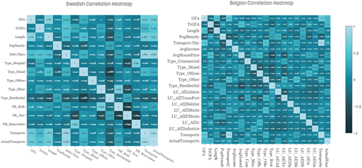
Multivariate data analysis was used to grasp complex data sets which require concurrent examination of all variables, thereby attempting to extract the underlying patterns in the data (Everitt and Dunn, 2001; Hair, 2009; Yates, 1987). The exploratory data analysis (EDA) aims to arrange data points and are typically designed for open-minded exploration with the goal to reveal otherwise hidden ranks, patterns and relationships (Komorowski et al., 2016; Morgenthaler, 2009). The methods used in EDA can be divided into two types: non graphical and graphical methods. The non-graphical methods consist of summarizing the data using summary statistics, such as calculating the mean, standard deviation or IQR. The EDA involved using scatter plots to visualize relationships between features and the number of transports. A correlation matrix was then created to identify linear relationships between feature pairs. Correlation coefficients can range from −1 to 1, where 1 indicates a strong positive correlation, −1 indicates a strong negative correlation, and 0 indicates no linear relationship. High or low correlations can provide insights into dependencies between variables, guiding further investigation or decision-making.

The next step comprises feature selection, a method of reducing the number of features to only those that are important for the prediction task. There are several ways to reduce the number of features. The main problem with using large feature sets is that some features may be redundant and do not add anything to the model. In addition, having too many features could lead to poor generalizability for the model (i.e. the model can fit the training data very well but is not able to predict on unseen data). In a recent publication, James et al. (2023) proposes three methods for linear model selection: subset selection, shrinkage, and dimension reduction. Subset selection involves finding a subset of the features that represents the data. On the other hand, shrinkage involves fitting a model with all the features and adding a regularization term that sets the irrelevant features to zero. Dimension reduction involves linear combinations of the features into principal components which captures the variance in the data set. As the aim of this paper is to investigate which combination of features can be used to predict construction transport demand, we will further investigate subset selection. James et al. (2023) propose best subset selection and stepwise selection when conducting feature selection. Best subset selection consists of three steps. The first step is to run a statistical/machine learning model, thus retrieving a base line. The second step is to run the model with all different combinations of features that contain exactly k features, where k ranges from 1 to the total number of features and is increased after every iteration. The R² and the Adjusted R² are then calculated for each different combination and the one with the largest R² is then picked as the best model for exactly k number of features. The model with the largest Adjusted R² is then picked as the best model among the k different models. On the other hand, stepwise selection does not try every different combination of features. Instead, it starts out by selecting the most important feature and keeps it for the next iteration. Then, every feature that is not included is tested in combination with the most important feature. The one with the best performance is then kept for the next iteration. This is done until we reach the total number of features. This is known as forward stepwise selection. This can also be done in reverse, also known as backward stepwise selection, where we start with all features and remove the least important feature at every iteration. One advantage of using stepwise selection compared with best subset selection is that the number of fitted models can be significantly lower for many features. The number of fitted models for best subset selection is equal to 2^p, where p is the number of features. On the other hand, the number of fitted models for stepwise selection is equal to $∑k=0p−1(p−k)=1+p(p+1)/2$ models (James et al., 2023).

We use stepwise selection to identify relevant features for predicting the number of transports for a construction project. Both forward and backward stepwise selection are used. The stepwise selection is implemented in Python 3.11 using the pandas, plotly, and scikit-learn packages. Only linear regression is considered in the stepwise selection. Three feature combinations, later referred to as tests, were performed for each dataset. The first test uses only the continuous features in the dataset, while the second test uses all features. The categorical features were coded using one-hot encoding. This means that each different value in the categorical features becomes a separate feature, for example, hospital projects become a binary feature. The third test also uses all the features, but the subtype is combined with the GFA. This creates different lines for each subtype, rather than just shifting the line up or down. Only the training set were used for the stepwise selection, due to the small amount of data. The performance of the models was then evaluated using the R² for each iteration of k. R² provides an explanation of the extent to which the model captures the variance in the data. This is measured on a scale ranging from 0 and 1, where 0 denotes that the model is not explaining more than the average of the response variable and 1 indicates that the model can capture the response variable perfectly (James et al., 2023). Therefore, it gives an initial understanding of how well the model captures the variance in the data and is thus included in the model assessment. The model with the highest R² is selected for each iteration and compared using the Adjusted R². This is because the Adjusted R² adds a penalty for the number of features, as the regular R² is likely to increase as more features are included. Thus, an unnecessary large number of features will only decrease the performance of the model. The model with the highest Adjusted R² is then selected along with its features. Other evaluation metrics were also considered, such as Akaike information criterion and Bayesian information criterion, but Adjusted R² was ultimately selected for its simplicity and similarity with R². The Root Mean Squared Error (RMSE) is also calculated to provide a more interpretable performance indicator. R², Adjusted R², and RMSE are each calculated according to Equation (1)–(3) respectively, where $yˆi$ is the predicted value, $yi$ is the actual value, $y¯$ is the mean value of the actual number of transports for the datasets, n is the number of construction projects, and p is the number of features considered.

To perform the predictive analysis for the number of transports for a construction project, three linear regression models and two decision tree models were used to test the effect of different models on the prediction performance. It is important to test several models as there is rarely one perfect model for a dataset. This is because of different models assume different structures within the data (Lones, 2021). It is also worth testing models with different degrees of flexibility and complexity (i.e. the ability to capture patterns in the data). The literature highlighted several models that have previously been used to predict freight demand with various degrees of complexity. The linear regression models considered OLS regression and ridge regression (RR). OLS tries to fit a linear regression line to all data by minimizing the sum of squares between data points and the regression line. These models are simple and should give a good baseline in terms of performance. However, OLS is very sensitive to outliers (Craven and Islam, 2011). RR is based on regularization and punishes large values of regression parameters to avoid overfitting. Regression models are trained on the data and the significance of the features are calculated (Cantoni and Ronchetti, 2001). In addition to linear regression, KNN and decision trees were also utilized. KNN fits features according to Euclidean distance, taking the average response of the K closest data points in the feature space as the prediction. KNN is a nonparametric model that does not assume a function for the prediction (Lindholm et al., 2022). Decision trees are interpretable models which divide the data into regions by minimizing the residuals within each region (Song and Lu, 2015). The regions are determined by finding tree splits that are minimizing the within-region residuals. However, regular decision tree models can suffer from poor accuracy (high bias) and can also be sensitive to changes in training data (high variance) compared to other models. Therefore, we used two more advanced versions: RFR and GBR, both of which have proven their use in sustainable urban development (Jun, 2021), and freight generation modeling (Khan and Machemehl, 2015). RFR uses bagging (resampling of data) and learns from a previously fitted tree along with excluding certain features to reduce the correlation between the fitted trees (Lindholm et al., 2022). GBR is an iterative model that attempts to minimize the residuals of the previous tree (James et al., 2023; Lindholm et al., 2022). The use of five different ML models allows for a robust comparative analysis of their effectiveness in this novel domain. Other more complex models, such as NN, were considered at this stage. NN can capture complex behavior in large data sets at the expense of interpretability. However, due to the limited amount of data available, the risk of overfitting with a neural network is very high (Lones, 2021) and was therefore not included. In the context of construction transport demand prediction, a model that overfits leads to low prediction errors for seen data and high prediction errors for unseen data, potentially assuming more deliveries than what occurs.

The data containing continuous values, such as GFA and average income, was normalized before final testing. Normalization is the process of rescaling the data to the same range as some features have different units. This can increase the performance of more complex models, like RFR and GBR (James et al., 2023; Lindholm et al., 2022). Examples of normalization techniques are min-max normalization and mean value of zero and unit variance. In our case, the data was normalized with a mean value of zero and a unit variance of one as it handles outliers better than min-max normalization (James et al., 2023). Another aspect that also affects performance is the choice of hyperparameters for KNN, RR, RFR, and GBR. Therefore, the hyperparameters were tuned before final testing. The hyperparameters were determined from the lowest RMSE value. This includes the number of neighbors k for KNN (ranging from 1 to 20) and the regularization parameter for RR. The maximum depth, the learning rate, and the number of estimators were tuned for RFR and GBR respectively.

Since the amount of data is limited, the models were trained using k-fold cross-validation (CV), partitioning the dataset into multiple subsets or folds (Fushiki, 2011). One fold is reserved as the test set, while the remaining k−1 folds collectively serve as the training set. In this study, the Swedish and Belgian data sets were each divided into five folds (k = 5). This process is repeated five times, ensuring that each fold acts as the test set exactly once. The model is trained on different combinations of training and test sets in each iteration, allowing for a comprehensive evaluation of its performance across various subsets of the data. K-fold CV helps mitigate issues related to overfitting or underfitting that may arise when using a single fixed training-test split. By averaging the performance metrics over multiple iterations, it provides a more robust estimate of the model’s accuracy and ensures a more reliable assessment of its ability to generalize to unseen data (Wong and Yeh, 2019). The performance of the model is evaluated by calculating the Root Mean Squared Error (RMSE) and R². The multivariate exploratory data analysis, feature importance, and prediction modeling were performed in Python 3.11 using the pandas, plotly, scikit-learn, and statsmodels packages. Pandas provides data management tools, plotly was used to visualize the data and results, while scikit-learn and statsmodels provided the decision tree and linear regression models.

This section presents the results in three subsections: (1) the results from the exploratory data analysis, (2) the feature selection and feature importance, and finally, (3) the models’ prediction performance.

For Sweden, the data from booking systems allowed for an accurate hourly overview of deliveries, presented in Figure 3. The distribution shows that the majority of deliveries take place in the early morning and are not equally distributed throughout the day. This is in line with findings from i.a. Sezer and Fredriksson (2020) and Brusselaers et al. (2024) where construction deliveries are overlapping with morning peak traffic.

Scatter plots showing the relation between GFA and number of transports are visualized in Figure 4. Overall, both the Belgian (A) and the Swedish (B) plots exhibit similar results, with slight variations with regards to the construction subtypes (hospital, residential, offices, commercial, mixed). Most noticeable are the plot scales, highlighting the different geographical context. Most notably are the very high number of transports required for hospital projects compared to their GFA (only present in the Swedish dataset), as illustrated by the red dots in frame B.

Beside the differences between the construction subtypes, also transport variations between different construction phases are noticeable, as presented in Figure 5. Construction sites were divided in four temporal phases where phase 1 covers 0–25% completion, phase 2: 25–50%, phase 3: 50–75% and phase 4: 75–100%. While construction activities can be overlapping across phases, these largely coincide with (1) the site preparation, ground works and construction of the load-bearing structure, (2) the framing and completion of the building structure, (3) the installation of services and interior works and (4) the moving-in and final clean-up (Åkerberg et al., 2024). Both contexts in Belgium and Sweden follow a similar pattern, where a higher number of transports per phase and per GFA is noticeable in phase 3 of a construction site, which is in line with findings of Sezer and Fredriksson (2020). Further results of the exploratory data analysis can be found in the  supplementary materials.

Three feature selection tests (FS) were conducted, of which the adjusted R² results are presented in Figure 6.

• (1)

  FS1 only considers continuous features, considering 5 features for Belgium (GFA, length, average income (AI), average house price (AHP) and population density (PD)), and 3 features for Sweden (GFA, length and population density). Overall results of the first test show that next to all features show relative importance and increasing the adjusted R² value. GFA is the most important feature no matter the method used, in both contexts, followed by length. For Belgium, the optimal number of features is reached by including all considered features, reaching an adjusted R² of 0.49. For Sweden, population density does not add significant importance, an optimal adjusted R² of 0,47 is reached considering GFA and length. Ultimately, the obtained results show that (1) adjusted R² are insufficiently good (R² ≤ 0) scoring worse than the average value, and, consequently, (2) that more features should be included in the analysis.

• (2)

  FS2 therefore considers all available features, incl. both continuous and categorical features, for Belgium (16) and Sweden (8). In both contexts, GFA remains the most important feature. Depending on the stepwise selection type, average income (AI), average house price (AHP), subtype and land use complete the list of important features, reaching an R² of 0.65, an adjusted R² 0.53 and an RMSE of 44, by combining 9 features. In Sweden, the hospital and mixed subtypes show to be determinants in relation to the number of transports. By combining 3 features, an R² of 0.82, adjusted R² of 0,81 and RMSE of 3,001 is reached. While better results are obtained compared to FS1, still high variances are noticeable between projects’ subtypes.

• (3)

  FS3 therefore considers all features but combines GFA and subtype. Hence, the model is run for each subtype, where a separate regression is calculated for each. Here, the model found a relationship between the combined specific subtype and the number of transports that is stronger than the normal GFA would be, with an R² of 0.75, adjusted R² of 0,67 and RMSE of 3,667 for Belgium, and an R² of 0.82, adjusted R² of 0,81 and RMSE of 3,001 for Sweden.

Overall GFA as standalone feature does not provide sufficient information to derive accurate construction site transport demand. However, the combination of GFA, subtype, average income, average house price, and to a lesser extent population density and environmental certification are highlighted as important features showing a relation with number of transports, especially in Belgium. Other features such as most land use types and length do not add significantly to the relation with number of transports. In Sweden, the combination of GFA and subtype provides the most positive results given the considered data and feature sets. Other features, such as population density, environmental certification and subtypes other than hospital or mixed, do not add significantly to the relation with number of transports. Further results of the feature selection tests can be found in the  supplementary materials.

Predictions were computed using the OLS, KNN, Ridge, GBR and RFR. The performance of the five models is calculated using R² and RMSE for both contexts, as presented in Figure 7. For each country’s data set, the respective selected features are used to perform predictive analyses. The central tendency is more pronounced in the results of the models using data from Sweden, where both the median value and the IQR are closer and more concentrated to 0, indicating fewer under- or overestimations for individual construction site transport demand predictions. Similar results are obtained in the context of Belgium, although the data observation spread is higher, indicating that results are more strongly under- or overestimating transport demand. In summary, the models’ performance when predicting transport demand for individual construction sites is poor, due to relatively strong over- and underestimated predicted values.

Conclusively, it is very difficult to accurately predict the number of transports to a construction project. The machine learning models did not produce sufficiently good results as there is a large variance in the data for both sets. The results show that the machine learning models can capture the general structure within the data. However, it struggles to predict unseen data. From the final results, we can observe an improvement in test error rates for all tests compared with using all available features. This can be explained by excluding irrelevant features from the model. Therefore, we see that the feature selection worked in including only relevant features, but better data is needed for further analysis. It can be concluded that construction transport demand is influenced by a wide array of context-specific factors, many of which are difficult to quantify or may not be fully captured in the available data. Unlike traditional freight models that rely on aggregate economic indicators, this study’s approach sought to integrate construction-specific project data, which introduces variability that standard models struggle to encapsulate.

Urban construction transport is understudied because its demand predictors remain unexamined. This proof-of-concept study reveals the complex factors affecting demand and outlines key data requirements for future research. Current urban freight models struggle with scarce, fragmented, and distributed data sources, leading to highly aggregated or oversimplified representations of construction transport demand. This study addresses this by leveraging diverse, construction-specific data sources that have not been systematically integrated into urban transport demand models before, providing an initial proof-of-concept (POC) to demonstrate how a data-driven, ML-based approach can enhance the features to consider in forecasting construction transport demand. While the models show poor predictive power, their ability to extract meaningful patterns from complex construction data remains valuable. This study integrates construction-specific features missing from conventional urban freight models. It benefits urban planners, freight modelers, construction contractors, and environmental certification organizations by enabling context-aware demand estimates that better align with real-world construction logistics and sustainability data needs.

One of the main findings of this study is that GFA is the most important feature for both the Swedish and Belgian data sets. This means that larger construction projects tend to require more transports than smaller ones, which is intuitive and in line with previous studies (Brusselaers et al., 2023a, b; Sezer and Fredriksson, 2021). However, GFA alone does not explain the whole variation in the number of transports, as there is still a lot of unexplained variance in the data. This could be due to (1) missing features in the data set that could influence transport demand, (2) project complexity, design, material choice, or construction method, or even (3) differences in how data for the number of transports are collected or reported by different sources (such as booking systems or on-board units). Alternatively, it could be due to a large randomness in the number of transports for different construction sites, depending on factors that are not easily measured or controlled such as production planning and purchasing routines. While the study’s data from Sweden and Belgium show broader applicability, urban construction transport is shaped by local policies, regulations, and infrastructure. Thus, generalizing these findings requires caution and recognition of the data’s limitations.

A main outcome of this study is the ability to interpret the lack of available data. First, the scope of this study was limited to commonly available project- and context-related features. Given more data, future research could develop better machine learning models considering additional features. This problem is to be traced back to the low digitalization level of the industry and to change would require another view of data in the construction industry; a view where data has a value and not only as summarized value to be put into evaluations and accountings. Here both developers and environmental certification organizations have a role to play, by also asking for standardized digitalized data sets and not only final numbers. If the problem of lack of data quantity and quality is not taken seriously, there is a risk that new actors might push the existing structures and with data as a base provide new types of services. This can already be seen taking place on the construction logistics scene, where actors such as material providers and rental companies are taking over site planning and logistics management. More specifically, the utilized logistic setup might be a predictor in forecasting transport demand, in turn offering insight into potential future services and volumes to consolidate material deliveries across multiple sites.

The study shows that a project’s number of transports have a relation with the combination of GFA and project subtype. It is also shown that environmentally certified projects show a slight negative correlation with the number of transports, suggesting that higher environmental building goals have a slight positive effect on transport planning, a finding which is in line with Sezer and Fredriksson (2021) and Fufa et al. (2019). It also must be noted that the environmentally certified projects are more prominent in Sweden, thereby leading to a potential bias in the data set for this variable. There are several different project-related variables that can explain transport demand discrepancies such as regional (construction) transport regulations and instruments (Bø et al., 2021; Janné and Fredriksson, 2019), utilized construction logistic setups (Janné, 2020; Janné and Rudberg, 2017) or the number of suppliers (Hjorth, 2023), which were not accessible as part of this study. To broaden the perspective and include considerations construction merchants or contractors’ data and understanding of what drives transport demand in projects would also provide opportunities for deepened analysis (Hjorth, 2023). Analyzing data from multiple projects reveals how delivery numbers correlate with project features, offering insights into transport demand variance. This can guide strategies to reduce transport volumes, improve logistics efficiency and sustainability, and help third-party logistics tailor setups to project demands (Eriksson and Olsson, 2022). More specifically, practical applications allowing to better consolidate material flows entering a city for many construction sites might be envisioned if construction transport predictions are rendered accurately, hence offering benefits for both city and traffic planners, and contractors to reduce the amount of vehicle movements to site.

The negative correlation between population density and the number of transports could be explained by prior research in construction logistics. These has repeatedly investigated large and prestigious projects (Bengtsson-Hedborg et al., 2017; Ekeskär and Rudberg, 2016; Janné and Fredriksson, 2019; Sundquist et al., 2018) and the common thread is that a significant share of construction transport research has been focusing on urban, hence more densely populated, areas. The more prestigious and the more important and more spatial restrictions a project has, which is usually the question of densely populated are, the more efforts seem to be put into efficiently organize transports to and from these areas, which can explain this negative correlation. Other features such as land use types do not significantly contribute to the relation with transport demand. Also, the duration of a site was found not to contribute significantly. An explanation for this could be that a project’s GFA, cost and duration are highly correlated among themselves (Hjorth, 2023), and that the model favored GFA as most appropriate feature without the length of a project to marginally improve the results.

Except from data quantity, also higher-quality data should be sought, as the models for the data sets used are suffering from high variance and high bias. Data sources such as booking systems or on-board units were not primarily designed to run analyses as presented in this work, these are very much focused on tracking and tracing the transport per se. Further data collection will help to reduce the variance, and the consideration of additional features could be added to reduce the bias. The present development of modern construction projects, which increasingly integrate diverse data sources such as economic indicators, geospatial data, real-time sensor information, will enable this. The combination of data sources is important as the results show that standalone project-related variables (such as gross floor area (GFA)) do not provide sufficient information to derive accurate construction site transport demand. This study suggests that future studies utilize ML algorithms to incorporate these higher-dimensional inputs, even when each input’s exact causal contribution is more difficult to interpret. For further interpretability, future research could also explore the use of hybrid ML-econometrics models (Pérez-Pons et al., 2022). Patterns emerge when combining context- and project-related features, but this feature offers limited benefit compared to others regarding transport numbers.

Further research is required to put the results obtained in this study in context with future analyses using better data in terms of quality and quantity. Note that in the feature selection stage, the entire training set was used and not divided into a CV set. This was to allow the model to train on the entire data set because of the limited amount of data. A limitation is that the models’ performance when predicting transport demand for individual construction sites is poor, due to relatively strong over- and underestimated predicted values, missing features and noisy data. Given stronger datasets, Naoui et al. (2021) demonstrate how deep learning can be scaled and distributed for real-time urban data analysis, which could be adapted to predict urban construction transport demand. Their approach to processing big data in urban settings aligns with transport modeling, where multiple real-time data sources (such as GPS tracking or traffic sensors) must be analyzed efficiently.

The study emphasizes the need for standardized data collection in the construction sector, which could inform policies related to urban planning, transport logistics, and environmental regulations. Linking construction transport with urban and traffic planning has potentials for reducing traffic congestion and improving city logistics efficiency. This study therefore raises the question if more accurate results can be obtained when looking at the prediction of a context (or city) as a whole, rather than individual construction sites. While ML has been applied to freight transport modeling in general, its application in construction logistics forecasting remains scarce. Our study bridges this gap by introducing ML-based modeling specifically tailored to construction transport demand, which is characterized by project-specific variations, temporal dependencies, and urban planning constraints. In this sense, this study highlights the potential of machine learning for transport and urban planning purposes and the increasing importance of applying ML to handle the complexity and variability of urban construction logistics.

Given the potential practical and managerial implications data-driven methods can have, this study underscores the importance of deploying such modeling techniques to investigate the relation between construction transport planning, urban planning and traffic planning, as shown in Figure 8. In turn, this can then be used to predictively model construction transport-related disturbances and improve transport efficiency, as suggested by prior research on the topic (Brusselaers et al., 2024; Brusselaers et al., 2023a, b; Fredriksson et al., 2022).

Improved data collection methods, potentially led by environmental certification organizations, could help embed sustainability principles into construction logistics. From a policy standpoint, the results point to the importance of standardized data (Puslat et al., 2024) across the construction sector, guiding future regulations on urban development, transport logistics, and environmental safeguards. This study emphasizes to prioritize the collection of specific features, in particular GFA, project subtypes, average household income, average house prices, and to a lesser extent environmental certification and population density, features which show the highest link with transport demand. In turn, by linking construction transport to urban and traffic planning, this study also opens pathways for mitigating congestion and enhancing overall city logistics efficiency. These findings offer practical implications for urban planners, who can refine zoning policies and land use strategies by considering the nuanced relationships between gross floor area (GFA) and specific building subtypes. Moreover, by leveraging exploratory data analysis results, stakeholders can implement targeted interventions to alleviate congestion and enhance urban mobility, such as scheduling commercial deliveries outside peak traffic hours (Mommens et al., 2018; Saleh et al., 2022). Finally, from a societal perspective, environmentally certified projects appear to slightly reduce transport demand, reinforcing urban sustainability efforts. With better data-driven decision-making and enhanced stakeholder collaboration (Fredriksson and Huge-Brodin, 2022; Huang et al., 2025), such approaches could further decrease emissions and strengthen the quality of life in growing urban centers (Brusselaers et al., 2023a, b, 2024; Fredriksson et al., 2022).

This study demonstrates the potential of ML in a domain where traditional methods fall short, showing the role of construction-specific and contextual data in transport demand predictions in a proof-of-concept (POC). Thereby, it aimed to answer the research question if urban construction site transport demand can be predicted with commonly available project and/or context-related data. To this end, a multivariate exploratory data analysis was performed using linear and decision-tree regression models. This study found that Gross Floor Area (GFA) is the most important factor for predicting transport numbers in both Swedish and Belgian datasets, aligning with earlier research. While larger construction projects require more transports, GFA alone doesn’t account for all variations, which may be due to missing data like project complexity or differences in data collection. However, patterns are noticeable when combining multiple context- and project-related features. GFA, project subtypes, average household income, average house prices, and to a lesser extent environmental certification and population density show the highest link with transport demand. In this regard, the machine learning model can capture the general structure within the data. However, it needs to be emphasized that accurately predicting the number of transports to a construction project remains difficult, as the machine learning models struggle to predict unseen data and in producing sufficiently good results given the large variance in the data sets. This may stem from various sources of uncertainty in the data, such as project characteristics that affect transport demand but are not captured by the features in the available data sets, discrepancies in how the transport data are collected or reported by different methods, or a high degree of variability in the transport demand for different construction sites, depending on factors that are hard to measure or control. This study therefore highlights the need for higher-quality data collection in future research, and suggests that better data collection practices -which do not require much effort from various actors- and improved machine learning models could enhance transport demand forecasting. This study should thus been seen as an initial step, suggesting that integrating additional and identified relevant data sources could improve predictive performance, underscoring the importance of data augmentation strategies such as the integration of real-time IoT sensor data for dynamic model updates, and the viability of ML for construction transport demand prediction. Future data-driven methods could put in comparison the results obtained in this study, and further explore the relationship between construction transport planning, urban planning, and traffic planning to improve transport efficiency.

This study did not involve any human participants or animals.

Table A1