Real-time trajectory tracking and stabilization of quadrotors using deep Koopman-based model predictive control

Quadrotor aerial robots, with their lightweight design and agile six-degree-of-freedom motion, have emerged as highly versatile platforms for research and practical applications [1, 2]. Their ability to perform rapid maneuvers, hover with precision and operate in constrained environments makes them suitable for diverse tasks such as aerial surveillance [3], package delivery [4], environmental monitoring [5] and search-and-rescue missions [6]. Furthermore, quadrotors are widely used as testbeds for advanced control strategies and embodied intelligence [7]. However, achieving reliable and high-performance control remains a challenge due to the strongly nonlinear dynamics of quadrotor flight, the tight coupling between translational and rotational states and the sensitivity to disturbances such as wind gusts and payload variations. These factors make precise modeling and control design difficult when relying solely on traditional analytical approaches [8–10].

To tackle these challenges, two dominant control methodologies have emerged in quadrotor research: model-based control and learning-based control [11]. Model-based strategies often employ simplified dynamics, such as linearization around hover conditions using Linear Quadratic Regulator (LQR) or feedback linearization techniques, to effectively approximate the quadrotor's behavior under specific assumptions [7, 12]. While these approaches offer structured frameworks for control design, their reliance on simplifying assumptions can lead to model-plant mismatches and suboptimal performance when faced with real-world disturbances or agile maneuvers [13].

To overcome the limitations of traditional model-based control, modern research has increasingly turned to learning-based strategies that leverage deep learning methods to better capture complex quadrotor dynamics and couplings [14]. One promising approach involves learning inverse dynamics: neural networks trained to map desired trajectories directly to actuator commands, simplifying controller implementation and enabling agile flight in challenging scenarios [15, 16]. However, the inherently underactuated nature of quadrotors and the possibility of multiple valid inverse mappings introduce challenges for these methods, potentially affecting generalization and stability.

Another avenue explored is reinforcement learning (RL) [17], where control policies are trained in simulation, either model-free or with learned models, and then deployed on real quadrotors [18]. While RL offers the flexibility to discover effective control strategies through experience, its deployment is often hindered by the sim-to-real gap. Transfers from simulation to real-world quadrotors can falter unless substantial domain randomization, real-world adaptation or robust policy learning techniques are applied [19].

To overcome the difficulties of modeling forward dynamics in quadrotor systems, Koopman operator–based methods have gained momentum, offering a compelling strategy for control design [20–22]. By embedding the nonlinear dynamics into a lifted space where the system evolves linearly, these approaches enable the deployment of efficient linear control techniques. However, a critical challenge lies in defining appropriate lifting (observable) functions; insufficient or suboptimal choices can introduce substantial modeling errors, negatively impacting prediction fidelity and controller effectiveness [23, 24].

While Koopman operator theory has recently gained traction for unmanned aerial vehicle (UAV) modeling and control, most existing studies rely on linear or shallow lifting architectures. These approaches often struggle to capture the strong nonlinearities inherent in quadrotor dynamics – particularly during high-rate or aggressive maneuvers – leading to reduced predictive fidelity and suboptimal closed-loop performance. To address this gap, we introduce a deep Koopman-based model predictive control (DK-MPC) framework that employs deep neural networks (DNNs) to automatically learn high-dimensional nonlinear embeddings. By achieving a more expressive, globally linearized representation of quadrotor dynamics, our method enables real-time optimization of control inputs. The resulting framework provides a scalable, data-driven alternative to conventional lifting methods, ensuring high-precision trajectory tracking and robust performance on physical quadrotor platforms.

The proposed Koopman-based approach belongs to a broader class of strategies aimed at nonlinear-to-linear conversion, most notably sharing conceptual goals with differential flatness. While both paradigms leverage linear structures to simplify controller design, they differ fundamentally in their mathematical foundations and implementation trade-offs. Quadrotors are well known to be differentially flat, meaning their states x and inputs u can be mapped to a set of flat outputs σ = [x, y, z, ψ]^T and their finite derivatives. As highlighted by Li et al. [25], leveraging this property allows for exact linearization without the need for small-angle approximations, providing a rigorous framework for flatness-based model predictive control (MPC). However, while flatness provides an elegant analytical mapping, it typically relies on a precise nominal model and can struggle to account for unmodeled aerodynamic effects or complex ground-effect dynamics.

In contrast, Koopman-based methods utilize data-driven spectral lifting to approximate the nonlinear flight dynamics in a high-dimensional linear space. While differential flatness offers exactness within the constraints of the analytical model, Koopman operators provide a more flexible framework for capturing non-conservative forces or structural uncertainties that lack a simple flat representation. Thus, the choice between these methods involves a trade-off between the structural requirements of analytical flatness and the global, yet approximate, flexibility of data-driven lifting.

Numerical simulation experiments on a data-driven quadrotor model validate the effectiveness of the proposed DK-MPC framework. The results show that DK-MPC achieves highly accurate control performance, with clear improvements over conventional nonlinear control strategies. These outcomes highlight the potential of DK-MPC for future quadrotor applications, particularly in scenarios requiring precise trajectory tracking and robustness against dynamic variations [20]. Moreover, as a data-driven method, DK-MPC can be easily adapted to different quadrotor platforms, providing a flexible and scalable solution for advanced aerial robotics.

The remainder of this paper is organized as follows: Section 2 presents the development of the proposed DK-MPC framework, highlighting the integration of the deep Koopman operator with MPC. Section 3 reports the results of numerical simulation experiments, demonstrating the effectiveness of DK-MPC in enabling the quadrotor to accurately track reference trajectories while respecting system constraints. Finally, Section 4 concludes the paper with a summary of key findings and outlines directions for future research.

This section presents a comprehensive overview of the methodology behind the proposed DK-MPC approach, tailored to tackle the control complexities of quadrotors. It begins with an introduction to the overall architecture, followed by an explanation of the Koopman operator's formulation and learning process in high-dimensional settings, and concludes with the integration of the learned Koopman model into the MPC framework for control implementation.

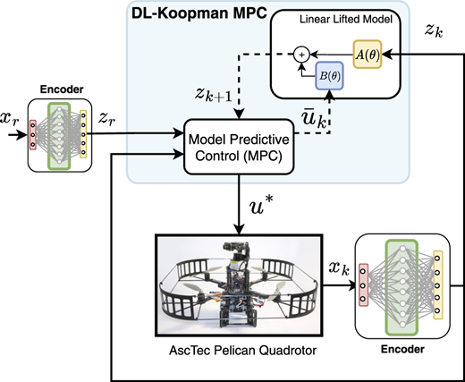
Figure 1 depicts the structure of the proposed DK-MPC approach. It utilizes a deep learning-based Koopman operator to create a globally linear, time-invariant representation of the nonlinear quadrotor system by mapping the original state space into a higher-dimensional latent space. During each control cycle, the deep Koopman encoder maps the reference state x_ref into its corresponding high-dimensional latent representation. Simultaneously, the current state x, obtained from the quadrotor, is encoded into the same latent space. Within this transformed space, an MPC algorithm optimizes a quadratic cost function based on the latent states z and z_ref over a finite prediction horizon H, thereby producing the optimal control input u* to follow the reference trajectory.

Having a linear system representation in the latent space is essential because it enables the use of efficient quadratic programming solvers within the MPC framework. For nonlinear dynamics, the corresponding NMPC problem typically leads to a non-convex optimization that is computationally expensive and may fail to converge in real time, especially for fast systems such as quadrotors. By contrast, the Koopman-based linearization ensures that the MPC optimization remains convex and tractable, allowing control inputs to be computed within strict timing constraints while still capturing the essential nonlinear behavior of the original system. This balance between fidelity and computational efficiency is what makes the proposed DK-MPC framework suitable for real-time quadrotor control.

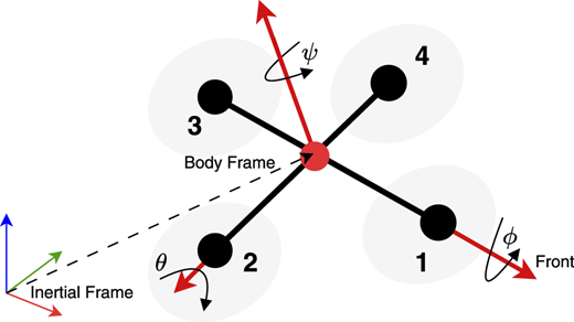
We examine a discrete-time nonlinear system governed by a function f, which describes the evolution of the state in the quadrotor. In this context, x_k = [x, y, z, ϕ, θ, ψ]^T denotes the system's state at time step k, representing the quadrotor's position and Euler angles, i.e. roll, pitch and yaw, respectively (Figure 2), and $uk∈R4$ represents the corresponding commanded motor speeds, such that:

Due to the inherent complexity and nonlinearity of f, directly designing a control strategy can be challenging. To address this, we apply the Koopman operator framework, which operates in a transformed (lifted) space defined by a mapping function ϕ. This function lifts the original nonlinear system into a higher-dimensional space where its behavior becomes approximately linear:

The effectiveness of this linear approximation relies heavily on the choice of the lifting function ϕ. In this study, we adopt a deep learning-based method to learn ϕ enabling us to model the complex nonlinear dynamics typical of quadrotors.

Extending the Koopman operator framework, the lifting function ϕ(x, u) is separated into two components: one dependent on the state, ϕ_x(x), and the other on the input, ϕ_u(u), such that:

This decomposition enables the system dynamics to be expressed in a control-affine form through matrix operations:

From this, the evolution of the lifted state can be written as:

Consistent with simplifications proposed in earlier studies [26, 27], the input lifting function ϕ_u(u) is directly represented by the control input u. Defining K_xx = A, K_xu = B and ϕ_x(x_k) = z_k, the dynamics simplify to a globally linear form:

This transformation yields a linear state space model that not only facilitates controller synthesis but also effectively approximates the overall behavior of the original nonlinear quadrotor system.

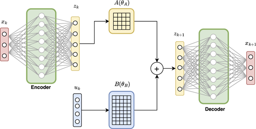
This subsection outlines the deep learning strategy employed to estimate the Koopman operator and its associated lifting and inverse functions. As depicted in Figure 3, the method is based on a deep auto-encoder architecture designed to learn the forward mapping ϕ(θ) and its inverse ϕ(θ)⁻¹. The auto-encoder comprises two primary components: an encoder and a decoder. The encoder ϕ(θ), implemented using a multi-layer perceptron (MLP), lifts the system's original state into a higher-dimensional latent space, where the system dynamics become approximately linear. Conversely, the decoder ϕ(θ)⁻¹ reconstructs the original state from this latent representation. Although alternative architectures such as convolutional neural networks or recurrent neural networks could also be promising for capturing spatial or temporal correlations in the data, the MLP was chosen for its simplicity, general approximation capability and efficiency in training on tabular state-action datasets such as those considered in this work.

To model the system's linear behavior in the latent space, two additional single-layer MLPs are employed to approximate the matrices A and B from Equation (6). These networks are designed without biases or activation functions, enabling them to function as straightforward linear transformations. This structure ensures that the learned latent dynamics remain consistent with the theoretical assumptions of the Koopman framework.

Reconstruction loss: To accurately model the relationship between the original and latent state representations, a reconstruction loss is defined using the L₂ norm. This loss ensures that the auto-encoder learns to map states to and from the latent space with minimal error:

Linear dynamics loss: To identify the linear operator A and the control matrix B, we define a dynamics loss that encourages the latent state transitions to follow a linear model structure. This objective penalizes deviations from the expected linear behavior in the latent space:

Stability loss: To promote stability in the learned Koopman operator A, we introduce a stability loss that penalizes cases where the spectral radius exceeds 1. Specifically, we compute the spectral radius ρ(A) as the maximum absolute eigenvalue of A and apply a rectified linear unit-based penalty to constrain it within the unit circle:

This loss term helps ensure the linear dynamics model remains stable by discouraging eigenvalues with magnitudes greater than one.

Total loss function: The final objective, as shown in Equation (10), is expressed as a weighted sum of the reconstruction loss, linear dynamics loss, stability loss, along with an L₂ regularization term to the model weights W to reduce overfitting [28]:

This integrated framework supports end-to-end learning of the Koopman-based model by jointly training the linear operator A, the control-affine matrix B and the lifting function ϕ. Consequently, it enables effective modeling and control of the nonlinear dynamics inherent in quadrotor systems.

Once the Koopman operator has been learned, we employ MPC to regulate the nonlinear behavior of the quadrotor. MPC is particularly well suited for systems with constraints and excels in optimizing control trajectories by predicting future system evolution [16]. Utilizing the linear system representation obtained via the Koopman framework, we can formulate an MPC scheme that is both efficient and effective.

The controller solves an optimization problem to compute an optimal sequence of control actions $uˆt:t+H*$ over a finite prediction horizon $H∈N$⁠. The cost function penalizes both the deviation from the reference trajectory in the lifted space and the magnitude of the control inputs:

Here, $Qˆ∈Rn×n$ and $Rˆ∈Rm×m$ are positive semi-definite weighting matrices that penalize state tracking error and control effort, respectively. The variables u_min and u_max define the allowable range for the control inputs, while n denotes the dimension of the latent (lifted) state space. At each control timestep, we encode the current system state x_t and future reference states $xt:t+Href$ into the latent space, yielding $zˆt$ and $zˆt:t+Href$⁠. Solving the optimization problem in Equation (11) produces an optimal control sequence, from which only the first control action $uˆt*$ is applied to the system. This process is repeated iteratively until convergence is achieved.

This section outlines the methodology for data preparation and the training procedure for the proposed model. We then deploy the DK-MPC controller to manage the motion of the quadrotor simulated using the system dynamics of equations depicted in Reference [29]. To validate the effectiveness of the proposed approach, we conduct three experimental scenarios: a path-following task, a moving target tracking task and a complex helical trajectory tracking task. The first experiment highlights the precision and fast dynamic response achieved by DK-MPC; the second illustrates its capability to adapt to dynamic conditions, while the third assesses the responsiveness of the control system to handle complex trajectories, indicating its potential for real-world deployment in responsive control applications.

To evaluate the proposed data-driven DK-MPC strategy in a dynamic aerial platform, we employ the dataset of the AscTec Pelican quadrotor, a research-grade UAV known for its modularity and robust performance. The quadrotor features a rigid carbon-fiber frame with a diagonal motor-to-motor span of approximately 85 cm and a total weight of around 1.6 kg, including battery and onboard electronics. It is powered by four brushless direct current motors equipped with fixed-pitch propellers and is capable of both high-thrust maneuvers and stable hovering.

The Pelican is equipped with an onboard computer running a real-time operating system, supporting integration with Robot Operating System (ROS) for high-level control and sensor fusion. It includes an inertial measurement unit, barometer and global positioning system module for autonomous navigation and offers payload options for additional sensors or manipulators. The platform's flexibility and open software interface make it ideal for implementing and validating advanced control algorithms, including the proposed DK-MPC framework.

For training and evaluating the proposed DK-MPC framework, we utilize the publicly available Pelican Dataset provided by the WaveLab group [29, 30]. This dataset was collected using the AscTec Pelican quadrotor in a controlled indoor environment equipped with a motion capture system. The dataset includes time-series recordings of the quadrotor's state and control inputs across various flight maneuvers.

Specifically, the dataset contains 35 different flights of measurements such as position, velocity, acceleration, orientation (quaternions), angular rates and motor commands, all sampled at 100 Hz. These high-fidelity recordings offer a comprehensive representation of the quadrotor's dynamic behavior and are well suited for learning both the lifting functions and the Koopman operator used in the DK-MPC framework.

To ensure robust training, we preprocess the dataset by segmenting it into input-output pairs (x_k, u_k, x_k+1), normalizing each feature and partitioning the data into training and validation sets. The richness and quality of this dataset make it ideal for modeling complex nonlinear dynamics in aerial robotics.

To facilitate robust learning, the dataset was divided into three subsets: training, validation and testing. Prior to training, all input features were normalized using the min-max scaling approach [31], which linearly transforms each feature to the range [−1, 1]. This normalization improves convergence and maintains consistency throughout the training process. The transformation is defined by:

This preprocessing step ensures that all features contribute proportionally during optimization, preventing dominance by features with larger numerical ranges [32].

The hyperparameters employed for training the proposed architecture are listed in Table 1. These were carefully selected to achieve a balance between model accuracy and training stability and were tuned through empirical testing and validation performance.

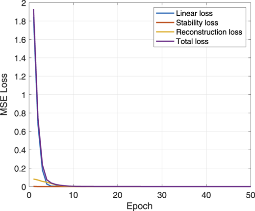
To evaluate the learning behavior of the proposed DK-MPC framework, we monitored the evolution of various loss components during training, as shown in Figure 4. The plot illustrates the convergence of the linear dynamics loss, reconstruction loss, stability loss and the total loss over 50 epochs. All losses exhibit a rapid decline within the first 10 epochs, stabilizing at near-zero values, which indicates fast convergence and training stability. The smooth decrease in the total loss suggests that the model effectively learns a Koopman-consistent latent representation, simultaneously satisfying reconstruction accuracy and spectral radius constraints. This behavior confirms the effectiveness of the loss design in guiding the model toward a stable and accurate linear approximation of the nonlinear system dynamics.

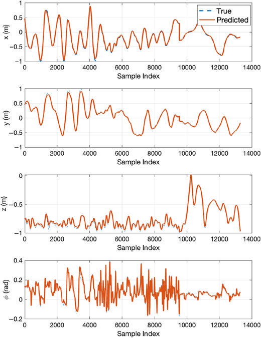
To evaluate the prediction accuracy of the learned Koopman-based model, we assess its one-step-ahead forecasting performance by comparing the predicted next state x_k+1 with the ground-truth test data across multiple state dimensions, including position (x, y, z) and roll angle (ϕ), as illustrated in Figure 5. The model's predictions (orange) closely match the true states (blue dashed lines), demonstrating its ability to reliably estimate x_k+1 from the current state-input pair (x_k, u_k). This strong agreement across all state channels indicates that the learned lifted linear representation is sufficiently expressive to capture the essential nonlinear dynamics of the quadrotor. These results confirm the suitability of the Koopman framework for accurate next-state prediction and support its effectiveness as a foundation for data-driven control design in complex dynamical systems.

To determine the appropriate size of the Koopman latent space, we conducted a sensitivity analysis by evaluating latent dimensions of 4, 6, 8, 12 and 16 against the prediction accuracy and the computation time, including the complete online control pipeline. The results, summarized in Table 2, show a clear trade-off between model accuracy and computational performance. Lower-dimensional embeddings (4 and 6) led to under-expressive representations, achieving average R² scores of only 71.32% and 86.13%, respectively. Increasing the latent dimension to 8 yielded a substantial improvement, achieving 99.45% prediction accuracy while maintaining a low computation time of 0.008 s per control step. Higher dimensions (12 and 16) offered only marginal gains in accuracy (up to 99.57%) but came with increased computational cost. Based on this trade-off, a latent dimension of 8 was selected as the optimal balance between model expressiveness and real-time feasibility for DK-MPC.

For a fair and transparent comparison with the proposed Koopman-based predictive controller, a conventional nonlinear MPC (NMPC) baseline was implemented using the full dynamic model of the quadrotor in DK-MPC. The NMPC formulation incorporated the system states for position (x, y, z), linear velocities, Euler angles and angular rates. Motor thrusts were represented through nonlinear actuator maps using the constants b_i and k_i, where each rotor force was modeled as $fi=(ui2+bi)/ki$⁠, thus capturing the nonlinearities inherent in quadrotor actuation. Physical parameters, including the arm length l = 0.2 m and drag constant d = 0.02, were embedded directly within the dynamic equations to ensure accurate prediction as indicated in Appendix A. The controller was solved using the default DK-MPC nonlinear optimizer with a single-shooting approach and a discretization consistent with the simulation step of 0.05 s. In the NMPC, the weighting matrices have been chosen to be Q = Diag([100, 100, 100, 10]) and R = Diag([0.001, 0.001, 0.001, 0.001]). The NMPC utilizes the dynamic position and rotation model alongside the quadrotor parameters depicted in Ref. [29] as the MPC prediction model.

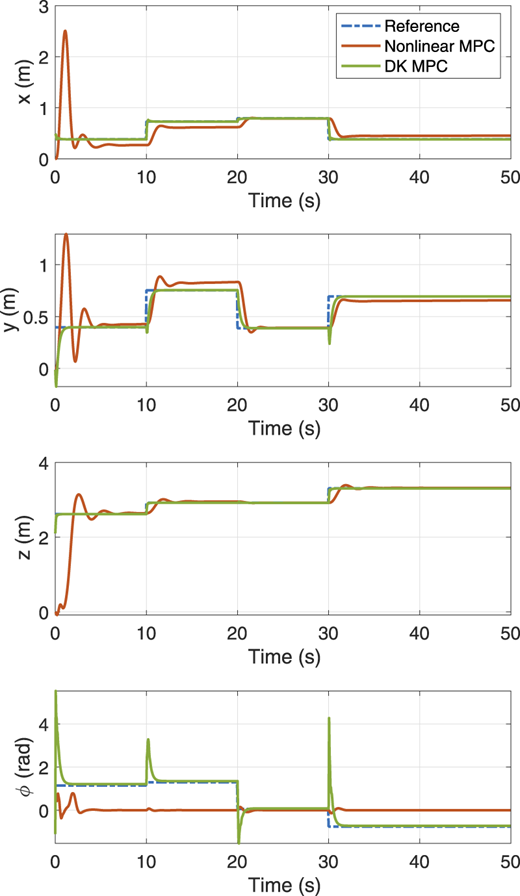
In the point stabilization experiment, the performance of DK-MPC is evaluated against a conventional NMPC with the same prediction horizon H across stepwise changes in target states. As shown in Figure 6, the DK-MPC controller demonstrates superior tracking accuracy and stability across all state dimensions. It responds quickly to abrupt changes in reference positions (x, y and z) and orientation (ϕ), with minimal overshoot and short settling time.

In contrast, the NMPC exhibits noticeable oscillations, slower convergence and greater steady-state error – particularly in the rotational dynamics. These results validate the capability of the learned Koopman-based linear representation to generalize well to unseen reference inputs, ensuring robust and efficient control in point-to-point tasks. The effectiveness of DK-MPC in handling sharp transitions also highlights its potential for real-time applications in agile and dynamic environments.

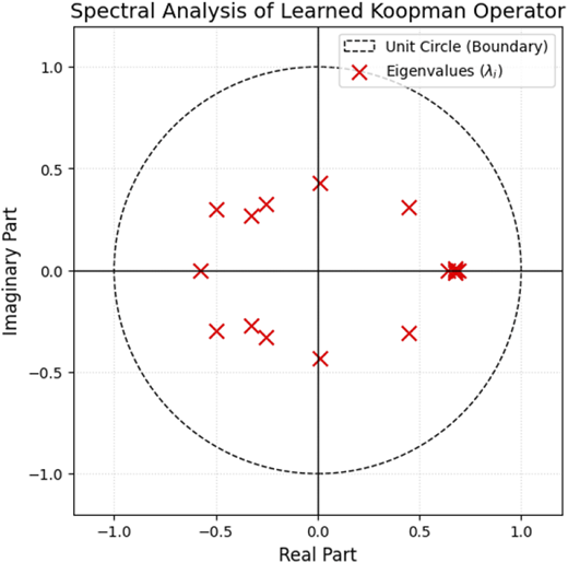
To rigorously assess the stability of the proposed DK-MPC framework, we analyze the spectral properties of the learned discrete-time Koopman transition matrix, denoted as $A∈RN×N$⁠. In this data-driven linear representation, the autonomous evolution of the lifted state z_k is governed by the linear relation z_k+1 = Az_k.

According to discrete-time control theory, the global stability of the equilibrium point is determined by the eigenvalues λ_i of the matrix A. The system is considered Lyapunov stable if all eigenvalues lie within the unit circle in the complex z-plane:

Figure 7 illustrates the eigenvalue distribution derived from our trained model. The results show that the eigenvalues are strictly contained within the unit circle (|λ_i| < 1) or reside at the marginal stability point (1, 0). The poles at (1, 0) correspond to the physical integrators of the quadrotor system (e.g. global position coordinates x, y, z), while the remaining poles, associated with the DNN embeddings, are strictly dissipative.

This spectral distribution provides a formal guarantee that the learned nonlinear embeddings do not introduce divergent modes. Consequently, the DK-MPC optimizer operates on a stable linear manifold, ensuring that the predicted trajectories remain bounded over the prediction horizon H_p.

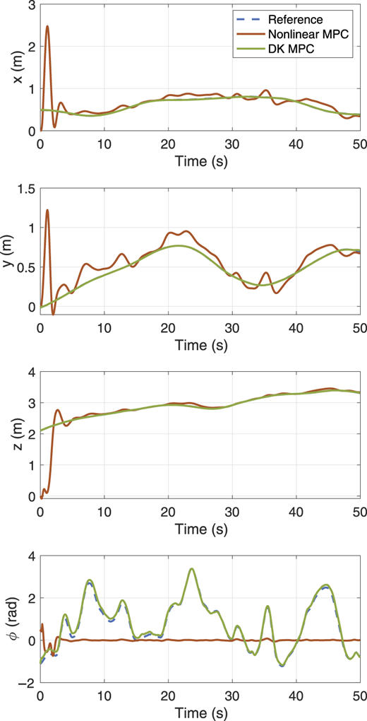
In the trajectory tracking experiment, the DK-MPC is further evaluated in a continuous motion scenario where the reference path evolves smoothly over time. As illustrated in Figure 8, DK-MPC consistently outperforms the baseline NMPC across all translational (x, y, z) and rotational (ϕ) states with the same prediction horizon H. The DK-MPC controller closely follows the reference trajectory with reduced tracking error and smoother control responses, while the NMPC exhibits lagging behavior and higher deviation, particularly during transitions and changes in trajectory curvature. These observations emphasize the effectiveness of the Koopman-based linear model in capturing global dynamics, allowing the controller to anticipate and adjust to trajectory changes more efficiently. The results affirm that DK-MPC not only achieves high tracking accuracy but also maintains stability and robustness during dynamic flight tasks.

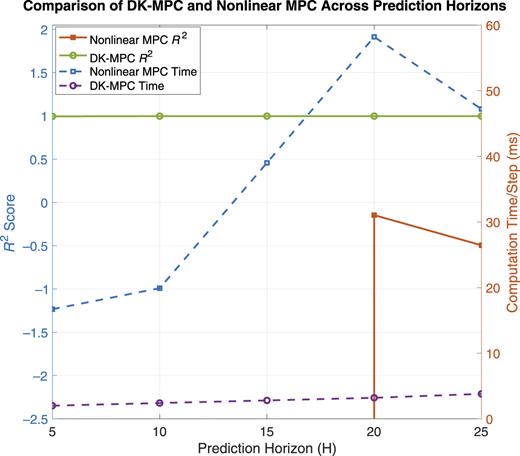
To further evaluate the performance and scalability of the controllers for real-time applications, we analyze how both DK-MPC and NMPC behave across varying prediction horizon lengths. As illustrated in Figure 9, DK-MPC consistently achieves high R² scores above 0.99 across all horizons, demonstrating robust prediction accuracy and reliable model generalization. In contrast, the NMPC shows extremely poor accuracy for shorter horizons (H = 5, 10 and 15), with significantly negative R² values, indicating divergence from the reference trajectory. Only at longer horizons (H = 20 and 25) does it begin to exhibit modest improvement.

On the computational side, DK-MPC maintains a low and stable control time below 5 ms per step regardless of horizon length, highlighting its suitability for real-time applications. NMPC, however, shows a steep increase in computational cost, reaching nearly 60 ms at H = 20. These results underscore the advantage of DK-MPC in achieving accurate control with minimal computational overhead, especially when scalability and fast response are critical in embedded or onboard systems.

The helical trajectory was chosen as a benchmark task because it simultaneously excites both the translational and rotational dynamics of the quadrotor while requiring continuous changes in altitude, heading and lateral position. Such a trajectory is highly nonlinear, combines periodic and ascending motion and is more challenging than standard step or straight-line paths. This makes it a suitable stress test for evaluating the ability of predictive controllers to handle coupled dynamics and stringent real-time constraints.

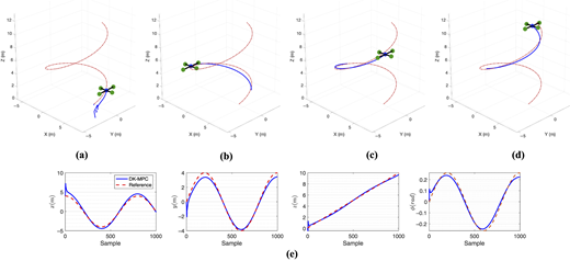
An important observation from the helical trajectory tracking experiment is that the conventional NMPC formulation was unable to find feasible control solutions to follow the desired reference. The strong nonlinearities of the quadrotor dynamics, combined with the complexity of the helical reference path, led to optimization problems that either diverged or failed to converge within the required real-time constraints. As a result, NMPC could not successfully generate control inputs that ensured stable trajectory tracking. In contrast, the proposed DK-MPC framework maintained computational tractability by leveraging a globally linearized Koopman-based model, which enabled efficient optimization at each step as depicted in Figure 10. This distinction underscores the robustness and practicality of the Koopman-based approach for solving constrained trajectory tracking problems in real time, particularly where traditional NMPC struggles to deliver feasible solutions.

While the proposed DK-MPC framework is developed and validated in simulation, its structure is well suited to address real-world challenges that extend beyond the training dataset. In practical deployment scenarios, quadrotors are subject to external disturbances such as wind gusts, parameter drift and sensor noise, all of which may degrade controller performance if not anticipated during the design process. The deep Koopman model provides an advantageous structure for handling such uncertainties, as its learned latent space representation can be enhanced through disturbance-augmented training or domain randomization techniques. Incorporating these variations during training enables the learned Koopman operator to generalize beyond nominal operating conditions and maintain prediction fidelity in the presence of unmodeled effects.

Additionally, the MPC layer inherently supports robustness through constraint tightening, disturbance-aware prediction or tube-based formulations. Such strategies can be integrated without modifying the Koopman representation and allow the controller to remain stable under bounded disturbances. Sensor noise can be mitigated through filtering techniques or by fusing the Koopman model with state estimators, such as extended Kalman filters or Koopman-based observers, further improving reliability in real-world operation. Together, these considerations highlight the adaptability of the DK-MPC approach and its potential to maintain performance when deployed on physical quadrotor platforms exposed to environmental and measurement uncertainties.

In this work, we introduced a DK-MPC framework for quadrotor trajectory tracking and stabilization. By embedding nonlinear dynamics into a lifted linear space via DNNs, DK-MPC enabled computationally efficient MPC formulations that outperformed traditional NMPC in both accuracy and real-time feasibility. Simulation results on trajectory tracking and point stabilization tasks confirmed that DK-MPC significantly reduced tracking errors and achieved average control step times of 15 ms for H = 50, whereas NMPC often failed to provide feasible solutions within real-time constraints. The study highlights three main contributions: (1) the development of a black-box Koopman embedding for quadrotor dynamics trained on flight data; (2) integration of this model with MPC for constrained real-time control and (3) extensive validation against NMPC on challenging trajectories.

The computational efficiency of the DK-MPC approach enables capabilities that are often impractical for conventional NMPC due to real-time computational constraints. In particular, we note that the reduced-order linear structure of the Koopman-based predictor allows faster optimization cycles, which can support higher-frequency control loops, onboard deployment on resource-limited processors and more complex mission objectives requiring long-horizon reasoning. This efficiency also opens the door to advanced functionalities – such as dynamic obstacle avoidance, real-time trajectory re-planning, multi-agent coordination and adaptive control under changing dynamics – that typically exceed the computational budget of full NMPC. By reducing the computational load while preserving nonlinear modeling fidelity, the proposed framework represents a promising step toward enabling more sophisticated autonomous behaviors on real aerial robotic platforms.

Future research will focus on extending DK-MPC towards online or adaptive Koopman learning for robustness under time-varying dynamics and disturbances, deploying the controller on embedded flight hardware to validate on-board real-time performance and scaling the approach to cooperative multi-quadrotor systems. These directions aim to further demonstrate the potential of Koopman-based MPC as a unifying framework for reliable and efficient control in advanced aerial robotics. Meanwhile, future research will extend the Koopman-based predictive control framework to multi-quadrotor systems operating in coordinated formations or platoons [33–35]. In such scenarios, inter-vehicle dynamics introduce additional nonlinear coupling effects that may significantly influence stability, robustness and tracking accuracy.

The supplementary material for this article can be found online.