


This paper aims to analyse gender wage gaps by university majors along the entire wage distribution in Spain before and after the 2008 financial crisis.
The authors perform unconditional quantile regressions to estimate the gender wage gap and use the Oaxaca–Blinder approach to decompose the gender gap.
The observed gender gap among graduates hides significant differences across various fields of study, and both the gap and its unexplained part are highly dependent on the position in the distribution. Engineering and Experimental sciences are the fields with the highest wage differences, and the gap size worsens with the crisis. Health and Humanities, the majors with the highest women presence, show a higher proportion of unexplained part at the bottom tail of the wage distribution, especially after the crisis, suggesting that discrimination against low-paid women has aggravated in these majors.
The paper adds to the existing knowledge by analysing the role that educational decisions play in shaping the wage gap, the variability of the gap along the wage distribution and its response to a change in macroeconomic conditions.
1. Introduction
Gender differences in wages have been extensively analysed in the literature. Although empirical studies suggest that the gender earnings gap has narrowed in developed countries since the 1970s (García-Aracil, 2007), convergence is far from complete. For instance, evidence shows that although women altered their college majors towards those more valuable in the labour market compared to what previous generations have done (Goldin, 2006), women are still concentrated in a small number of industries. Their participation in better-paying jobs is much lower than men’s [1]. In addition, in many countries, women are still assumed to provide unpaid care in the home, which affects their labour market performance (de la Rica and Rebollo-Sanz, 2019). Accordingly, women seem to seek more job flexibility at the cost of high-wage choices (Amuedo-Dorantes and Kimmel, 2005) as they are more compatible with motherhood (Goldin, 2014). Another explanation for this sectoral and occupational segregation, apart from gender differences in preferences and tastes (Zafar, 2013), could be the remaining gender stereotypes in educational choices (Cebrián and Moreno, 2015). The difference in choices in college majors between males and females can have significant economic and social impacts. Differences in returns to majors are much more important than differences in returns to college quality (Arcidiacono, 2004). Previous papers have analysed the marginal effect of fields of study dummies (Gerhart, 1990; Machin and Puhani, 2003; Zając et al., 2023, among others). Lin (2010), Grave and Goerlitz (2012) and Di Paolo and Tansel (2018) instead analysed the gender gap by college major for the cases of Taiwan, Germany and Turkey, respectively. In this article, we follow the latter approach to examine how educational choices have influenced gender labour earnings disparities and its recent evolution in Spain.
Gender differences in the choice of major have been at the centre of intense debate on the reasons behind women’s underrepresentation in majors associated with highly productive economic sectors that could be less affected by economic downturns (Paulsen, 2022). In addition, the behaviour and decisions of women and men vary greatly depending on situations, culture and historical periods (Wood and Eagly, 2012). Despite the similarities in the women’s progress in labour markets experienced in developed countries, an essential variation exists in gender differences in educational decisions and labour pay between countries. This suggests that analysing diverse social and cultural environments is welcome to increase the comprehension of gender wage gaps.
The case of Spain is worth analysing for at least three reasons. Firstly, the recent but rapid incorporation of women into paid work compared to other countries (Távora and Rodríguez-Modroño, 2018). Secondly, female students have been a majority in university classrooms and graduates since the 90s (López Rahona, 2009), but the major choice is still very different between men and women. In 2019, nearly two out of three women graduated in Health, Humanities, Social Sciences and Economics-Law; meanwhile, only one out of three men graduated in these majors. Thirdly, the labour market in Spain traditionally exhibits high levels of labour precariousness due mainly to its deficient regulation and recent flexibilisation (Bentolila et al., 2012; Cárdenas and Villanueva, 2021). In this context, the concentration of women in specific economic sectors and types of contracts (Hidalgo Vega, 2008) has resulted in a social protection system and an employment market that make Spanish women more vulnerable to economic crisis (González Gago and Segales Kirzner, 2014). Murillo-Huertas et al. (2023) multidimensional analysis of precariousness shows similarly worse women’s relative situations in many dimensions of work.
Accordingly, the case of Spain has received increased attention in the literature (Guner et al., 2014). Compared to other European countries, differences in participation, employment and unemployment are persistent (Arrazola and de Hevia, 2006). Furthermore, women have a low presence in male-dominated sectors (Mora and Ruiz-Castillo, 2003; Segovia-Pérez et al., 2020). Men, instead, are found across all occupations, even in professions where women used to be overrepresented. De La Rica et al. (2008) analysed the role of education in wage differences. They found evidence of the glass ceiling hypothesis for the college-educated sample, while the largest differences are at the bottom of the distribution for the non-educated. However, they did not take into account university major choices. Gorjón et al. (2022) analyse the marginal effect of educational decisions on the gender wage gap among young Basque graduates. Results indicate significant differences in the type of contract and salary level, even when women and men have similar academic backgrounds, suggesting that considering educational decisions seems important to understand the Spanish gender wage gap better. This paper adds to the debate by examining the gender wage gap among university majors. As suggested above, major choice can condition the sector and occupations in which graduates can find a job. Therefore, deepening into the disparities that majors can cause could be especially pertinent as economic recessions can affect industries differently (Karamessini, 2014). In this sense, González Gago and Segales Kirzner (2014) showed the different impacts on women’s labour outcomes of the 2008 economic crisis in Spain. In addition, the gender wage gap is not constant across the entire distribution, so the average gender wage gap can obscure interesting differences between low and high-wage workers. Evidence has shown that this is the case for Spain, even after taking into account education attainment (De La Rica et al., 2008) and type of salary (De La Rica et al., 2015) or analysing particular economic sectors (see Casado-Díaz et al., 2022; Segovia-Pérez et al., 2020 for hospitality and Information and Comunication Technology, respectively).
The paper adds to the existing knowledge of the gender wage gap in Spain by (i) focusing on the role that educational decisions play in shaping the gap, (ii) providing new empirical evidence before and after the 2008 economic crisis to show how the gender gap has changed in response to macro-economic conditions and (iii) showing the variability of the gap along the wage distribution. The last contribution is particularly relevant since, to our knowledge, no studies focus explicitly on the heterogeneity across the wage distribution of the relationship between university majors and the gender pay gap.
For that, we use the Survey of Household Finances (SHF) conducted by the Bank of Spain. The period of analysis is 2002–2017. Data availability allows us to identify the major and study the effects (if any) of the last financial and economic crisis. We follow the methodology proposed by Fortin et al. (2011) to analyse the wage gap distribution and decompose these wage differentials across the earnings distribution. This technique offers two improvements. Firstly, as with earnings, it gives robust results when the dependent variable distribution is not symmetric. Secondly, it can provide a disaggregation of earnings distributions that allows testing for differences in wage gap along the earnings distribution.
Results show that observed graduate pay gaps have increased with the crisis, being larger in the upper part of the distribution. The adjusted values, however, are much lower than those observed after the crisis. The individual analysis of the different majors reveals differences in value and trends. Therefore, evidence confirms that educational choices in Spain condition wage differentials between men and women as in other developed countries, even after controlling for individual characteristics and job and sector attributes. The gender wage gap before the crisis seems to be explained mainly by differences in experience and having a part-time job. After the crisis, the different endowments of men and women hardly explain a minimum part, and returns account for most of the observed gap, suggesting a higher degree of discrimination.
The rest of the paper is organised as follows. Sections 2 and 3 present the data and the empirical strategy, respectively. Section 4 shows the results and discussion. Finally, Section 5 concludes.
2. Data and descriptive statistics
To compute wage differences between men and women in Spain, the SHF has been run every three years since 2002 up until 2020, but every two years since 2020. We use waves 2002, 2005, 2008, 2011, 2014 and 2017 [2]. The SHF collects data on wealth, income, debt, consumption and demographic characteristics from a representative sample of Spanish households and their members. The advantage of SHF for our purposes is that it provides detailed information about individuals’ demographic characteristics, occupational classification and labour market experience, the education attained and the field of study. We pool SHF data from different waves as in previous papers with surveys similar to the SHF: Albanesi and Olivetti (2009) for the US Panel Study of Income Dynamics, and Barón and Cobb-Clark (2010) for the Australian Household, Income and Labour Dynamics survey. Although the different waves of the sample have a panel component, we group them for several reasons. Firstly, we concentrate on the gender wage gap analysed in five different majors separately, including quantile regression. This level of disaggregation requires a large size than the one available in each wave of the SHF. Secondly, we are not interested in formally testing for changes over time of individuals but in analysing whether evidence on the gender wage gap changes between the two periods. The pooled sample allows us to speak about changes in population prevalence of attributes, in our case, the wage gap, before and after the crisis. Thirdly, this pooling makes results more robust to events affecting the labour market in specific years, improves the precision of the estimates and can reduce concerns about sample selection. The results can then be interpreted as medium averages of the relevant variables (Albanesi and Olivetti, 2009). In addition, we include robust and cluster errors on each individual to take heteroscedasticity and serial correlation into account. This strategy has been extensively used in previous literature analysing the gender wage gap at different points in time. In addition to Albanesi and Olivetti (2009) and Barón and Cobb-Clark (2010), see, for example, Ghignoni and Pastore (2023), Preston and Birch (2018) or Schollmeier and Scott (2024). We pool data from 2002 to 2008 and from 2011 to 2017 so that the effect of the global 2008 economic crisis can be tackled.
The empirical analysis considers five university majors separately. Namely, Engineering, Health. Humanities, Economics and Law and Experimental. The explanatory variables include individual characteristics, job and firm attributes. The former incorporate years of experience (defined as age-years of education), tenure in the current employment, education (to control if the individual holds a master’s or PhD), number of children in the household and whether they live as a couple. The latter are occupation (ten categories), type of contract (permanent or fixed term), kind of working day (full-time or part-time) and the company’s size (three strata). The analysis is restricted to employed individuals (not devoted to entrepreneurial activities) earning a positive wage. Tables 1 and 2 present descriptive statistics for individual characteristics and job and firm attributes, respectively, for the whole sample, for university graduates and by field of study [3].
Human capital M statistics, men and women
| Whole sample | Graduates | |||||||||||||||||||
|---|---|---|---|---|---|---|---|---|---|---|---|---|---|---|---|---|---|---|---|---|
| Men | Women | Men | Women | |||||||||||||||||
| Before | After | Change | Before | After | Change | Before | After | Change | Before | After | Change | |||||||||
| Panel A | ||||||||||||||||||||
| L hourly wage | 2.06 | 2.11 | 2.43 | 1.81 | 1.89 | 4.42 | 2.49 | 2.52 | 1.20 | 2.24 | 2.25 | 0.45 | ||||||||
| Experience | 23.14 | 24.15 | 4.36 | 20.92 | 23.57 | 12.67 | 19.14 | 21.60 | 12.85 | 16.12 | 20.37 | 26.36 | ||||||||
| Tenure | 10.20 | 11.05 | 8.33 | 8.15 | 10.31 | 26.50 | 13.04 | 12.81 | −1.76 | 10.17 | 12.11 | 19.08 | ||||||||
| Couple | 0.81 | 0.83 | 2.20 | 0.75 | 0.78 | 3.92 | 0.79 | 0.85 | 7.95 | 0.74 | 0.77 | 4.00 | ||||||||
| N. children | 1.43 | 1.24 | −13.00 | 1.33 | 1.17 | −11.74 | 1.36 | 1.22 | −10.26 | 1.25 | 1.16 | −7.81 | ||||||||
| Educ | 7.53 | 4.31 | −42.76 | 8.55 | 4.62 | −45.96 | 36.92 | 17.07 | −53.76 | 27.99 | 12.81 | −54.23 | ||||||||
| Participation | 80.37 | 98.00 | 21.94 | 104.81 | 128.51 | 22.61 | ||||||||||||||
| Wage ratio | 87.86 | 89.57 | 1.95 | 89.96 | 89.29 | −0.75 | ||||||||||||||
| N | 6,541 | 5,555 | −15.07 | 5,257 | 5,444 | 3.56 | 1,995 | 1,894 | −5.06 | 2,091 | 2,434 | 16.40 | ||||||||
| Eng | Health | Human | EconLaw | Exp | ||||||||||||||||
| Men | Women | Men | Women | Men | Women | Men | Women | Men | Women | |||||||||||
| Before | After | Before | After | Before | After | Before | After | Before | After | Before | After | Before | After | Before | After | Before | After | Before | After | |
| Panel B | ||||||||||||||||||||
| L hourly wage | 2.50 | 2.54 | 2.19 | 2.19 | 2.57 | 2.5 | 2.33 | 2.38 | 2.41 | 2.49 | 2.25 | 2.25 | 2.52 | 2.5 | 2.19 | 2.2 | 2.67 | 2.58 | 2.39 | 2.36 |
| Experience | 17.51 | 20.93 | 15.33 | 17.75 | 24.03 | 23.59 | 18.37 | 22.8 | 19.02 | 21.42 | 16.81 | 21.07 | 18.68 | 21.69 | 14.86 | 19.29 | 19.1 | 22.13 | 15.39 | 24.26 |
| Tenure | 11.09 | 11.49 | 8.83 | 9.63 | 17.07 | 15.46 | 13.6 | 16.06 | 12.54 | 13.22 | 10.29 | 12.12 | 12.87 | 12.74 | 8.92 | 10.57 | 14.23 | 12.91 | 9.96 | 14.55 |
| Couple | 0.81 | 0.89 | 0.73 | 0.81 | 0.82 | 0.91 | 0.72 | 0.77 | 0.75 | 0.79 | 0.78 | 0.72 | 0.72 | 0.83 | 0.72 | 0.80 | 0.83 | 0.91 | 0.69 | 0.74 |
| N. children | 0.20 | 0.17 | 0.19 | 0.22 | 0.11 | 0.14 | 0.17 | 0.12 | 0.12 | 0.11 | 0.16 | 0.06 | 0.16 | 0.10 | 0.21 | 0.11 | 0.12 | 0.08 | 0.16 | 0.09 |
| Educ | 36.45 | 12.02 | 21.65 | 9.26 | 44.47 | 12.05 | 41.1 | 15.05 | 30.72 | 20.67 | 27.25 | 13.93 | 36.24 | 18.36 | 26.63 | 10.48 | 57.24 | 29.82 | 48.44 | 31.77 |
| Participation | 23.44 | 34.62 | 179.22 | 270.69 | 187.59 | 214.04 | 113.76 | 144.55 | 84.21 | 129.69 | ||||||||||
| Wage ratio | 87.60 | 86.22 | 90.66 | 95.20 | 93.36 | 90.36 | 86.90 | 88.00 | 89.51 | 91.47 | ||||||||||
| N | 627 | 543 | 147 | 188 | 231 | 174 | 414 | 471 | 282 | 178 | 529 | 381 | 407 | 743 | 463 | 1,074 | 114 | 128 | 96 | 166 |
Mean values. Eng stands for engineering, Human for humanities, EcoLaw for economics and law and Exp for experimental sciences. Participation and wage ratio are the ratio of women to men of number of observations and wages, respectively. Change stands for the percentage change before and after the crisis. Educ includes Master and PhD, participation, wage ratio and change in percentage points
Job descriptive statistics, men and women
| Whole sample | Graduates | |||||||||||||||||||
|---|---|---|---|---|---|---|---|---|---|---|---|---|---|---|---|---|---|---|---|---|
| Men | Women | Men | Women | |||||||||||||||||
| Before | After | Change | Before | After | Change | Before | After | Change | Before | After | Change | |||||||||
| Pannel A | ||||||||||||||||||||
| Occupations (%) | ||||||||||||||||||||
| Manager | 4.39 | 6.02 | 37 | 2.95 | 2.08 | −29 | 12.36 | 18.06 | 46 | 6.04 | 4.54 | −25 | ||||||||
| Scientific, other prof | 8.46 | 11.92 | 41 | 11.71 | 19.74 | 69 | 38.25 | 42.48 | 11 | 35.43 | 50.91 | 44 | ||||||||
| Technician-prof | 12.34 | 11.59 | −6 | 13.85 | 11.79 | −15 | 23.81 | 17.94 | −25 | 25.61 | 15.64 | −39 | ||||||||
| Clerical workers | 8.77 | 7.93 | −10 | 21.23 | 19.24 | −9 | 11.64 | 10.06 | −14 | 23.96 | 19.03 | −21 | ||||||||
| Service, sales workers | 11.77 | 14.1 | 20 | 17.38 | 23.75 | 37 | 5.07 | 6.73 | 33 | 5.24 | 6.33 | 21 | ||||||||
| Skilled agricult | 2.95 | 2.65 | −10 | 1.64 | 0.93 | −43 | 0.46 | 0.21 | −54 | 0.18 | 0.17 | −6 | ||||||||
| Skilled manuf. constr | 21.61 | 17.11 | −21 | 3.88 | 2.62 | −32 | 2.66 | 1.51 | −43 | 0.61 | 0.55 | −10 | ||||||||
| Machine operators | 12.62 | 13.34 | 6 | 1.56 | 1.67 | 7 | 2.17 | 0.75 | −65 | 0.19 | 0.64 | 237 | ||||||||
| Elementary | 15.78 | 13.76 | −13 | 25.53 | 17.73 | −31 | 1.51 | 0.97 | −36 | 2.73 | 2.19 | −20 | ||||||||
| Armed forces | 1.32 | 1.57 | 19 | 0.28 | 0.44 | 57 | 2.08 | 1.28 | −38 | 0 | 0 | |||||||||
| Type of contract (%) | ||||||||||||||||||||
| Permanent | 74.4 | 76.87 | 3 | 65.47 | 72.34 | 10 | 87.68 | 86.26 | −2 | 76.17 | 78.08 | 3 | ||||||||
| Fixed-term | 25.6 | 23.13 | −10 | 34.53 | 27.66 | −20 | 12.32 | 13.74 | 12 | 23.83 | 21.92 | −8 | ||||||||
| Working day (%) | ||||||||||||||||||||
| Full time | 97.35 | 93.42 | −4 | 80.03 | 74.13 | −7 | 95.87 | 92.2 | −4 | 87.59 | 83.96 | −4 | ||||||||
| Part-time | 2.65 | 6.58 | 148 | 19.97 | 25.87 | 30 | 4.13 | 7.8 | 89 | 12.41 | 16.04 | 29 | ||||||||
| Firm size (%) | ||||||||||||||||||||
| < 100 workers | 39.4 | 34.14 | −13 | 42.06 | 32.01 | −24 | 37.16 | 35.99 | −3 | 41.61 | 38.15 | −8 | ||||||||
| 100–499 workers | 36.42 | 35.24 | −3 | 29.72 | 33.19 | 12 | 15.66 | 15.66 | 0 | 11.03 | 12.77 | 16 | ||||||||
| > 500 workers | 24.18 | 30.61 | 27 | 28.22 | 34.8 | 23 | 47.18 | 48.35 | 2 | 47.36 | 49.07 | 4 | ||||||||
| Eng | Health | Human | EcoLaw | Exp | ||||||||||||||||
| Before | After | Before | After | Before | After | Before | After | Before | After | Before | After | Before | After | Before | After | Before | After | Before | After | |
| M | M | W | W | M | M | W | W | M | M | W | W | M | M | W | W | M | M | W | W | |
| Pannel B | ||||||||||||||||||||
| Occupations (%) | ||||||||||||||||||||
| Manager | 10 | 17 | 10 | 5 | 7 | 6 | 2 | 0 | 8 | 8 | 4 | 1 | 18 | 25 | 7 | 7 | 13 | 13 | 17 | 4 |
| Scientific, other prof | 43 | 51 | 32 | 62 | 52 | 65 | 47 | 73 | 43 | 62 | 41 | 68 | 25 | 27 | 23 | 35 | 56 | 47 | 42 | 65 |
| Technician | 32 | 17 | 30 | 13 | 29 | 18 | 38 | 20 | 17 | 16 | 22 | 11 | 24 | 19 | 18 | 15 | 16 | 17 | 23 | 15 |
| Clerical workers | 3 | 3 | 19 | 10 | 4 | 1 | 5 | 1 | 18 | 7 | 22 | 15 | 23 | 19 | 43 | 31 | 3 | 4 | 14 | 10 |
| Service, sales | 1 | 5 | 6 | 6 | 5 | 7 | 5 | 3 | 9 | 4 | 7 | 2 | 4 | 6 | 5 | 8 | 4 | 17 | 2 | 3 |
| Skilled agricult | 1 | 0 | 2 | 0 | 0 | 0 | 0 | 1 | 1 | 0 | 0 | 0 | 0 | 0 | 0 | 0 | 0 | 0 | 0 | 0 |
| Skilled manuf. constr | 4 | 4 | 0 | 4 | 1 | 0 | 1 | 0 | 2 | 1 | 0 | 1 | 1 | 1 | 1 | 0 | 0 | 0 | 0 | 0 |
| Machine operators | 4 | 1 | 0 | 0 | 2 | 1 | 1 | 0 | 0 | 1 | 0 | 1 | 2 | 1 | 0 | 1 | 4 | 0 | 0 | 0 |
| Elementary | 1 | 0 | 2 | 0 | 0 | 1 | 1 | 2 | 2 | 1 | 4 | 1 | 1 | 1 | 3 | 3 | 3 | 2 | 2 | 2 |
| Armed forces | 2 | 1 | 0 | 0 | 0 | 1 | 0 | 0 | 0 | 0 | 0 | 0 | 3 | 1 | 0 | 0 | 0 | 0 | 0 | 0 |
| Type of contract (%) | ||||||||||||||||||||
| Permanent | 86 | 84 | 83 | 80 | 96 | 81 | 75 | 77 | 85 | 85 | 76 | 79 | 86 | 89 | 73 | 77 | 90 | 86 | 94 | 76 |
| Fixed term | 14 | 16 | 17 | 20 | 4 | 19 | 25 | 23 | 15 | 15 | 24 | 21 | 14 | 11 | 27 | 23 | 10 | 14 | 6 | 24 |
| Working day () | ||||||||||||||||||||
| Full time | 97 | 96 | 93 | 87 | 97 | 89 | 89 | 92 | 97 | 89 | 86 | 76 | 94 | 91 | 87 | 84 | 95 | 92 | 94 | 83 |
| Part-time | 3 | 4 | 7 | 13 | 3 | 11 | 11 | 8 | 3 | 11 | 14 | 24 | 6 | 9 | 13 | 16 | 5 | 8 | 6 | 17 |
| Firm size (%) | ||||||||||||||||||||
| < 100 workers | 43 | 44 | 48 | 28 | 32 | 28 | 24 | 28 | 41 | 37 | 43 | 49 | 31 | 34 | 46 | 41 | 32 | 22 | 37 | 29 |
| 100–499 workers | 16 | 14 | 13 | 27 | 12 | 13 | 16 | 8 | 16 | 11 | 10 | 9 | 18 | 18 | 10 | 13 | 15 | 26 | 4 | 17 |
| > 500 workers | 41 | 43 | 39 | 45 | 56 | 59 | 60 | 65 | 43 | 52 | 47 | 42 | 51 | 48 | 44 | 46 | 54 | 52 | 59 | 54 |
Mean values. Eng stands for engineering, Human for humanities, EcoLaw for economics and law, Exp for experimental sciences, Educ includes Master and PhD, Change stands for the change before and after the crisis or each item, in percentage terms, M stands for Men and W for Women
The presence of women in the whole sample is lower than that of men but increased after the crisis. A potential explanation is that during the first years of the economic recession, output and employment contractions were more prominent in industry and construction, where women are consistently underrepresented (Bettio and Verashchagina, 2014). The situation is quite different for graduates. The ratio of employed women to men was 1.05 and 1.28 before and after the crisis, respectively (similar to female university enrolment figures) [4]. However, the number of women and men differs depending on the field of study (see Table 1 panel B). Engineering is the major with a minor percentage of women, whereas women are overrepresented in Health and Humanities. Economics-Law and Experimental are balanced according to EU standards [5]. After the crisis, women’s presence increased in all fields but with different emphases. The wage ratio increased for the whole sample after the economic crisis but was slightly reduced for graduates.
Related to household structure, the number of couples is increasing, but the number of children presents a negative trend. In addition, women have fewer children than men except for Humanities. Despite having fewer children, women have part-time jobs with higher frequency than men in the whole sample, university graduates and all majors, and this percentage has increased in all fields except for health.
Men have more experience and hourly wages than women. Statistics for tenure show that women had less tenure than men before the crisis, but the difference is reduced over the period. For Health and Experimental, women’s tenure increased after the crisis. One possible explanation is that men were more likely to lose their jobs during this economic crisis, as suggested by Guner et al. (2014).
Looking at job type (Table 2), men have managerial jobs more frequently than women before and after the crisis, and this difference increases over time as women, especially graduate women, reduce their presence. The proportion of individuals with permanent jobs is also greater for men. Therefore, the differences between men’s and women’s observed characteristics are generally harmful to female relative wages, except for educational level, in the case of the complete sample. This aligns with previous evidence from Guner et al. (2014).
3. Empirical model and methods
To account for the gender wage gap, we use two complementary analyses. Firstly, we run Mincer regressions to estimate the wage gap that is not accounted for by gender differentials due to individual characteristics and job and firm attributes. The empirical specification is given by:
where LnW is the natural logarithm of gross hourly wages. Female is a gender dummy variable that takes a value of one if the worker is female. X is the set of explanatory variables presented above. The subscript i is omitted. Wave controls have been included in the analysis. The equation is estimated through ordinary least squares (OLS). Still, as wage gaps could be different along the income distribution, and this cannot be captured by traditional OLS estimation, we also use the unconditional quantile regression technique by Fortin et al. (2011). This estimation consists of running a regression of a transformation of the outcome variable (natural logarithm of gross hourly wages), the re-centred influence function, RIF:
where is an indicator function, fy(·) is the density function of the marginal distribution of y, Qτ refers to the τ-quantile of the unconditional distribution of y, c1,τ = 1/fy(Qτ) and c2,τ = Qτ − c1,τ (1 − τ). The RIF will show the influence of an individual on a distributional statistic of interest, in this case the corresponding quantile. This method offers two improvements over OLS that are desirable in this context (Chapman and Lounkaew, 2015). On the one hand, it gives robust results when the dependent variable distribution is not symmetric, as it is the case with earnings. On the other, it provides a disaggregation of earnings distributions.
Secondly, we carry out the Oaxaca (1973),-Blinder (1973) decomposition to explore the relative weights of factors causing wage differentials. The objective is to decompose the wage gap into two parts: one that captures the differences in endowments between women and men (i.e. this part measures the wage penalty derived from their relatively worse characteristics compared with men), and one that measures the extent to which men and women with the similar characteristics receive different returns in exchange for them (this is called the unexplained part and has been frequently considered as measure of discrimination, although it can also capture potential effects of gender differences in unobserved variables). We decompose the gender wage gap for each major average (results in sub-section 4.3) and along the entire distribution. We use the Oaxaca–Blinder decomposition of unconditional quantile regression by Firpo et al. (2018) (results in sub-section 4.4).
The wage differential between males and females can be written in the following way:
where Xfemale and Xmale are the average attributes of the male and female workers, βmale and βfemale are the coefficient estimates from separate regressions for males and females. The first term captures the gender gap that can be accounted for by endowments, which is observed in differences in individual and market labour characteristics between females and males. The second term is the difference in returns of female characteristics. This term is usually interpreted as a measure of discrimination (although it can also capture potential effects of gender differences in unobserved variables). This difference is due to differing rewards for labour market characteristics, usually called the unexplained gender wage gap [6].
Replicate weights and multiple imputations (five imputations) were combined in each estimated model. For each estimation, we specified 200 bootstrap replicates, which ensures that the deviation from the ideal bootstrap standard errors is less than 10% with probability amounting to at least 0.95 (Andrews and Buchinsky, 2000).
4. Results
We estimate the observed and adjusted gender wage gap for each field of study on average terms and for the entire earnings distribution. Since we are pooling different waves, a year control is also included.
4.1 Observed and adjusted wage gaps
The average results are presented in Table 3. The first row of the table shows the observed gender wage gap obtained by regressing log hourly wages on a gender dummy without any additional controls. Panels A and B present the results before and after the crisis.
Gender wage gap
| Observed | Sample | U. grad | Eng | Health | Human | EcoLaw | Exp |
|---|---|---|---|---|---|---|---|
| Panel A: before the crisis | |||||||
| Gender | −0.247*** (0.0155) | −0.249*** (0.0303) | −0.316*** (0.0874) | −0.249*** (0.0757) | −0.156** (0.0731) | −0.330*** (0.0607) | −0.276*** (0.113) |
| Adjusted | |||||||
| Gender | −0.210*** (0.009) | −0.119*** (0.026) | −0.180** (0.083) | −0.112** (0.057) | −0.056 (0.061) | −0.119** (0.051) | −0.192** (0.097) |
| Experience | 0.019*** (0.000) | 0.025*** (0.006) | 0.034*** (0.011) | 0.010 (0.014) | 0.017 (0.011) | 0.034*** (0.013) | −0.009 (0.030) |
| Experience2/100 | –0.035*** (0.001) | −0.035*** (0.012) | −0.045* (0.023) | −0.002 (0.031) | −0.025 (0.024) | −0.044 (0.031) | 0.047 (0.066) |
| Tenure | 0.009*** (0.000) | 0.004 (0.006) | −0.010 (0.013) | 0.008 (0.014) | 0.016 (0.012) | 0.001 (0.015) | 0.015 (0.020) |
| Tenure2/100 | −0.004* (0.002) | 0.003 (0.014) | 0.022 (0.032) | 0.000 (0.034) | −0.016 (0.031) | −0.004 (0.038) | −0.005 (0.052) |
| Master | −0.025*** (0.003) | −0.038 (0.058) | 0.069 (0.165) | −0.053 (0.133) | −0.051 (0.098) | −0.028 (0.110) | 0.048 (0.286) |
| PhD | −0.063*** (0.005) | 0.122*** (0.030) | 0.195*** (0.064) | 0.119 (0.078) | 0.088 (0.073) | 0.098 (0.062) | 0.101 (0.136) |
| Couple | 0.057*** (0.003) | 0.063*** (0.031) | 0.069 (0.060) | 0.028 (0.076) | 0.173*** (0.067) | −0.011 (0.075) | 0.243* (0.136) |
| N. children | −0.007*** (0.001) | 0.011 (0.025) | −0.012 (0.021) | 0.071* (0.040) | −0.001 (0.041) | 0.084 (0.066) | −0.057 (0.051) |
| Fixed term | −0.097*** (0.001) | −0.166*** (0.037) | −0.344*** (0.079) | 0.036 (0.101) | −0.069 (0.090) | −0.139 (0.111) | −0.260 (0.263) |
| Part-time | −0.184*** (0.000) | −0.128** (0.065) | −0.078 (0.127) | −0.192 (0.159) | −0.045 (0.149) | −0.098 (0.133) | 0.003 (0.478) |
| 100–499 | 0.109*** (0.006) | 0.139*** (0.049) | 0.053 (0.071) | 0.063 (0.114) | 0.075 (0.095) | 0.279** (0.135) | −0.062 (0.241) |
| >499 | 0.215*** (0.006) | 0.128*** (0.031) | 0.160** (0.067) | 0.132 (0.096) | 0.104* (0.053) | 0.157** (0.070) | 0.131 (0.157) |
| N | 11,798 | 4,086 | 774 | 645 | 811 | 870 | 210 |
| Panel B: after crisis | |||||||
| Gender | −0.221*** (0.019) | −0.263*** (0.027) | −0.352*** (0.073) | −0.126 (0.078) | −0.244*** (0.087) | −0.302*** (0.048) | −0.214** (0.090) |
| Adjusted | |||||||
| Gender | −0.187*** (0.011) | −0.140*** (0.021) | −0.244*** (0.060) | −0.162** (0.073) | −0.198** (0.080) | −0.076** (0.036) | −0.172*** (0.054) |
| Experience | 0.015*** (0.001) | 0.021*** (0.005) | 0.015 (0.012) | 0.012 (0.014) | 0.019 (0.017) | 0.029*** (0.009) | 0.043*** (0.016) |
| Experience2/100 | −0.023*** (0.002) | −0.024** (0.012) | 0.002 (0.027) | −0.019 (0.028) | −0.034 (0.033) | −0.040** (0.020) | −0.046 (0.031) |
| Tenure | 0.014** (0.000) | 0.027*** (0.005) | 0.036*** (0.012) | 0.041*** (0.012) | 0.032*** (0.013) | 0.022** (0.008) | 0.023** (0.011) |
| Tenure2/100 | −0.014*** (0.002) | −0.052*** (0.016) | −0.090*** (0.035) | −0.076** (0.030) | −0.059* (0.032) | −0.038 (0.024) | −0.054** (0.027) |
| Master | −0.142*** (0.007) | 0.252*** (0.053) | 0.035 (0.116) | 0.179** (0.088) | 0.332*** (0.121) | 0.286*** (0.089) | 0.180 (0.110) |
| PhD | −0.107*** (0.005) | 0.243*** (0.057) | 0.227** (0.101) | 0.259* (0.143) | 0.393*** (0.101) | 0.329** (0.153) | 0.063 (0.057) |
| Couple | 0.070*** (0.003) | 0.014 (0.030) | 0.039 (0.083) | −0.025 (0.086) | 0.038 (0.080) | 0.042 (0.042) | −0.027 (0.081) |
| N. children | −0.028*** (0.001) | 0.023* (0.012) | 0.035 (0.027) | −0.058* (0.034) | −0.040 (0.026) | 0.036* (0.021) | 0.099*** (0.033) |
| Temporary | −0.176*** (0.004) | −0.095** (0.039) | −0.189** (0.084) | 0.084 (0.093) | 0.003 (0.121) | −0.156** (0.062) | −0.125 (0.091) |
| Part-time | −0.141*** (0.000) | −0.216*** (0.046) | −0.222** (0.111) | −0.254** (0.120) | −0.151 (0.108) | −0.276*** (0.072) | −0.276** (0.136) |
| 100–499 | 0.137*** (0.006) | 0.118*** (0.035) | 0.193** (0.094) | −0.026 (0.115) | 0.119 (0.086) | 0.068 (0.055) | 0.268** (0.109) |
| >499 | 0.236*** (0.002) | 0.159*** (0.027) | 0.149** (0.063) | 0.067 (0.085) | 0.115* (0.067) | 0.164*** (0.043) | 0.147** (0.064) |
| N | 10,999 | 4,328 | 731 | 645 | 559 | 1,817 | 294 |
Panel A: OLS estimation with robust and cluster errors. Sample stands for the whole sample, Eng for engineering, Hum for humanities, EcoLaw for economics and law and Exp for experimental sciences. 100–499 and > 499 sizes of the firm (number of workers). The coefficients of occupation, sector and year are not presented for the brevity of exposition. Standard errors are in parentheses. *p < 0.10, **p; < 0.05; ***p < 0.01; Panel B: OLS estimation with robust and cluster errors. Sample stands for the whole sample, Eng stands for engineering, Hum for humanities, EcoLaw for economics and law and Exp for experimental sciences. 100–499 and >499 sizes of the firm (number of workers). The coefficients of occupation and sector are not presented for brevity of exposition. Standard errors are in parentheses. *p < 0.10, **p < 0.05, ***p < 0.01
The observed average gender wage gap estimation for graduates is slightly higher (24.9%) than that of the whole sample (24.7%) (panel A). Pay differences have increased for graduates (+5.62%), while they reduced for the whole sample by 10.5% (Panel B). When job characteristics and human capital features are controlled, the gender wage gap is substantially smaller. This suggests that women’s characteristics and the characteristics of the jobs and sectors where they are most concentrated explain part of the pay differences observed. Interestingly, the graduate-adjusted gender wage gap is now smaller than the sample average as it reduced by 52.2% (46.7%) before (after) the crisis. This would suggest that highly skilled female workers suffer less potential gender discrimination, although the crisis has worsened their situation.
Looking at the different majors, Engineering, Economics-Law (with more than 30% difference) and Experimental are well above the average sample observed gender wage gap. On the other, Humanities is below the sample observed wage gap with the lowest value. Experimental presents the highest adjusted gender wage gap, reduced after the crisis to 17.2%. Engineering shows the second-highest adjusted gender pay gap, increasing after the crisis to 24.4%, becoming the highest gap. Economics and Law present the third-highest gender wage gap. Still, after the crisis, this major has the lowest gap, 7.61%, hence, being the major most affected by human capital and labour market features. On the contrary, Health adjusted gap increases along the period reaching 16.2% and Humanities, where women are overrepresented, shows a remarkable increase in the adjusted wage gap, more than tripling the result before the crisis. This significant heterogeneity in wage rates across college majors is also found in Lin (2010), di Paolo and Tansel (2018) and Zając et al. (2023) for Taiwan, Turkey and Poland, respectively. However, the largest gaps are associated with Medicine, Law and Health and Mathematics.
The results in Table 3 also show some other interesting aspects. Firstly, after the crisis, the penalty associated with part-time work increased for the complete sample and the graduates’ and became significant for all majors except Humanities. This would indicate the crisis's effect on the labour market, in line with the evidence found by Guner et al. (2014). Secondly, the impact of family structure changes with the crisis. The penalty for having children increases for the complete sample after the crisis; however, the Economics and Law and Experimental graduates presented a positive and significant coefficient. Meanwhile, Health shows a children penalty that was not present before, showing disparities among more and less educated individuals and university graduates. Furthermore, it is noteworthy that the sample gap is larger than that found previously (see, e.g. Guner et al. (2014)), which would suggest that the additional observable attributes included (family structure) are generally harmful to female relative wages. In all, this evidence would indicate that some kind of discrimination against women before and after the crisis may be in place and that the crisis impacts different university majors.
4.2 Distribution of gender wage gap
Next, we investigate the observed (see Table 4) and adjusted (see Figure 1) gender wage gaps at different points of the wage distribution. Observed wage gaps for the whole sample are decreasing (increasing) along the wage distribution before and (after) the economic crisis. On the contrary, adjusted gaps present a negative slope, being much steeper after the crisis. Moreover, adjusted gaps are slightly higher than observed in the upper part of the distribution, especially after the crisis, indicating that the potential discrimination against women has aggravated and the glass ceiling effect has sharpened. For graduates, pay gaps have also increased with the crisis, being larger in the upper part of the distribution. However, the adjusted values are lower than those observed after the crisis along the entire distribution. Overall, this evidence suggests that the glass ceiling found in the nineties (De La Rica et al., 2008; Del Río et al., 2011) continues to be an issue in the new century.
Distribution of observed wage gap
| Sample | U grad. | Eng | Health | Human | EcoLaw | Exp | |
|---|---|---|---|---|---|---|---|
| Panel A: before crisis | |||||||
| Mean | −0.247*** (0.0155) | −0.249*** (0.030) | −0.316*** (0.087) | −0.249*** (0.076) | −0.158** (0.073) | −0.330*** (0.061) | −0.276** (0.113) |
| Quantile | |||||||
| Q10 | −0.284*** (0.019) | −0.197*** (0.044) | −0.171 (0.175) | −0.242*** (0.070) | −0.169 (0.108) | −0.200** (0.092) | −0.181 (0.118) |
| Q20 | −0.268*** (0.013) | −0.178*** (0.035) | −0.220 (0.170) | −0.210* (0.121) | −0.115 (0.098) | −0.256*** (0.070) | −0.283** (0.136) |
| Q30 | −0.230*** (0.013) | −0.211*** (0.038) | −0.228 (0.148) | −0.231** (0.112) | −0.221** (0.108) | −0.310*** (0.090) | −0.235 (0.162) |
| Q40 | −0.214*** (0.012) | −0.247*** (0.043) | −0.314** (0.149) | −0.218* (0.116) | −0.225* (0.120) | −0.393*** (0.105) | −0.191 (0.161) |
| Q50 | −0.232*** (0.011) | −0.270*** (0.045) | −0.355** (0.142) | −0.165 (0.112) | −0.217** (0.110) | −0.349*** (0.119) | −0.151 (0.169) |
| Q60 | −0.226*** (0.012) | −0.261*** (0.036) | −0.281** (0.124) | −0.164 (0.119) | −0.190** (0.095) | −0.343*** (0.112) | −0.147 (0.169) |
| Q70 | −0.230*** (0.015) | −0.224*** (0.036) | −0.278** (0.125) | −0.252** (0.123) | −0.158** (0.074) | −0.345*** (0.101) | −0.223 (0.171) |
| Q80 | −0.224*** (0.020) | −0.284*** (0.037) | −0.301*** (0.068) | −0.250* (0.128) | −0.164** (0.073) | −0.321*** (0.091) | −0.336 (0.232) |
| Q90 | −0.198*** (0.022) | −0.263*** (0.042) | −0.385*** (0.079) | −0.290* (0.163) | −0.189** (0.076) | −0.375*** (0.093) | −0.395 (0.270) |
| N | 11,798 | 4,086 | 774 | 645 | 811 | 870 | 210 |
| Panel B: after the crisis | |||||||
| Mean | −0.221*** (0.008) | −0.263*** (0.027) | −0.352*** (0.073) | −0.126 (0.079) | −0.244*** (0.086) | −0.302*** (0.048) | −0.214** (0.090) |
| Quantile | |||||||
| Q10 | −0.161*** (0.024) | −0.164*** (0.046) | −0.137 (0.178) | 0.088 (0.179) | −0.181 (0.116) | −0.202*** (0.077) | −0.220 (0.211) |
| Q20 | −0.185*** (0.014) | −0.222*** (0.040) | −0.229 (0.152) | −0.147 (0.096) | −0.252** (0.101) | −0.274*** (0.058) | −0.408* (0.231) |
| Q30 | −0.172*** (0.013) | −0.279*** (0.037) | −0.267* (0.143) | −0.149 (0.093) | −0.299*** (0.086) | −0.300*** (0.057) | −0.315* (0.164) |
| Q40 | −0.185*** (0.013) | −0.277*** (0.038) | −0.370*** (0.133) | −0.149* (0.086) | −0.245*** (0.085) | −0.376*** (0.068) | −0.114 (0.147) |
| Q50 | −0.197*** (0.012) | −0.268*** (0.039) | −0.430*** (0.103) | −0.127 (0.085) | −0.203* (0.115) | −0.314*** (0.068) | −0.099 (0.103) |
| Q60 | −0.234*** (0.013) | −0.274*** (0.040) | −0.388*** (0.091) | −0.148* (0.083) | −0.167 (0.110) | −0.328*** (0.070) | −0.148 (0.106) |
| Q70 | −0.237*** (0.015) | −0.275*** (0.038) | −0.364*** (0.083) | −0.307*** (0.100) | −0.235** (0.101) | −0.332*** (0.070) | −0.131 (0.102) |
| Q80 | −0.255*** (0.019) | −0.288*** (0.040) | −0.263*** (0.077) | −0.277** (0.129) | −0.219* (0.126) | −0.330*** (0.075) | −0.257 (0.163) |
| Q90 | −0.255*** (0.018) | −0.365*** (0.061) | −0.416*** (0.128) | −0.286* (0.158) | −0.396 (0.256) | −0.387*** (0.106) | −0.439*** (0.160) |
| N | 10,999 | 4,328 | 731 | 645 | 559 | 1,817 | 294 |
Panel A: unconditional quantile regression estimation, Qi stands for the ith quantile. Sample stands for the whole sample, Eng stands for engineering, Hum for humanities, EcoLaw for economics and law and Exp for experimental sciences. Standard errors are in parentheses; *p < 0.10; **p < 0.05, ***p < 0.01; Panel B: unconditional quantile regression estimation, Qi stands for the ith quantile. Sample stands for the whole sample, Eng stands for engineering, Hum for humanities, EcoLaw for economics and law and Exp for experimental sciences. Standard errors are in parentheses; *p < 0.10; **p < 0.05; ***p < 0.01
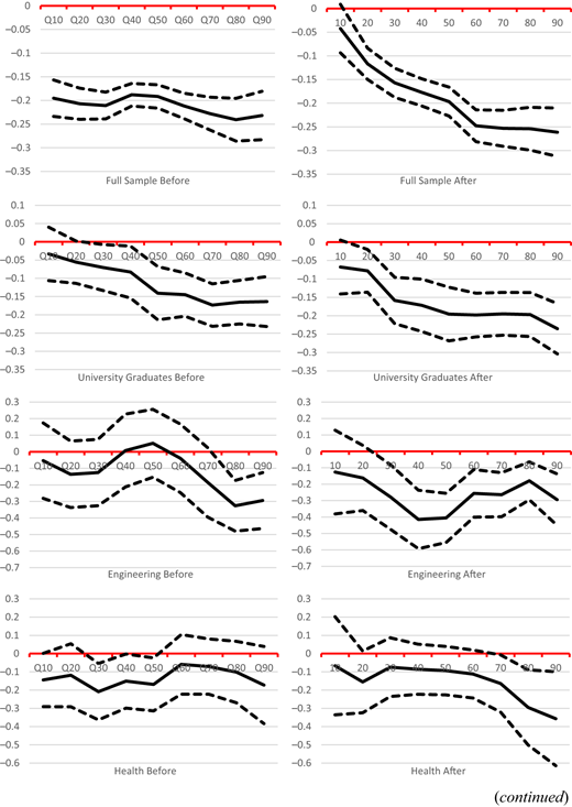
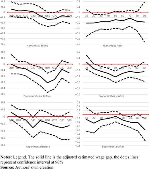
Engineering and Humanities observed gender wage gap has increased along the distribution after the crisis, whereas Health and Economics-Law gender pay differences declined over the period. In the latter case, the gap is larger at the top of the distribution, suggesting some kind of glass ceiling effect.
The analysis of the adjusted gaps by university majors highlights the differences along the wage distribution and diverse evolution. Before the crisis, the Engineering gap showed some kind of inverted U-shape; however, after the crisis, the highest gap was around the median, slightly lower than the observed gap (Table 4). Health-adjusted gender wage gap worsens with the economic crisis in the upper part of the distribution. This evidence indicates a clear glass ceiling effect after the crisis, while no glass ceiling or sticky floor effects existed before (Figure 1). Humanities was the major with the most minor wage discrimination before the crisis, without a significant gender wage gap. However, after the crisis, the gap increased and became statistically significant, particularly at the bottom of the wage distribution, showing some stickiness. Economics-Law presents a kind of U-shape: the gap is larger around the centre of the distribution, but the crisis reduces its value. Experimental presents the glass ceiling effect before and after the crisis.
To summarise, Health and Experimental present glass ceilings, although the gap size evolves differently with the crisis, worsens for the upper part for Health and both tails of the wage distribution in the case of Experimental. Humanities and Economics-Law do not present an increasing gender wage gap, although it worsens for some deciles. Considering majors shows that the glass ceiling effect evidenced for all graduates, in line with De La Rica et al. (2008), is only present for Health and Experimental, especially after the crisis, with the rest of the major gaps much flatter. Interestingly, both majors have participation ratios (number of women over number of men) larger than 100% after the crisis.
4.3 Decomposition of the wage gap
Table 5 presents the results of the Oaxaca decomposition. The first row in the table provides the value of the gender wage gap, and in the rest of the rows, the figures correspond to the different terms of the decomposition (note that a negative value increases the gender wage gap). Differences in the endowments of observed characteristics of men and women do not explain the gender wage gap for the whole sample. Differences in returns are larger than the observed wage gap after the crisis. In the case of graduates, endowments and labour market attributes can explain around 40% of the observed gap before and after the crisis. There are relevant differences among university majors.
Oaxaca decomposition of the wage gap
| Sample | U. grad | Eng | Health | Human | EcoLaw | Exp | |
|---|---|---|---|---|---|---|---|
| Panel A: before crisis | |||||||
| Observed wage gap | −0.247*** | −0.249*** | −0.316*** | −0.249*** | −0.158** | −0.330*** | −0.276** |
| Explained | 0.006 | −0.100*** | −0.073 | −0.142** | −0.082 | −0.223*** | −0.179 |
| Experience | −0.011 | −0.061 | −0.068 | −0.054 | −0.105 | ||
| Tenure | 0.040 | −0.040 | −0.028 | −0.015 | 0.151 | ||
| Education | 0.002 | −0.003 | −0.001 | 0.004 | −0.031 | ||
| N. children | −0.020 | 0.005 | −0.001 | −0.010 | −0.008 | ||
| Temporary | −0.013 | 0.007 | −0.006 | −0.013 | 0.006 | ||
| Part-time | 0.011 | −0.019 | −0.026 | −0.011 | −0.001 | ||
| Manager | −0.046 | 0.008 | −0.001 | 0.007 | 0.001 | ||
| Rest of occupation | −0.041 | −0.032 | 0.015 | −0.117 | −0.042 | ||
| Unexplained | −0.241*** | −0.149*** | −0.243 | −0.107 | −0.076 | −0.107* | −0.097 |
| Panel B: after crisis | |||||||
| Observed wage gap | −0.221*** | −0.263*** | −0.352*** | −0.126 | −0.244*** | −0.302*** | −0.214** |
| Explained | 0.003 | −0.101*** | −0.109 | 0.038 | −0.020 | −0.176*** | −0.009 |
| Experience | 0.043 | −0.011 | −0.014 | −0.046 | 0.112 | ||
| Tenure | −0.045 | 0.030 | −0.029 | −0.036 | 0.026 | ||
| Education | −0.004 | 0.007 | −0.019 | −0.016 | 0.010 | ||
| N. children | −0.003 | 0.009 | −0.004 | 0.006 | −0.010 | ||
| Temporary | −0.006 | 0.005 | 0.013 | −0.026 | −0.017 | ||
| Part-time | −0.017 | 0.005 | −0.016 | −0.015 | −0.021 | ||
| Manager | −0.071 | 0.003 | −0.001 | −0.024 | −0.037 | ||
| Rest of occupation | −0.030 | −0.003 | 0.005 | −0.069 | 0.081 | ||
| Unexplained | −0.224*** | −0.162*** | −0.243*** | −0.164* | −0.224** | −0.125*** | −0.205** |
OLS estimation with robust and cluster errors. Sample stands for the whole sample, Eng stands for engineering, Human for humanities, EcoLaw for economics and law, Exp for experimental sciences. Standard errors are in parentheses. *p < 0.10; **p < 0.05; ***p < 0.01
Before the crisis, the gender wage gap in Engineering is mainly associated with differences in returns (76.8%); Economics and Law, Experimental, Health and Humanities gender wage gaps, on the other hand, are primarily explained by differences in observed characteristics between women and men (67%, 64.8%, 57% and 52%, respectively). The relevance of returns in Engineering wage gap could be connected to gender stereotypes. While there is evidence suggesting a sex difference in mathematics performance (Hyde et al., 2008; De la Rica and Rebollo-Sanz, 2018), the stereotype of women’s inferior performance in mathematics-related tasks is widespread (Guiso et al., 2008). Reuben et al. (2014), in an experimental paper, show that both male and female employers discriminate against women when hiring, often without awareness of their bias.
In addition, the unexplained gap in the different majors could be also related to diverse psychological preferences between men and women. For example, men will be more likely to take up “greedy jobs” (Bertrand, Goldin and Katz, 2010) that demand a greater amount of time but offer extraordinary returns to long working hours. Fields of study differ in the availability of well-paid and likely greedy jobs, which might affect the scope for gender pay gaps and contribute to the observed variation (Zając et al., 2023). Unfortunately, we cannot test these explanations due to data limitations.
The detailed results of the decomposition show, in turn, that the most detrimental factors for female wages are associated with women’s lower endowments of experience, their occupation segregation (more presence in clerical and services occupations and lesser in managerial jobs) and the more part-time contracts signed. Despite these commonalities, the intensity of the hindering effect varies with the major analysed. The evidence also shows some differences related to tenure. In Engineering and experimental, the lower tenure level favours women’s relative wages. The different number of children has a mildly negative impact on women’s wages, except for Health. Similar evidence on the relative importance of work experience and family characteristics is found in Di Paolo and Tansel (2018) for Turkey.
After the crisis, the relevance of differences in returns to explain the wage gap has increased in all majors except for Engineering, which has reduced slightly. However, it explains more than 74%. In the case of Health, Humanities and Experimental, differences in returns explain more than 100%, 91.8% and 95.7% of the raw wage gap, respectively. The differences observed in the unexplained part could be related to distinct characteristics not accounted for in the model that have worsened along the period, such as flexible working hours (less present in Health, for instance).
4.4 Decomposition of the gender gap along the distribution
The proportion of the observed gap not explained by the model (the return component) from the Oaxaca decomposition is depicted for different points of the wage distribution in Figure 2. For the whole sample, the returns component shows a slightly positive trend along the distribution, and this tendency is sharper before the crisis. In the case of graduates, the unexplained content is smaller and more stable. However, a tiny negative trend along the distribution is observed after the crisis. This would suggest that the unfavourable wage treatment suffered by women in relation to men with the same characteristics is relatively uniform along the wage distribution. Looking at the different majors, the return component is more important after the crisis, except for Engineering central deciles. Furthermore, the patterns observed before and after the crisis are quite different for all the majors except for Experimental and Economic-Law, which are similar. Those majors with a more feminine presence, Health and Humanities, present a higher proportion of unexplained parts at the bottom tail of the wage distribution after the crisis, suggesting a relatively worse wage treatment of lower-paid women compared to men with the same characteristics. In the case of Economics and Law, the proportion of the unexplained gap also follows a negative trend and presents much lower values than the former majors.
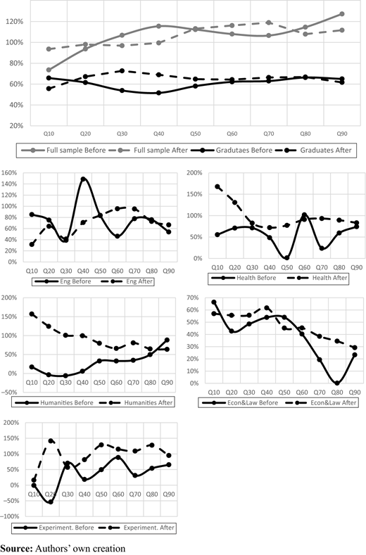
The proportion of the observed wage gap not explained by the model. Before and after the crisis
The proportion of the observed wage gap not explained by the model. Before and after the crisis
5. Conclusion
This paper provides new evidence on the gender wage gap in Spain. The main novelty of the paper is the analysis of the gender wage gap for different college majors and the entire distribution of earnings. Our interest is to show whether educational decisions affect wage differentials and how they evolved after the global economic crisis, which impacted economic sectors differently. We use the SHF prepared by the Bank of Spain to achieve this.
Results confirm the distinct behaviour of the gender gap by education level, as evidenced by De la Rica et al. (2008). Furthermore, university majors present differences in gender wage gaps as in other countries (see, e.g. Lin, 2010; di Paolo and Tansel, 2018; Zając et al., 2023). Engineering, the major with the lowest women participation ratio, has the second largest adjusted gender wage gap. The opposite is true for the Humanities, with the largest women ratio and the smallest gender wage gap before the crisis. Afterwards, both majors’ gender wage gaps worsened, becoming the highest and second highest. The analysis of the wage distribution shows very different behaviours. The largest gap is at the bottom of the distribution in the case of Humanities and around the median in the case of Engineering. No clear sticky floors or glass ceilings emerged. Health and Experimental also present a deterioration of the gender wage gap after the crisis, when the women participation ratio surpassed 100%, especially at the top of the distribution, coherent with the glass ceiling phenomena. Economics and law is the unique major whose gender gap has improved after the crisis.
However, as with all empirical studies, ours has its limitations. We study the impact of educational choices on the gender wage gap using different waves of the SHF survey. We have pooled the data to have enough sample size to analyse university majors separately; however, in some cases, the sample size is still tiny (experimental after the crisis), and results should be interpreted cautiously. The second limitation relates to potential selection bias since educational decisions are not random. Gender gaps in numeracy cognitive skills for adults exist and play a role in explaining gender gaps in labour market performance even when comparing individuals with similar age and education levels (De la Rica and Rebollo-Sanz, 2019). Unfortunately, our data does not have exogenous variation to allow us to control for this potential bias. The next step in our research agenda is to build a larger sample, maybe by reducing major classification and using an alternative empirical strategy to tackle these questions.
Nonetheless, our findings provide interesting and novel evidence. Firstly, the average observed difference in wages between male and female graduates is rather significant, although slightly lower than in the complete sample. In addition, when the wage distribution is considered, the former gap exhibits a much steeper profile than the graduates’ gap, becoming very significant after the crisis in the uppermost part of the distribution, suggesting the presence of a glass-ceiling phenomenon.
Behind the graduates’ gender wage gap, there are important disparities in the magnitude of the differential pay and the diverse pattern along the distribution. Secondly, the decomposition analysis shows that individual endowments and job attributes explain around 40% of the graduates’ gender wage gap. For the complete sample, the observable attributes hardly explain 0.02%, suggesting that women’s endowments in terms of individual characteristics and job attributes should give them access to the same or better wages compared with men, and the crisis has not altered this evidence. This result aligns with previous evidence before the crisis (Casado-Díaz et al., 2022). When looking at the majors, interesting differences emerge. Before the crisis, more than half of the pay differential between men and women in all university majors except for Engineering could be accounted for by observable attributes. Differences in experience, tenure and especially a higher proportion of part-time jobs are the more important attributes of the explained gap, which would be in line with the explanations that suggest that women look for more job flexibility at the cost of high-wage choices (Amuedo-Dorantes and Kimmel, 2005) as they are more compatible with motherhood (Goldin, 2014).
However, after the crisis, the explicative component of observable attributes is much lower, even negligible for Experimental, indicating that this gap is unexplained and accounts for the extent to which men and women with the same characteristics receive different returns in exchange for them. The only exception is Economics and Law, whose observables can partly explain the gap. In particular, 58% of the male–female difference in wages is attributable to the fact that individual and job characteristics of the two groups are different (in particular, women exhibit less tenure and experience and an overrepresentation in less-skilled occupations without more responsibilities). In contrast, the other 43% could be interpreted as resulting from a potential direct discriminatory component.
Overall, the evidence indicates that Spanish graduates are not a homogeneous group and that the relative presence of women in the field does not rule out pay differences or discrimination. Our findings suggest that college majors should be considered when designing policy measures to promote equality and equivalent wages in cooperation with other public policies, as essential differences exist among them.
The authors would like to thank the editor (Olga Cantó) and two anonymous referees for their constructive comments on a previous version of the paper.
Funding: The authors thank support from project PID2019-106642GB-I00 financed by MCIN/AEI/10.13039/501100011033, project PID2020-115018RB-C32, project PID2022-138003NB-I00/MICIU/AEI/10.13039/501100011033/FEDER, UE, and Fundación Cajamurcia.
Notes
See Site to Women's Employmenthttps://ourworldindata.org/female-labor-supply#informal-work-unpaid-care-work on ILO statistical data for 1970-2016 period.
2020 wave is available, but we decided not to include it in the analysis due to the distortional effects of COVID19.
Note that the number of observations of the five majors does not coincide with the total number of graduates due to the existence of respondents who do not identify their major. The answers to the question on the university major have been redefined from the 2014 wave, which could have helped respondents better identify their major and can be behind the increase in the number of graduates in some fields. We consider that not selecting themselves into the right field of study is not correlated to the relevant characteristics of individuals and could be deemed as a random process that affects men and women with differing wage gaps equally
National Statistical Office Homepage to National Statisticalwww.ine.es/jaxiT3/Tabla.htm?t=12722
Stocktaking 10 years of “Women in science” policy by the European Commission 1999–2009.
Estimation of the wage equations is made following the normalization procedure suggested by (Yun, 2005) and as a reference to the pooled model (Oaxaca and Ransom, 1994).

