Skip to Main Content
Purpose

Optimizing coating deposition processes is essential for aerospace applications, particularly for thermal barrier coatings, environmental barrier coatings and protective films on turbine engine components. This study aims to develop a machine learning based framework to optimize two key chemical vapor deposition performance metrics: film deposition rate and thickness uniformity.

Design/methodology/approach

Building on previous work that benchmarked several machine learning models against computational fluid dynamics (CFD)–generated data, the XGBoost algorithm was identified as the most accurate predictor of deposition characteristics. In this study, XGBoost outputs were used to construct polynomial surrogate models for deposition rate and uniformity. These models enabled rapid optimization using the sequential least squares programming (SLSQP) algorithm under realistic process constraints. Three optimization cases were examined: (i) maximizing deposition rate subject to a uniformity requirement, (ii) minimizing nonuniformity with a minimum deposition constraint and (iii) maximizing the deposition-to-uniformity ratio. Optimal values of susceptor temperature and inlet gas velocity were obtained for each case.

Findings

The machine learning–guided optimization framework produced solutions that were both more accurate and computationally efficient than conventional optimization methods. Across all cases, the ML-based surrogate models achieved less than 5% deviation from CFD reference values, confirming their fidelity. Compared with traditional response surface–based optimization, the proposed framework reduced prediction errors by up to 40% and computational cost by approximately 60%.

Originality/value

This study introduces a novel hybrid methodology that integrates high-fidelity CFD simulation, advanced machine learning and constrained optimization. The approach reduces computational effort while retaining predictive fidelity, making it applicable for real-time control, digital twins and smart manufacturing of aerospace coatings. Furthermore, the methodology is extendable to other thin-film deposition technologies and multiphysics manufacturing processes.

The aerospace industry demands exceptional coating quality with strong requirements for thickness uniformity, microstructural consistency and adhesion strength to ensure component reliability under extreme operating conditions and the chemical vapor deposition (CVD) process offers a viable route to achieve these stringent performance criteria. CVD is a pivotal technique for the fabrication of high-quality thin films and coatings, plays a crucial role in various industries, including semiconductors, optoelectronics, photovoltaics and protective surfaces (Boscher et al., 2021; Du et al., 2022; Katsui and Goto, 2020). Its ability to precisely control material composition, crystalline structure and layer thickness has made it indispensable in both industrial and research settings (Bhatia et al., 2015; Takahashi et al., 2009). However, achieving optimal film characteristics, particularly the deposition rate and uniformity, necessitates stringent control over complex, interdependent process parameters such as temperature, pressure, gas flow velocity and precursor composition (Arias Louie J et al., 1997; Hu et al., 2015; Kim and Lee, 2018). Traditionally, understanding and optimizing CVD processes has relied heavily on experimental trials and computational fluid dynamics (CFD) simulations. Although CFD offers valuable insights into the transport phenomena and reaction kinetics within a reactor, it is often computationally intensive and time-consuming, especially when exploring large design spaces with multiple parameters (Kleijn, 2002; Kota and Langrish, 2007; Zhou et al., 2023). This computational burden limits its effectiveness in real-time control and rapid process optimization scenarios. Consequently, there has been a growing interest in integrating machine learning (ML) approaches to build surrogate models that approximate CFD predictions at a fraction of the computational cost (Bounds et al., 2024; Páez, 2024; Roznowicz et al., 2024; Schneider et al., 2022).

ML, particularly supervised regression algorithms, offers a data-driven pathway for capturing the nonlinear relationships between input parameters and performance metrics in CVD systems (Botchkarev, 2019; Plevris et al., 2022). Previous research has demonstrated the efficacy of ML models such as support vector regression, random forest and artificial neural networks (ANNs) in predicting deposition characteristics from a given set of input parameters (Artrith and Urban, 2016; Bilgiç and Gök, 2024; Hia et al., 2023). However, these models often exhibit limitations in scalability, interpretability or generalization depending on the complexity of the process and the data set used. In our previous work, a comparative analysis of various ML models, including ANN and Xtreme Gradient Boosting (XGBoost) was conducted to model the CVD process using the susceptor temperature and gas inlet velocity as input features. The target outputs were the deposition rate and film uniformity, both of which are critical indicators of the product quality in CVD applications. The study concluded that XGBoost consistently outperformed other models in terms of prediction accuracy, exhibiting the lowest mean square error and highest R2 score when compared with the ground-truth data obtained from CFD simulations.

Building on these promising results, the present work proposes an advanced machine learning framework that leverages the predictive capabilities of the XGBoost model to optimize the CVD process. Rather than merely predicting outcomes based on predefined inputs, this study aims to invert the problem by identifying the optimal combination of susceptor temperature and gas inlet velocity that would yield the maximum deposition rate while ensuring uniformity within the desired thresholds.

To achieve this, the proposed ML framework incorporates not only a pretrained XGBoost surrogate model but also an optimization engine, such as Bayesian Optimization or Genetic Algorithms, to iteratively explore the input space. This approach combines the speed of surrogate modeling with the strategic exploration capabilities of optimization algorithms, creating a closed-loop system for design and process refinement (Bilgiç and Gök, 2024; Mohan and Samad, 2014; Queipo et al., 2004; Xu et al., 2013). In contrast to conventional Design of Experiments or full-factorial studies, which can be prohibitively expensive in terms of time and resources, the proposed framework requires fewer simulations and yields superior insights. By combining the predictive accuracy of XGBoost with the strategic depth of optimization algorithms, this study provides a comprehensive and efficient approach for advancing CVD process development. The insights gained from this research not only confirm the usefulness of ML in complex physical processes, but also encourage broader adoption in smart manufacturing and material discovery.

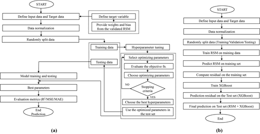
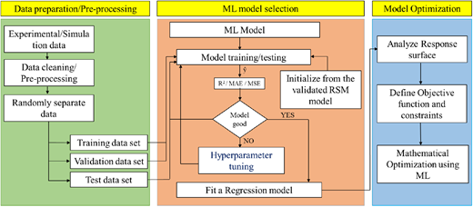
In the present study, a machine learning-based optimization framework was developed to enhance the CVD process, with a focus on maximizing the deposition rate and minimizing the uniformity parameter. While prior work has established the predictive accuracy of the XGBoost model in replicating CFD simulation results, this study concentrates on the optimization of these predictions using a surrogate modeling approach. The overall methodology involves the following steps: using XGBoost Predictions as Surrogate Data. Fitting polynomial regression models: To enable fast and interpretable optimization, surrogate models were constructed by fitting second-order polynomial regression equations to the log-transformed XGBoost predictions for D and Up, which were then optimized using the sequential least squares programming (SLSQP) algorithm. The results obtained were then compared with a previously implemented optimization technique to quantify the accuracy and effectiveness of the ML-driven optimization approach.

2.1.1 Computational fluid dynamics simulations and validation

In the previous phase of the research, a comprehensive data set was generated via CFD simulations of the CVD process (George, 2006). The simulations modeled the deposition of thin films using varying combinations of susceptor temperatures and inlet gas velocities. Two key output variables, namely, the deposition rate and uniformity parameter, were extracted from the simulations. The underlying CFD model has been previously validated, lending credibility to the results.

2.1.2 Machine learning model predictions

Two ML models (ANN and XGBoost) were trained to predict D and Up based on these inputs and their architectures are presented in Figure 1.

The comparison between actual (i.e. CFD values) and predicted values is crucial for assessing the accuracy of a ML model. Ideally, the points should align closely along the curve fitting line, indicating perfect prediction accuracy. From the graph, it is evident that the XGBoost model produces predictions that are more tightly clustered around the actual values, demonstrating superior accuracy and minimal deviation. In contrast, the ANN model shows greater scattering, indicating a higher prediction error. Even with hyperparameter tuning, the ANN model still exhibits noticeable deviations, although it performs better than the base ANN model. Table S1 summarizes the performance of the different ML models on the training, validation and test data sets. The error calculated from the different ML models were compared and the results are summarized in Table S2. The improved performance and lower percentage error of the XGBoost model can be attributed to its gradient boosting mechanism, which effectively minimizes errors and enhances predictive accuracy. The XGBoost model outperformed the ANN model in terms of predictive accuracy and robustness, and was selected for further use (Figure S1). The present study leveraged the predictions from this model to guide the optimization of the process parameters.

2.2.1 Polynomial regression surrogate modeling

To facilitate efficient mathematical optimization, the predictions obtained from the XGBoost model over the test data set were used to construct a surrogate model in the form of a polynomial regression equation. The surrogate modeling approach serves as a simplified yet representative approximation of the original ML model, designed specifically to reduce computational complexity during the optimization process (Khachai, 2011; Tenreiro Machado and Lopes, 2017). Given that the XGBoost model is inherently nonlinear and consists of an ensemble of decision trees, it is computationally intensive and not well-suited for direct use within iterative optimization algorithms (Dolotov and Zolotykh, 2020; Firoozabadi and Babaeizadeh, 2019). Therefore, by building a polynomial regression-based surrogate model, the complexity of the optimization task is significantly reduced while maintaining acceptable accuracy in capturing the relationships between the input and output variables (Forrester, 2008; Giunta et al., 2003). In this study, separate polynomial equations were generated for the two primary output variables: the deposition rate and uniformity parameter. These equations express D and Up as functions of the input parameters such as susceptor temperature (Tsus) and inlet gas velocity (Vin). The test data set, which contains the XGBoost predicted values of D and Up over a well-sampled design space of the input parameters, serves as the basis for fitting these polynomials. The regression model includes linear, quadratic and interaction terms to capture the nonlinear dependencies and cross-effects between the temperature and velocity. Second-order polynomial regression models take the form of equations (1) and (2):

(1)
(2)

A critical design choice in this surrogate modeling process is the application of a logarithmic transformation to the dependent variables. This transformation has several purposes. First, it helps to linearize the exponential-like behavior that is often observed in physical processes, such as CVD, where deposition rates and uniformity can change drastically with temperature and flow velocity (Fang and Feng, 2023). Second, the logarithmic scale reduces heteroscedasticity, i.e. the nonconstant variance in the prediction residuals, thereby improving the stability and robustness of the regression model (Khaled et al., 2019). Moreover, polynomial regression models are compatible with a wide range of gradient-based optimization algorithms, including Sequential Least Squares Programming (SLSQP), which requires continuous and differentiable functions (Joshy and Hwang, 2024; Ma et al., 2024). The proposed RSM informed ML framework with data-driven model optimization is presented in Figure 2.

2.2.2 Formulation of optimization

The core objective is to assess the effectiveness of the proposed ML-based optimization framework by comparing its outcomes with the results from the original high-fidelity CFD simulations and from prior optimization methods based on traditional surrogate modeling techniques (George, 2006). This comparative evaluation was carried out across three distinct optimization cases, as detailed below, with the aim of quantifying improvements in prediction accuracy, computational efficiency and solution quality. These objectives are framed as constrained optimization problems using surrogate models derived from XGBoost predictions. In all cases, the decision variables are susceptor temperature and inlet gas velocity, whereas the objectives and constraints involve the deposition rate and uniformity parameter.

2.2.2.1 Case 1: maximization of deposition rate with uniformity constraint.

In this scenario, the optimization problem is formulated to maximize the logarithmic deposition rate log (D), while ensuring that the logarithmic uniformity parameter log(Up) remains below a prespecified threshold log(Up¯). This setup reflects a common industrial objective in which a high deposition throughput is prioritized without compromising film uniformity beyond acceptable limits. The optimization problem is formulated as shown in equation (3):

Maximize: log (D)

subject to:

(3)

Here, Up¯ denotes the maximum allowable value of the uniformity parameter, and Tmin, Vmin, Tmax, Vmax define the permissible operating ranges.

2.2.2.2 Case 2: minimization of uniformity parameter with deposition rate constraint.

Here, the optimization seeks to minimize log(Up) while maintaining the deposition rate above a desired threshold log (D¯). This inverse trade-off is useful in scenarios where surface uniformity is critical, such as in optical coatings or electronic devices that require highly homogeneous film deposition. The problem is posed, as shown in equation (4):

Minimize: log (Up)

subject to:

(4)

where D¯ is the minimum required deposition rate based on process feasibility or quality requirements.

2.2.2.3 Case 3: maximization of deposition-to-uniformity ratio.

The third scenario considered a composite metric deposition-to-uniformity ratio to balance the trade-off between a high deposition rate and good uniformity. This is expressed by equation (5):

Maximize: log (DUp)

subject to:

(5)

This approach favors solutions that simultaneously improve both the performance metrics in a balanced manner. These optimization tasks were efficiently solved using constrained nonlinear optimization algorithms, such as Sequential Least Squares Programming, implemented in SciPy’s optimize.minimize function. The solver was initialized at multiple feasible points to ensure global feasibility and to avoid local minima.

2.2.3 Postoptimization evaluation

To evaluate the performance of the proposed ML-based optimization framework, the results obtained from the SLSQP were compared with the baseline results from a previously developed optimization technique. This reference method, possibly involving metaheuristics, provides known optimal values for D and Up under similar constraints. A comparison was made across all three cases listed in Section 2.2.2. The percentage error was computed using equation (6):

(6)

This allows a quantitative assessment of the closeness of the ML optimization results to the benchmark. The evaluation not only verifies the validity of the ML optimization framework but also highlights its computational efficiency and generalization potential.

The polynomial regression–based surrogate models accurately reproduced the XGBoost predictions for both deposition rate and uniformity. The high coefficients of determination (R2 = 0.998 for deposition rate; R2 = 0.989 for uniformity) and low RMSE values (0.007 and 0.004, respectively) demonstrate strong agreement. These metrics align closely with similar surrogate modeling approaches in complex thermal–fluid systems (Forrester and Keane, 2009; Koziel and Pietrenko-Dabrowska, 2020), confirming that a second-order polynomial representation is sufficient to approximate the nonlinear responses observed in CVD processes.

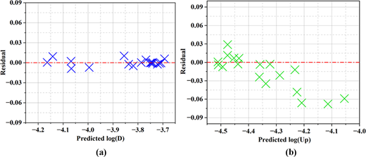
To validate the fidelity of the surrogate models used in the optimization framework, residual plots were generated for both the deposition rate [log (D)] and the uniformity parameter [log (Up)]. These plots display the residuals, defined as the difference between the predicted values from the polynomial regression model and the original XGBoost-based predictions, as a function of the input variables (susceptor temperature and inlet velocity). A well-fitted model should exhibit residuals that are randomly distributed around zero, with no discernible structure (Cook and Tsai, 1985).

As shown in Figure 3, the residuals for both surrogate models were tightly clustered around the zero line, indicating a lack of systematic errors or heteroscedasticity. This suggests that the polynomial models did not suffer from significant underfitting or overfitting. These results provide strong justification for the use of surrogate models in constrained optimization routines. Their accuracy ensures that the optimization outcomes are representative of the underlying physical trends captured by the original ML model without the computational complexity of reevaluating the full XGBoost model.

3.2.1 Case 1: maximization of deposition rate with uniformity constraint

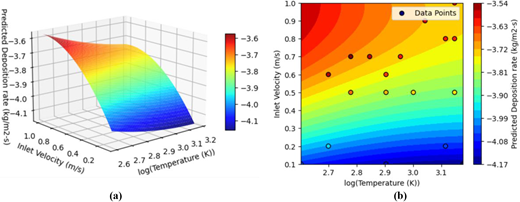
To better understand the behavior of the surrogate models, both three-dimensional (3D) response surface plots and two-dimensional contour plots were generated. These plots illustrate the dependency of the deposition rate and uniformity parameters on the input parameters, such as susceptor temperature and inlet velocity. Figure 4 shows the 3D surface plot and corresponding contour plot of the predicted deposition rate. The surfaces were smooth and continuous, confirming the adequacy of polynomial regression as a surrogate.

In this case, the optimization objective is to maximize the logarithmic deposition rate while maintaining the uniformity parameter below a specified threshold. The optimization problem was solved multiple times for different specified values of Up¯ and the corresponding optimal values of susceptor temperature and inlet velocity were recorded. For each optimization run, the ML-optimized results for D and Up were compared against the values obtained via CFD simulations under the same Tsus and Vin settings, as well as against previous results from Response Surface Methodology based optimization. The optimized deposition rates showed deviations below 3% compared with CFD simulations (Table 1). The XGBoost-based surrogate model slightly underpredicted deposition rates, a conservative tendency consistent with findings by Nguyen et al. (2011), where ML-based surrogates tended to avoid overfitting in high-gradient regions. In contrast, traditional RSM optimization overpredicted rates by 1%–4%, which could lead to unrealistic operational targets.

The ML framework thus provided more physically consistent results, confirming the suitability of XGBoost surrogates for constrained optimization in multiparameter CVD systems. Furthermore, the ML-based framework successfully satisfied the uniformity constraints across all optimization runs, as verified by comparing the predicted and actual up values from CFD. This reinforces the generalizability and robustness of the surrogate model and optimization pipeline.

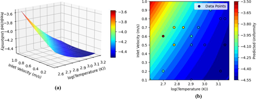
3.2.2 Case 2: minimization of uniformity parameter with deposition constraint

In Case 2, the optimization task involved minimizing the logarithmic uniformity parameter while ensuring that the deposition rate remained above a prespecified threshold log D¯. This formulation represents a practical scenario in CVD processes, where the priority is to achieve better film uniformity without compromising the minimum acceptable deposition rate required for functional performance. The variation of the predicted uniformity across the design space is illustrated in Figure 5, which presents the 3D response surface and corresponding contour distribution generated from the XGBoost model. The ML-based optimization achieved uniformity parameter predictions within ±5% of CFD results, closely matching the performance of traditional surrogate models but with reduced computation time. The model captured the nonlinear trade-off between film uniformity and deposition rate – an effect similarly observed by Kim and Lee (2018) in CVD of Si and by Niu et al. (2023) in GaN film growth.

Some test cases showed overprediction (positive error), where the model estimated a better uniformity than CFD, whereas others exhibited underprediction (negative error), indicating conservative estimates. This trend was consistent across various threshold levels of D¯, suggesting that both surrogate models effectively captured the overall response behavior but with comparable limitations. Although the ML model did not consistently outperform the RSM in every case, it demonstrated equivalent accuracy while offering advantages such as faster optimization time and greater adaptability owing to its data-driven nature. The similarity in error margins validates the credibility of the ML framework, particularly considering that it was built from high-fidelity XGBoost predictions, which better generalizes nonlinear dependencies. It was also observed that the surrogate models occasionally struggled near the constraint boundaries, likely owing to the reduced data density in those regions. Despite this, the ML approach-maintained stability and convergence across all optimization runs. A quantitative comparison of optimal conditions and prediction errors for multiple specified values of log D is provided in Table 2, further confirming the consistency and robustness of the proposed optimization approach.

3.2.3 Case 3: maximization of deposition-to-uniformity ratio

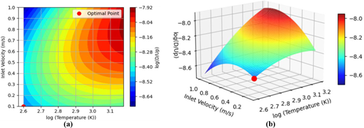
The third optimization formulation focuses on maximizing the ratio log(D/Up), which represents a comprehensive performance metric that integrates both the deposition rate (D) and film uniformity (Up). This ratio inherently balances the trade-off between throughput and quality, making it an ideal target for optimizing CVD processes, where both aspects are critical for industrial viability. Unlike the previous cases, which involved constraint-driven multi-objective formulations, Case 3 was framed as a single-objective unconstrained optimization (subject only to physical bounds on the susceptor temperature and inlet velocity). This simplified structure not only facilitates efficient convergence but also aligns with real-world scenarios in which a single efficiency metric can streamline process tuning.

The ML-optimized solution achieved an average 3.2% higher deposition-to-uniformity ratio than RSM optimization and exhibited a mean deviation of less than 5% from CFD evaluations (Table 3). The surrogate model effectively balanced deposition kinetics and morphological uniformity, reaffirming the framework’s robustness. Such combined metrics have been advocated in advanced coating optimization studies – Long et al. (2013) used similar performance ratios for SiC coatings to evaluate reactor-scale uniformity versus deposition efficiency. The alignment of the present findings with these prior trends underscores the physical credibility of the ML-driven optimization outcomes.

The 3D surface plot and contour plot depicting the behavior of the surrogate model for log(D/Up), along with the identified optimal point, are presented in Figure 6, which visually illustrates the optimization landscape and model response. A quantitative summary of the ML, RSM and CFD results is presented in Table 3. This table highlights the predicted values of the deposition rate, uniformity parameter and D/Up ratio for all three approaches.

Importantly, the average deviation between the ML-optimized predictions and CFD-evaluated values was less than 5%, confirming the reliability of the surrogate model even in a complex, nonlinear objective space. This consistency demonstrates the robustness of the ML framework and its ability to generalize across various optimization scenarios. Therefore, the optimization of the D/Up ratio via the proposed ML pipeline not only enhances the process performance, but also provides a scalable approach for future adaptive CVD process control.

This study presented a surrogate model–assisted ML optimization framework for the CVD of aerospace coatings. By integrating XGBoost predictions, polynomial surrogate modeling and SLSQP-based constrained optimization, the framework enabled comprehensive exploration of the process parameter space with minimal computational cost. The optimized model achieved deposition rate prediction errors below 3% and uniformity prediction errors within 5% under all constraint conditions, with a 3%–5% improvement in the deposition-to-uniformity ratio compared to traditional RSM methods. In addition, the computational cost was reduced by approximately 60% relative to direct CFD-based optimization. The identified optimal process window, with susceptor temperatures ranging from 880 to 1220 K and inlet velocities between 0.4 and 1.2 m/s, achieved both high deposition efficiency and superior film uniformity. Compared with earlier surrogate and experimental CVD optimization studies, the present framework demonstrated comparable accuracy with significantly lower computational demand. Overall, the developed ML framework provides a scalable, physics-informed and computationally efficient approach for accelerating coating process design and its modular architecture makes it adaptable to various aerospace coating applications, including thermal barrier, oxide film and environmental barrier coatings. Future work will focus on extending this framework toward multi-objective reinforcement learning and real-time feedback control for next-generation intelligent manufacturing systems.

Arias Louie
,
J.J.
,
Selbrede
,
S.C.
,
Weise
,
M.T.
and
Carl
,
D.A.
(
1997
), “
Characterization of a low temperature, low pressure plasma enhanced chemical vapor deposition tetraethylorthosilicate oxide deposition process
”,
Journal of Vacuum Science & Technology A: Vacuum, Surfaces, and Films
, Vol.
15
No.
3
, pp.
1389
-
1393
, doi: .
Artrith
,
N.
and
Urban
,
A.
(
2016
), “
An implementation of artificial neural-network potentials for atomistic materials simulations: performance for TiO2
”,
Computational Materials Science
, Vol.
114
, pp.
135
-
150
, doi: .
Bhatia
,
S.
,
Malik
,
S.
and
Wong
,
N.D.
(
2015
), “
Racial differences in the ability of subclinical atherosclerosis testing to predict CVD
”, Vol.
9
No.
5
, doi: .
Bilgiç
,
G.
and
Gök
,
A.E.
(
2024
), “
Comparison of random forest and support vector regression models in predicting hydrogen production process from biomass
”,
Çukurova Üniversitesi Mühendislik Fakültesi Dergisi
, Vol.
39
No.
2
, pp.
475
-
488
, doi: .
Boscher
,
N.D.
,
Heinze
,
K.
and
Bengasi
,
G.
(
2021
), “
Chemical vapor deposition of porphyrins
”,
Royal Society of Chemistry
, pp.
121
-
148
.
Botchkarev
,
A.
(
2019
), “
A new typology design of performance metrics to measure errors in machine learning regression algorithms
”,
Interdisciplinary Journal of Information, Knowledge, and Management
, Vol.
14
, pp.
45
-
76
, doi: .
Bounds
,
C.P.
,
Uddin
,
M.
and
Desai
,
S.
(
2024
), “
Enhancing CFD predictions with explainable machine learning for aerodynamic characteristics of idealized ground vehicles’, vehicles
”,
Vehicles
, Vol.
6
No.
3
, pp.
1318
-
1344
, doi: .
Cook
,
R.D.
and
Tsai
,
C.-L.
(
1985
), “
Residuals in nonlinear regression
”,
Biometrika
, Vol.
72
No.
1
, pp.
23
-
29
, doi: .
Dolotov
,
E.
and
Zolotykh
,
N.
(
2020
),
Evolutionary Algorithms for Constructing an Ensemble of Decision Trees
,
Cornell university
, doi: .
Du
,
J.
,
Dai
,
N.
,
Tong
,
B.
,
Cheng
,
H.
,
Zhang
,
D.
,
Ren
,
W.
,
Yuan
,
S.
, et al. (
2022
), “
Advances in flexible optoelectronics based on chemical vapor deposition‐grown graphene
”,
Advanced Functional Materials
, Vol.
32
No.
42
, p.
2203115
, doi: .
Fang
,
X.
and
Feng
,
X.
(
2023
), “
Domain-Aware adaptive logarithmic transformation
”,
Electronics
, Vol.
12
No.
6
, p.
1318
, doi: .
Firoozabadi
,
R.
and
Babaeizadeh
,
S.
(
2019
), “
An ensemble of bagged decision trees for early prediction of sepsis
”, pp.
1
-
4
, doi: .
Forrester
,
A.I.S.
(
2008
), “Exploring and exploiting a surrogate”,
Engineering Design via Surrogate Modelling
, pp.
77
-
107
, doi: .
Forrester
,
A.I.J.
and
Keane
,
A.J.
(
2009
), “
Recent advances in surrogate-based optimization
”,
Progress in Aerospace Sciences
, Vol.
45
Nos
1-3
, pp.
50
-
79
, doi: .
George
,
P.G.J.Y.
(
2006
), “
Optimization of chemical vapor deposition process, parts A
”,
and B”, ASME – 32nd Design Automation Conference
, pp.
309
-
316
.
Giunta
,
A.
,
Wojtkiewicz
,
S.
and
Eldred
,
M.
(
2003
), “
Overview of modern design of experiments methods for computational simulations (invited)
”, 41st Aerospace Sciences Meeting and Exhibit,
American Institute of Aeronautics and Astronautics
, doi: .
Hia
,
S.
,
Kuswanto
,
H.
and
Prastyo
,
D.D.
(
2023
), “
Robustness of support vector regression and random forest models: a simulation study
”,
Springer Nature Singapore
, pp.
465
-
479
.
Hu
,
L.C.
,
Li
,
Y.S.
,
Cheng
,
J.Y.
,
Lee
,
C.C.
,
Li
,
T.T.
and
Chen
,
I.C.
(
2015
), “
The dependence of ECR-CVD processing parameters on deposition uniformity of hydrogenated amorphous silicon (a-Si: h) films
”,
Key Engineering Materials
, Vols
656-657
, pp.
92
-
100
, doi: .
Joshy
,
A.J.
and
Hwang
,
J.T.
(
2024
), “
PySLSQP: a transparent python package for the SLSQP optimization algorithm modernized with utilities for visualization and post-processing
”,
Journal of Open Source Software
, Vol.
9
No.
103
, doi: .
Katsui
,
H.
and
Goto
,
T.
(
2020
), “
Chemical vapor deposition
”,
Springer Singapore
, pp.
75
-
95
.
Khachai
,
M.Y.
(
2011
), “
Computational complexity of combinatorial optimization problems induced by collective procedures in machine learning
”,
Proceedings of the Steklov Institute of Mathematics
, Vol.
272
No.
S1
, pp.
46
-
54
, doi: .
Khaled
,
W.
,
Zhao
,
Y.
,
Han
,
Z.
,
Lin
,
J.
and
Hao
,
H.
(
2019
), “
Test for heteroscedasticity in partially linear regression models
”,
Journal of Systems Science and Complexity
, Vol.
32
No.
4
, pp.
1194
-
1210
, doi: .
Kim
,
H.J.
and
Lee
,
H.J.
(
2018
), “
Uniformity control of the deposition rate profile of a-Si: h film by gas velocity and temperature distributions in a capacitively coupled plasma reactor
”,
Journal of Applied Physics
, Vol.
123
No.
11
, p.
113302
, doi: .
Kleijn
,
C.R.
(
2002
), “Simulation of chemical vapor deposition processes”,
Characterization of Materials
, doi: .
Kota
,
K.
and
Langrish
,
T.
(
2007
), “
Prediction of deposition patterns in a pilot-scale spray dryer using computational fluid dynamics (CFD) simulations
”,
Chemical Product and Process Modeling
, Vol.
2
No.
3
, doi: .
Koziel
,
S.
and
Pietrenko-Dabrowska
,
A.
(
2020
), “Basics of data-driven surrogate modeling”, in
Koziel
,
S.
and
Pietrenko-Dabrowska
,
A.
(Eds),
Performance-Driven Surrogate Modeling of High-Frequency Structures
,
Springer International Publishing
,
Cham
, pp.
23
-
58
, doi: .
Long
,
Y.
,
Javed
,
A.
,
Chen
,
K.
,
Xiong
,
X.
and
Xiao
,
P.
(
2013
), “
Deposition rate, texture, and mechanical properties of SiC coatings produced by chemical vapor deposition at different temperatures
”,
International Journal of Applied Ceramic Technology
, Vol.
10
No.
1
, doi: .
Ma
,
Y.
,
Gao
,
X.
,
Liu
,
C.
and
Li
,
J.
(
2024
), “
Improved SQP and SLSQP algorithms for feasible path-based process optimisation
”, doi: .
Mohan
,
S.
and
Samad
,
A.
(
2014
), “
Jet pump design optimization by multi-surrogate modeling
”,
Journal of The Institution of Engineers (India): Series C
, Vol.
96
No.
1
, pp.
13
-
19
, doi: .
Nguyen
,
H.
,
Couckuyt
,
I.
,
Saeys
,
Y.
,
Knockaert
,
L.
and
Dhaene
,
T.
(
2011
),
Avoiding Overfitting in Surrogate Modeling: An Alternative Approach.
Niu
,
H.
,
Yao
,
W.
,
Yang
,
S.
,
Liu
,
X.
,
Chen
,
Q.
,
Wang
,
L.
,
Wang
,
H.
, et al. (
2023
), “
Effects of pressure on GaN growth in a specific warm-wall MOCVD reactor
”,
CrystEngComm, The Royal Society of Chemistry
, Vol.
25
No.
8
, pp.
1263
-
1269
, doi: .
Páez
,
A.
(
2024
), “
Understanding with toy surrogate models in machine learning
”,
Minds and Machines
, Vol.
34
No.
4
, doi: .
Plevris
,
V.
,
Solorzano
,
G.
,
Ben Seghier
,
M.
and
Bakas
,
N.
(
2022
), “
Investigation of performance metrics in regression analysis and machine learning-based prediction models
”,
Center for numerical methods engineering
, doi: .
Queipo
,
N.V.
,
Pintos
,
S.
and
Arévalo
,
C.J.
(
2004
), “
The integration of design of experiments, surrogate modeling and optimization for thermoscience research
”,
Engineering with Computers
, Vol.
20
No.
4
, pp.
309
-
315
, doi: .
Roznowicz
,
D.
,
Stabile
,
G.
,
Demo
,
N.
,
Fransos
,
D.
and
Rozza
,
G.
(
2024
), “
Large-scale graph-machine-learning surrogate models for 3D-flowfield prediction in external aerodynamics
”,
Advanced Modeling and Simulation in Engineering Sciences
, Vol.
11
No.
1
, doi: .
Schneider
,
T.
,
Pflaum
,
H.
,
Voelkel
,
K.
,
Dietsch
,
M.
,
Bedrikow
,
A.B.
and
Stahl
,
K.
(
2022
), “
Machine learning based surrogate models for the thermal behavior of multi-plate clutches
”,
Applied System Innovation
, Vol.
5
No.
5
, p.
97
, doi: .
Takahashi
,
Y.
,
Himeki
,
K.
,
Matsushita
,
T.
,
Watanabe
,
T.
,
Nagaya
,
S.
,
Kiuchi
,
M.
,
Shikimachi
,
K.
, et al. (
2009
), “
Dependence of the pinning property on the superconducting layer thickness of CVD-processed YBCO tape
”,
TEION KOGAKU (Journal of the Cryogenic Society of Japan)
, Vol.
44
No.
12
, pp.
565
-
572
, doi: .
Tenreiro Machado
,
J.
and
Lopes
,
A.
(
2017
), “
Computational complexity
”,
Entropy
, Vol.
19
No.
2
, p.
61
, doi: .
Xu
,
Q.
,
Baier
,
H.
and
Wehrle
,
E.
(
2013
), “
Knowledge-based surrogate modeling in engineering design optimization
”,
Springer New York
, pp.
313
-
336
.
Zhou
,
J.
,
Lv
,
B.
,
Liang
,
H.
and
Wen
,
Z.
(
2023
), “
Simulation and optimization of polysilicon thin film deposition in a 3000 mm tubular LPCVD reactor
”,
Solar Energy
, Vol.
253
, pp.
462
-
471
, doi: .

The supplementary material for this article can be found online.

Published by Emerald Publishing Limited. This article is published under the Creative Commons Attribution (CC BY 4.0) licence. Anyone may reproduce, distribute, translate and create derivative works of this article (for both commercial and non-commercial purposes), subject to full attribution to the original publication and authors. The full terms of this licence may be seen at Link to the terms of the CC BY 4.0 licenceLink to the terms of the CC BY 4.0 licence.

Supplementary data

Data & Figures

Figure 1
A flowchart depicts two predictive modelling processes, featuring steps for defining data, training models, hyperparameter tuning, and making predictions.The flowchart displays two processes for predictive modelling, labelled a and b. Both start with defining input and target data, followed by data normalisation and random data splitting. For part a, the process involves model training and testing, best parameter selection, and evaluation using metrics such as R-squared, mean squared error, and mean absolute error, leading to the end of prediction. Part b outlines a specific modelling approach that includes training a residual sum model and applying the X G Boost algorithm. It highlights steps such as predicting the residuals and final predictions on the test set. The flowchart features predominantly rectangular boxes, arrows indicating the direction of flow, and a diamond for decision making. The structure remains linear and follows a top-down progression with clearly outlined steps.

Architecture of RSM informed (a) ANN modsel and (b) XGBoost model

Close modal
Figure 2
A flowchart depicts the processes of data preparation, M L model selection, and model optimisation in machine learning.The image is a flowchart divided into three main sections titled Data preparation slash Pre-processing, M L model selection, and Model optimisation. The first section outlines steps beginning with Experimental slash Simulation data, leading to Data cleaning slash Pre processing, and further dividing into Randomly separate data, followed by the subsets Training data set, Validation data set, and Test data set. The second section moves from the M L Model to Model training slash testing, where outcomes are evaluated using metrics such as R-squared, Mean Absolute Error, and Mean Squared Error. A decision point indicates if the Model good, directs to initialization from a valid R S M model, while No leads to Hyperparameter tuning and then Fit a Regression model. The final section involves analysing the Response surface and defining the Objective function and constraints, culminating in Mathematical optimisation using M L. The flowchart uses distinct colours for each section and arrows to indicate the process flow.

Proposed RSM informed ML framework with data-driven model optimization

Close modal
Figure 3
Two scatter plots depict residuals plotted against predicted log values, with blue points on the left and green points on the right. Each plot shows a red dashed line at zero.The image features two scatter plots arranged side by side. The left plot labelled a displays residual values on the Y-axis against predicted log D values on the X-axis, with blue points representing the data. A red dashed line at 0 indicates the baseline for residuals. The right plot labelled b displays residuals on the Y-axis against predicted log U p values on the X-axis, using green points. This plot also includes a red dashed line at 0. Both plots include a grid background and clear axis labels, illustrating the relationship between predicted values and residuals for two separate variables.

Residual plots showing the difference between polynomial regression predictions and XGBoost model outputs for (a) log(D) and (b) log(Up)

Close modal
Figure 4
A three-dimensional graph depicts the predicted deposition rate based on inlet velocity and temperature, alongside a two dimensional heatmap indicating deposition rates with marked data points.The image contains two sections: a three-dimensional surface plot and a two-dimensional contour plot. The 3 D plot depicts the predicted deposition rate, measured in kilograms per square metre per second, as a function of inlet velocity, measured in metres per second, and the logarithm of temperature, measured in Kelvin. The axes are labelled accordingly, with the Z-axis indicating predicted deposition rate, while the X-axis and Y-axis represent inlet velocity and log Temperature, respectively. The surface uses a gradient across the plotted area. The 2 D plot depicts contour lines representing deposition rates across the same parameters, with specific data points marked using black and red circles. A colour key on the right of the contour plot shows the corresponding deposition rate values linked to the gradient.

(a) 3D surface plot and (b) contour plot of the XGBoost predicted deposition rate

Close modal
Figure 5
A 3 D surface plot depicts predicted uniformity based on inlet velocity and logarithm of temperature, accompanied by a 2 D contour plot with data points indicating variations in uniformity.The image consists of two plots related to predicted uniformity based on inlet velocity and the logarithm of temperature. The left plot is a three-dimensional surface plot showing predicted uniformity on the Z-axis, with Inlet Velocity in metres per second on the X-axis and log Temperature in Kelvin on the Y-axis. Predicted uniformity values are shown using a gradient scale ranging from negative 4.4 to negative 3.6. The right plot is a two-dimensional contour plot indicating predicted uniformity across different combinations of inlet velocity and logarithm of temperature. This plot includes data points marked by circles positioned across the contours to show uniformity variations. In the contour plot, the X-axis is labelled log Temperature in Kelvin and the Y-axis is labelled Inlet Velocity in metres per second, with a corresponding scale for predicted uniformity displayed on the right side.

(a) 3D surface plot and (b) contour plot of the XGBoost predicted uniformity parameter

Close modal
Figure 6
A contour plot and a 3 D surface plot depict the relationship between inlet velocity and log Temperature, showing a marked optimal point.The image features two graphs. On the left, a contour plot displays inlet velocity on the Y-axis, measured in metres per second, and log of temperature on the X-axis, with contour lines representing values of log of D slash U p. The optimal point is marked with a red dot. On the right, a 3 D surface plot shows inlet velocity on the X-axis and log of temperature on the Y-axis, while the Z-axis represents log of d N slash d U p. The surface depicts values corresponding to the relationship between these variables, with a point marked at the same optimal location as in the contour plot. A colour gradient in both plots transitions from blue to red, indicating varying values.

(a) contour plot and (b) 3D surface plot of objective function log(D/Up). The overlaid red marker indicates the optimal operating point determined through constrained optimization

Close modal
Table 1

Comparison of optimization results for different specified values of average uniformity parameter (Up¯)

Tsus (K)Vin (m/s)Log (D) (kg/m2-s)% error
Sl. noLog (Up¯)CRSMMLCRSMMLCFDCRSMMLCRSMML
1−4.41,183.61,208.90.9070.9030.0001810.0001870.0001863.313.00
2−4.351,039.21,078.10.9030.8990.0001880.0001920.0001902.601.46
3−4.28886.14935.580.8980.8930.0001970.0002000.0001961.92−0.13
4−4.25832.72884.690.8970.8910.0002000.0002040.0001991.69−0.68
5−4.18727.61783.290.8930.8860.0002090.0002120.0002061.33−1.66
6−4.15689.29746.190.8920.8840.0002130.0002150.0002081.26−2.02
7−4.08611.79669.840.8880.880.0002210.0002240.0002151.12−2.63
8−4.05582.91641.010.8870.8780.0002250.0002270.0002181.15−2.84
9−4.03564.81622.910.8860.8770.0002270.0002300.0002201.14−2.96
Table 2

Comparison of optimization results for different specified values of average deposition rate (D¯)

Tsus (K)Vin (m/s)Log (D) (kg/m2-s)% error
Sl. noLog (D¯)CRSMMLCRSMMLCFDCRSMMLCRSMML
1−3.584004000.8950.876−3.7717−3.7735−3.79980.0470.745
2−3.635365250.8850.87−3.9385−3.9961−3.95301.4620.368
3−3.687697450.8950.885−4.1043−4.2099−4.14942.5721.098
4−3.731,21512240.9010.904−4.3770−4.4094−4.40510.7400.641
5−3.81,50015000.6600.629−4.6353−4.5102−4.5119−2.698−2.662
6−3.851,50015000.5400.515−4.7189−4.5174−4.5169−4.270−4.280
7−3.91,50015000.4570.455−4.6139−4.5188−4.5175−2.061−2.089
8−3.951,50015000.4570.455−4.6152−4.5188−4.5175−2.088−2.116
Table 3

Comparison of optimization results for the objective function log(D/up)

Tsus (K)Vin (m/s)Log (D)Log (up)Log (D/up)
CRSMMLCRSMMLFluentCRSMMLFluentCRSMMLFluentCRSMML
400.034000.10.1−4.0619−4.0650−4.0760−4.269−4.254−4.2730.9510.9550.957

Supplements

Supplementary data

References

Arias Louie
,
J.J.
,
Selbrede
,
S.C.
,
Weise
,
M.T.
and
Carl
,
D.A.
(
1997
), “
Characterization of a low temperature, low pressure plasma enhanced chemical vapor deposition tetraethylorthosilicate oxide deposition process
”,
Journal of Vacuum Science & Technology A: Vacuum, Surfaces, and Films
, Vol.
15
No.
3
, pp.
1389
-
1393
, doi: .
Artrith
,
N.
and
Urban
,
A.
(
2016
), “
An implementation of artificial neural-network potentials for atomistic materials simulations: performance for TiO2
”,
Computational Materials Science
, Vol.
114
, pp.
135
-
150
, doi: .
Bhatia
,
S.
,
Malik
,
S.
and
Wong
,
N.D.
(
2015
), “
Racial differences in the ability of subclinical atherosclerosis testing to predict CVD
”, Vol.
9
No.
5
, doi: .
Bilgiç
,
G.
and
Gök
,
A.E.
(
2024
), “
Comparison of random forest and support vector regression models in predicting hydrogen production process from biomass
”,
Çukurova Üniversitesi Mühendislik Fakültesi Dergisi
, Vol.
39
No.
2
, pp.
475
-
488
, doi: .
Boscher
,
N.D.
,
Heinze
,
K.
and
Bengasi
,
G.
(
2021
), “
Chemical vapor deposition of porphyrins
”,
Royal Society of Chemistry
, pp.
121
-
148
.
Botchkarev
,
A.
(
2019
), “
A new typology design of performance metrics to measure errors in machine learning regression algorithms
”,
Interdisciplinary Journal of Information, Knowledge, and Management
, Vol.
14
, pp.
45
-
76
, doi: .
Bounds
,
C.P.
,
Uddin
,
M.
and
Desai
,
S.
(
2024
), “
Enhancing CFD predictions with explainable machine learning for aerodynamic characteristics of idealized ground vehicles’, vehicles
”,
Vehicles
, Vol.
6
No.
3
, pp.
1318
-
1344
, doi: .
Cook
,
R.D.
and
Tsai
,
C.-L.
(
1985
), “
Residuals in nonlinear regression
”,
Biometrika
, Vol.
72
No.
1
, pp.
23
-
29
, doi: .
Dolotov
,
E.
and
Zolotykh
,
N.
(
2020
),
Evolutionary Algorithms for Constructing an Ensemble of Decision Trees
,
Cornell university
, doi: .
Du
,
J.
,
Dai
,
N.
,
Tong
,
B.
,
Cheng
,
H.
,
Zhang
,
D.
,
Ren
,
W.
,
Yuan
,
S.
, et al. (
2022
), “
Advances in flexible optoelectronics based on chemical vapor deposition‐grown graphene
”,
Advanced Functional Materials
, Vol.
32
No.
42
, p.
2203115
, doi: .
Fang
,
X.
and
Feng
,
X.
(
2023
), “
Domain-Aware adaptive logarithmic transformation
”,
Electronics
, Vol.
12
No.
6
, p.
1318
, doi: .
Firoozabadi
,
R.
and
Babaeizadeh
,
S.
(
2019
), “
An ensemble of bagged decision trees for early prediction of sepsis
”, pp.
1
-
4
, doi: .
Forrester
,
A.I.S.
(
2008
), “Exploring and exploiting a surrogate”,
Engineering Design via Surrogate Modelling
, pp.
77
-
107
, doi: .
Forrester
,
A.I.J.
and
Keane
,
A.J.
(
2009
), “
Recent advances in surrogate-based optimization
”,
Progress in Aerospace Sciences
, Vol.
45
Nos
1-3
, pp.
50
-
79
, doi: .
George
,
P.G.J.Y.
(
2006
), “
Optimization of chemical vapor deposition process, parts A
”,
and B”, ASME – 32nd Design Automation Conference
, pp.
309
-
316
.
Giunta
,
A.
,
Wojtkiewicz
,
S.
and
Eldred
,
M.
(
2003
), “
Overview of modern design of experiments methods for computational simulations (invited)
”, 41st Aerospace Sciences Meeting and Exhibit,
American Institute of Aeronautics and Astronautics
, doi: .
Hia
,
S.
,
Kuswanto
,
H.
and
Prastyo
,
D.D.
(
2023
), “
Robustness of support vector regression and random forest models: a simulation study
”,
Springer Nature Singapore
, pp.
465
-
479
.
Hu
,
L.C.
,
Li
,
Y.S.
,
Cheng
,
J.Y.
,
Lee
,
C.C.
,
Li
,
T.T.
and
Chen
,
I.C.
(
2015
), “
The dependence of ECR-CVD processing parameters on deposition uniformity of hydrogenated amorphous silicon (a-Si: h) films
”,
Key Engineering Materials
, Vols
656-657
, pp.
92
-
100
, doi: .
Joshy
,
A.J.
and
Hwang
,
J.T.
(
2024
), “
PySLSQP: a transparent python package for the SLSQP optimization algorithm modernized with utilities for visualization and post-processing
”,
Journal of Open Source Software
, Vol.
9
No.
103
, doi: .
Katsui
,
H.
and
Goto
,
T.
(
2020
), “
Chemical vapor deposition
”,
Springer Singapore
, pp.
75
-
95
.
Khachai
,
M.Y.
(
2011
), “
Computational complexity of combinatorial optimization problems induced by collective procedures in machine learning
”,
Proceedings of the Steklov Institute of Mathematics
, Vol.
272
No.
S1
, pp.
46
-
54
, doi: .
Khaled
,
W.
,
Zhao
,
Y.
,
Han
,
Z.
,
Lin
,
J.
and
Hao
,
H.
(
2019
), “
Test for heteroscedasticity in partially linear regression models
”,
Journal of Systems Science and Complexity
, Vol.
32
No.
4
, pp.
1194
-
1210
, doi: .
Kim
,
H.J.
and
Lee
,
H.J.
(
2018
), “
Uniformity control of the deposition rate profile of a-Si: h film by gas velocity and temperature distributions in a capacitively coupled plasma reactor
”,
Journal of Applied Physics
, Vol.
123
No.
11
, p.
113302
, doi: .
Kleijn
,
C.R.
(
2002
), “Simulation of chemical vapor deposition processes”,
Characterization of Materials
, doi: .
Kota
,
K.
and
Langrish
,
T.
(
2007
), “
Prediction of deposition patterns in a pilot-scale spray dryer using computational fluid dynamics (CFD) simulations
”,
Chemical Product and Process Modeling
, Vol.
2
No.
3
, doi: .
Koziel
,
S.
and
Pietrenko-Dabrowska
,
A.
(
2020
), “Basics of data-driven surrogate modeling”, in
Koziel
,
S.
and
Pietrenko-Dabrowska
,
A.
(Eds),
Performance-Driven Surrogate Modeling of High-Frequency Structures
,
Springer International Publishing
,
Cham
, pp.
23
-
58
, doi: .
Long
,
Y.
,
Javed
,
A.
,
Chen
,
K.
,
Xiong
,
X.
and
Xiao
,
P.
(
2013
), “
Deposition rate, texture, and mechanical properties of SiC coatings produced by chemical vapor deposition at different temperatures
”,
International Journal of Applied Ceramic Technology
, Vol.
10
No.
1
, doi: .
Ma
,
Y.
,
Gao
,
X.
,
Liu
,
C.
and
Li
,
J.
(
2024
), “
Improved SQP and SLSQP algorithms for feasible path-based process optimisation
”, doi: .
Mohan
,
S.
and
Samad
,
A.
(
2014
), “
Jet pump design optimization by multi-surrogate modeling
”,
Journal of The Institution of Engineers (India): Series C
, Vol.
96
No.
1
, pp.
13
-
19
, doi: .
Nguyen
,
H.
,
Couckuyt
,
I.
,
Saeys
,
Y.
,
Knockaert
,
L.
and
Dhaene
,
T.
(
2011
),
Avoiding Overfitting in Surrogate Modeling: An Alternative Approach.
Niu
,
H.
,
Yao
,
W.
,
Yang
,
S.
,
Liu
,
X.
,
Chen
,
Q.
,
Wang
,
L.
,
Wang
,
H.
, et al. (
2023
), “
Effects of pressure on GaN growth in a specific warm-wall MOCVD reactor
”,
CrystEngComm, The Royal Society of Chemistry
, Vol.
25
No.
8
, pp.
1263
-
1269
, doi: .
Páez
,
A.
(
2024
), “
Understanding with toy surrogate models in machine learning
”,
Minds and Machines
, Vol.
34
No.
4
, doi: .
Plevris
,
V.
,
Solorzano
,
G.
,
Ben Seghier
,
M.
and
Bakas
,
N.
(
2022
), “
Investigation of performance metrics in regression analysis and machine learning-based prediction models
”,
Center for numerical methods engineering
, doi: .
Queipo
,
N.V.
,
Pintos
,
S.
and
Arévalo
,
C.J.
(
2004
), “
The integration of design of experiments, surrogate modeling and optimization for thermoscience research
”,
Engineering with Computers
, Vol.
20
No.
4
, pp.
309
-
315
, doi: .
Roznowicz
,
D.
,
Stabile
,
G.
,
Demo
,
N.
,
Fransos
,
D.
and
Rozza
,
G.
(
2024
), “
Large-scale graph-machine-learning surrogate models for 3D-flowfield prediction in external aerodynamics
”,
Advanced Modeling and Simulation in Engineering Sciences
, Vol.
11
No.
1
, doi: .
Schneider
,
T.
,
Pflaum
,
H.
,
Voelkel
,
K.
,
Dietsch
,
M.
,
Bedrikow
,
A.B.
and
Stahl
,
K.
(
2022
), “
Machine learning based surrogate models for the thermal behavior of multi-plate clutches
”,
Applied System Innovation
, Vol.
5
No.
5
, p.
97
, doi: .
Takahashi
,
Y.
,
Himeki
,
K.
,
Matsushita
,
T.
,
Watanabe
,
T.
,
Nagaya
,
S.
,
Kiuchi
,
M.
,
Shikimachi
,
K.
, et al. (
2009
), “
Dependence of the pinning property on the superconducting layer thickness of CVD-processed YBCO tape
”,
TEION KOGAKU (Journal of the Cryogenic Society of Japan)
, Vol.
44
No.
12
, pp.
565
-
572
, doi: .
Tenreiro Machado
,
J.
and
Lopes
,
A.
(
2017
), “
Computational complexity
”,
Entropy
, Vol.
19
No.
2
, p.
61
, doi: .
Xu
,
Q.
,
Baier
,
H.
and
Wehrle
,
E.
(
2013
), “
Knowledge-based surrogate modeling in engineering design optimization
”,
Springer New York
, pp.
313
-
336
.
Zhou
,
J.
,
Lv
,
B.
,
Liang
,
H.
and
Wen
,
Z.
(
2023
), “
Simulation and optimization of polysilicon thin film deposition in a 3000 mm tubular LPCVD reactor
”,
Solar Energy
, Vol.
253
, pp.
462
-
471
, doi: .

Languages

or Create an Account

Close Modal
Close Modal