Finite extinction for a doubly nonlinear parabolic equation of fast diffusion type Open Access

Let $Ω⊂ℝn(n≥3)$ be a bounded domain with smooth boundary $∂Ω$⁠. For any positive $T≤∞$⁠, let $ΩT:=Ω×(0,T)$ be the space-time cylinder, and let $∂pΩT$ be the parabolic boundary defined by $(∂Ω×[0,T))∪(Ω×{t=0})$⁠. Throughout this paper, we fix $p∈[2,n)$ and $q+1=p*$⁠, where $p*:=npn−p$ is the Sobolev critical exponent. We consider the following doubly nonlinear parabolic equation

Here the unknown function $u=u(x,t)$ is a nonnegative real-valued function defined for $(x,t)∈Ω∞:=Ω×(0,∞)$⁠, and the initial data $u0$ is assumed to be in the Sobolev space $W01,p(Ω)$⁠, positive and bounded in $Ω$ and, $Δpu:=div(|∇u|p−2∇u)$ is the p-Laplacian.

First of all, we will recall some fundamental results for the Eqn (1.1).

In the case $p=2$⁠, the Eqn (1.1) becomes the so-called porous medium equation or the plasma equation with the Sobolev critical exponent $q+1=2nn−2$⁠. The global existence and continuity of a weak solution of (1.1) in the case $p=2$ is proved in [1–3]. In particular, the extinction at a finite time of a continuous weak solution is shown in [4, 5]. The positivity of the unique weak solution is demonstrated in [6] and the decay estimation has presented in [6, 7]. The asymptotic behavior at the extinction time is also studied (see [8, 9]). The regularity results for the porous medium equations and the p-Laplace equations are also established and are the fundamental theory for the degenerate and singular parabolic equations (see [10, 11]). Here we will consider a doubly nonlinear equation (1.1) with the p-Laplacian, the porous medium operator and the Sobolev critical exponent and study the positivity, boundedness and finite time extinction of a weak solution of Eqn (1.1). The Hölder regularity of a weak solution to Eqn (1.1) in homogeneous case $q+1=p$ accomplished in [12]. On the other hand, in the nonhomogeneous case that $q+1$ is not equal to p, the regularity of a weak solution is remained to be settled.

A doubly nonlinear parabolic equation, like the one considered above, has been studied before, and the global existence of a weak solution is proved in [13, 14] and, for a positive, bounded initial data in the Sobolev space $W01,p(Ω)$⁠, the boundedness, the expansion of positivity and regularity of a weak solution to Eqn (1.1) are accomplished in [15] in the Sobolev critical case that $q+1=npn−p$⁠. The finite time extinction is also shown in [13]. These results are the starting point of our study in the paper and thus, we will recall these results later.

Now we will explain in details what we mean by complete extinction for solutions of problem in Eqn (1.1). Our aim here is to show that there exists a positive time T such that u is positive in $Ω×[0,T)$ and $u=0inΩ×[T,∞)$⁠. This T is called the complete extinction time for Eqn (1.1). From the preceding results, the expansion of positivity and a finite time extinction, obtained in [13, 15], we find that a nonnegative weak solution of Eqn (1.1) is positive in $Ω×[0,T0)$ for some $T0>0$ and u vanishes in $Ω×[T*,∞)$ for some $T*>T0$⁠. Here we notice the possibility that a gap $T0<T*$ may appear and thus, the solution may have positive portion together with zero one in $Ω×[T0,T*)$⁠. The proof of the finite time complete extinction is nothing but to show the equality $T0=T*$⁠, that is the main issue in this paper. Our main assertion is the following:

Under the interior positivity and finite time extinction, explained above, our main task is to devise an appropriate comparison function, rely on the comparison theorem and verify that $T0=T*$ above. We follow the construction of comparison function in [6], where the Laplace operator being $p=2$ is studied in any dimensional space domain. Here we shall treat the doubly nonlinear operator, the p-Laplacian coupled with the porous medium operator with the Sobolev critical exponent $q+1=3p3−p$ in three dimensional space domain. We shall compute the p-Laplacain under polar coordinates in the three space dimension, since the higher dimension case seems to be technically difficult. So far, there is no generalized method to evaluate the p-Laplacian in higher dimensional case since this operator is nonlinear and we cannot apply the cylindrical coordinates and the mathematical induction to generalize the case for higher dimension. The convexity of domain is used for the comparison argument to be worked well for our demand (see the proof of Theorem 4.1). Here we also need to assume the continuity of a weak solution to Eqn (1.1), because the regularity for (1.1) is now unknown to be valid in the nonhomogeneous case that $q+1$ is not equal to p, stated as before. In the forthcoming work, we shall study how to remove the assumption of regularity.

The structure of this paper is as follows. In Section 2, we prepare some notations, algebraic inequalities and the definition of weak solution for future use. In Section 3, we gather the fundamental properties of a weak solution of Eqn (1.1) such as the global existence of a weak solution, nonnegativity and boundedness, the so-called expansion of positivity and a finite time extinction of a weak solution. The final Section 4 is devoted to the main theorem and its proof. The proof relies on an appropriate choice of comparison function. Here the computation of the p-Laplace operator is done under the polar-coordinates in three dimensional space domain.

We exhibit in this section some notation, analytic tools, definition and statement of some basic theorems including the comparison theorem used later.

Following the standard text books [19, 20], we set the following notation. Let $Ω$ be a bounded domain in $ℝn(n≥3)$ with smooth boundary $∂Ω$ and for a positive $T≤∞$ let $ΩT:=Ω×(0,T)$ be the cylindrical domain. Let us define the parabolic boundary of $ΩT$ by

Now, we will present some function spaces, defined on space-time region. For $1≤p,q≤∞,Lq(t1,t2;Lp(Ω))$ is a function space of measurable real-valued functions on a space-time region $Ω×(t1,t2)$ with a finite norm

where

when $p=q$⁠, we write $Lp(Ω×(t1,t2))=Lp(t1,t2;Lp(Ω))$ for brevity. For $1≤p<∞$ the Sobolev space $W1,p(Ω)$ consists of measurable real-valued functions that are weakly differentiable and their weak derivatives are p-th integrable on $Ω$⁠, with the norm

where $∇v=(vx1,…,vxn)$ denotes the gradient of v in a distribution sense, and let $W01,p(Ω)$ be the closure of $C0∞(Ω)$ with respect to the norm $‖⋅‖W1,p$⁠. Also let $Lq(t1,t2;W01,p(Ω))$ denote a function space of measurable real-valued functions on space-time region with a finite norm

Let $B=Bρ(x0):={x∈ℝn:|x−x0|<ρ}$ denote an open ball with radius $ρ>0$ centered at some $x0∈ℝn$⁠.

The algebraic inequality is often used later on.

Here we are going to define a weak solution which is the most basic prerequisite element to conduct the ongoing research of our Eqn (1.1).

A measurable function u defined on $ΩT$ is called a weak solution to Eqn (1.1) if it is simultaneously a weak sub and supersolution, that is,

for every $ϕ∈C0∞(ΩT).$

In this section, let $n≥3,p∈[2,n)$ and $q+1=npn−p$⁠, the Sobolev exponent.

We first state the global existence of a weak solution of Eqn (1.1). For the proof see [14, Theorem 1.1].

We notice that a weak solution to Eqn (1.1) is nonnegative and bounded provided that the initial value $u0$ does so. See [15, Propositions 3.4 and 3.5] for the proof.

We here state the comparison theorem being available for Eqn (1.1), that is used in the proof of our main theorem later. The proof is given in  Appendix. We say that $u≥v$ on $∂pΩT$ in the trace sense, if

In this section, we state some positivity results of a nonnegative weak solution to the doubly nonlinear Eqn (1.1), that we will use later to prove our main theorem. We recall that the so-called expansion of positivity holds true for a nonnegative weak solution of Eqn (1.1). This positivity result is proved in [15]. Here we recall them without the proof. The regularity of the solution can be realized upto the positivity region and after that region we do not know about the regularity of the solution of Eqn (1.1).

The following is the expansion of positivity in a compact subdomain. For the proof see [15, Theorem 4.7].

If a nonnegative weak supersolution u is positive in $Ω$ at some time $t0≥0$⁠, its positivity may expand in a future time interval starting from $t0$⁠, that is without any waiting time. See the proof in [15, Corollary 4.8].

Once the interior positivity holds true, the positivity around the boundary can follow from the usual comparison function. See the proof in [15, Proposition 4.9].

In this section, we will state the definition of finite extinction time and a proposition which ensures the existence of finite extinction time of a solution to Eqn (1.1). Firstly, the extinction time is defined as follows:

The following proposition presents the finite time extinction of the solution of (1.1).

For the proof see  Appendix. Here we use the special function peculiar to the Sobolev critical case $q+1=npn−p$⁠.

Talenti's function is an unique solution of the stationary equation on all of space $ℝn$ corresponding to (1.1) (see [16, 17]).

Our main result in this paper is the following theorem.

Proof. By Theorem 3.4 and Proposition 3.8, we have the existence of finite positive $T0andT*$ such that $u>0inΩ×[0,T0)$ and $u=0inΩ×[T*,∞)$⁠. We notice that the solution u may have a positive portion and a zero one in $Ω×[T0,T*)$⁠. Therefore, our aim is to show that $T0=T*$⁠. The uniqueness of a weak solution to (1.1) holds true by the comparison principle, Theorem 3.3. Thus, we may assume the following: for any $t0∈[T0,T*)$⁠, there exists a space point $x0∈Ω$ such that u(x₀; t₀) > 0. Indeed, if $u(t0)=0inΩforsomet0∈[T0,T*)$⁠, then the function u being extended to zero in $Ω×[t0,∞)$ is also a weak solution of Eqn (1.1). That contradicts the choice of $t0∈[T0,T*)$ (see Figures 1 and 2).

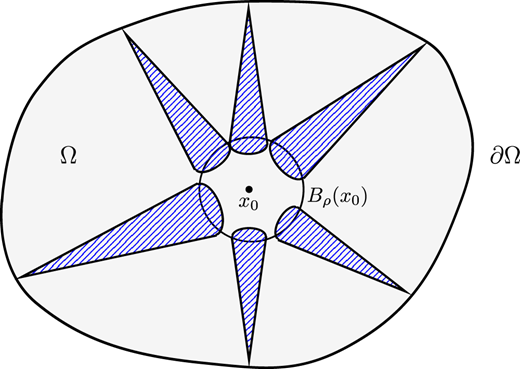
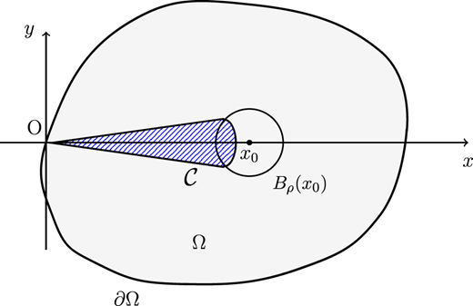
For any $t0∈[T0,T*)$⁠, let $x0∈Ω$ such that $u(x0,t0)>0$⁠. Since u is continuous, there exists a ball $Bρ0(x0)⊂Ω$ with center $x0$ and radius $ρ0>0$ and a positive number $δ0$ such that $u>0$ in $Bρ0(x0)×(t0,t0+δ0)$⁠. To proceed our argument, we will work under the polar coordinates around any boundary point of $Ω$⁠. Let $x1$ be any point on $∂Ω$⁠. By a translation, let $x1$ be transformed to the origin. We use the polar coordinates around the origin, where Eqn (1.1) is invariant under a parallel transformation and a rotation and thus, if necessary, by the rotation around the origin, we may assume that the first component axis is the line passing through two points, the origin and $x0,$ and the other component axes are orthogonal to the above first axis and each other. Then, we make some conic space region with vertex at the origin and small angles around the first axis such that the final arc like part of the cone is in $Bρ0(x0)$⁠. This conic space region is denoted by $C$ and, let $R:=C×(t0,t0+δ0).$ It is verified by the convexity of the domain that $C⊂Ω,$ if the angles around the first axis are small, and thus, $ℛ⊂Ω×[T0,T*)$ for a small positive $δ0$⁠.

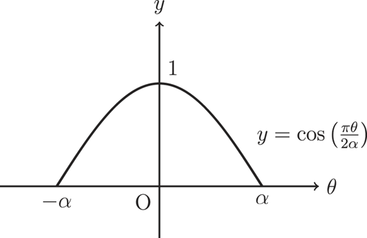
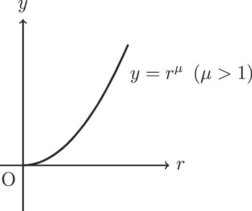
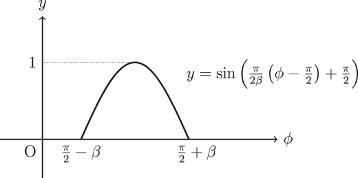
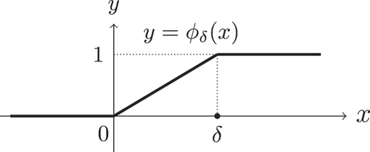
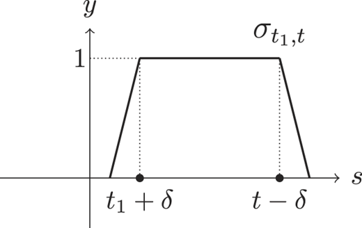
Let the comparison function in the three dimension be defined as

in the time-space region $ℛ:=C×(t0,t0+δ0)$ given by the variables $(r,θ,φ,t)$ in the range

where the positive parameters $α,β,δ0,mandμ$ are determined according to the demand, later. As before, we choose $α,β$ and $δ0$ so small that $ℛ⊂Ω×[T0,T*)$⁠. Again, that is possible by the hypothesis that the domain $Ω$ is convex (see Figures 3–5).

For brevity, we use the abbreviation hereafter

There holds

We know that

where

The drift term is computed as

and thus,

if we choose as $μ22≥(π2β)2$ which is verified by a large positive $μ$ depending on a small $β$⁠, and the lower positive bound of $sinφ$ such that $12≤sinφ≤1$ for $φ∈(π2−β,π2+β)$⁠.

and thus, letting $Lw=∂twq−Δpw$⁠, we have

Here the reasoning is as follows: since $0≤r≤R=diam(Ω)andt0≤t≤t0+δ0$⁠, the parameter m can be so small that the quantity in the bracket is positive. Thus, $Lw=∂twq−Δpw≤0=Lu$ in $ℛ$⁠. The boundary condition of w is verified as follows: On the lateral boundary, $w=0$ because at $θ=α,−α,$

and at $φ=π2−β,π2+β$⁠,

On the arc like boundary of $ℛ,w≤u$ if the parameter m is so small that $0≤w≤mδ0(diam(Ω))μ≤minAu$⁠, where $A=Bρ0(x0)×(t0,t0+δ0).$ On the initial boundary $C×{t=t0},w(x,t0)=0≤u(x,t0)$⁠. Therefore, w is the subsolution of L in $ℛ$ and thus, $u≥winℛ$ by Theorem 3.3. Hence, the solution u is positive in $ℛ.$ This is true for any $ℛ$ with vertex on the boundary $∂Ω$ and thus, u is positive in $Ω×(t0,t0+δ0)$⁠, because of the convexity of the domain. Hence the proof is complete. □