Benchmarking token mixers for efficient transformer-based learned video compression

Video compression is fundamental to modern digital infrastructure, balancing the critical trade-off between visual fidelity and bandwidth reduction. While conventional codecs rely on hand-crafted modules for motion estimation and residual coding (Bross et al., 2021; Sullivan et al., 2012; Xu and Liu, 2019), learned video compression (LVC) has emerged as a data-driven alternative, leveraging deep neural networks to model complex, non-linear spatio-temporal dependencies (Chen et al., 2024a; Jia et al., 2024). Early LVC frameworks, typically built on convolutional neural networks (CNN) and optical flow-based motion prior, have achieved impressive performance (Li et al., 2021; Lu et al., 2018). However, the local receptive fields of CNNs inherently limit their ability to capture global redundancies, a bottleneck that recent research attempts to circumvent by introducing increasingly complex auxiliary modules such as multi-scale priors and advanced feature-domain motion compensation (Jiang et al., 2024; Sheng et al., 2021, 2024; Yang et al., 2024).

The adoption of Transformer architectures, pioneered by the video compression transformer (VCT) (Mentzer et al., 2022), offered a promising solution to this limitation. By implicitly encoding tokenized frames and employing self-attention mechanisms, VCT captures long-range dependencies that CNNs miss without restricting the prior in the captured motions by optical flow algorithms. However, this global modeling comes at a steep drawback: the quadratic computational complexity of multi-head self-attention (MHSA) introduces substantial overhead (Vaswani et al., 2017). Subsequent studies have attempted to mitigate this by re-introducing complex motion contexts or hybridizing Transformers with heavy priors (Chen et al., 2023a, 2023b; Xiang et al., 2023). While these state-of-the-art (SOTA) methods achieve incremental coding gains, they create a significant knowledge gap: the rapid expansion of architectural complexity obscures the contribution of the core entropy coding mechanism. It remains unclear whether performance gains stem from the inherent power of the attention mechanism or simply from the increased parameter count and auxiliary priors. Furthermore, despite the impressive rate-distortion (R-D) performance of implicit-motion frameworks like VCT, their reliance on standard MHSA introduces a severe computational bottleneck. Specifically, the quadratic complexity $O(N2)$ of global MHSA with respect to the number of spatial tokens makes it prohibitively expensive for high-resolution video compression.

To address the aforementioned problems, we propose an abstracted transformer entropy model (ATEM). Our approach is inspired by the MetaFormer philosophy (Yu et al., 2021), which generalizes the vanilla ViT (Dosovitskiy et al., 2020) framework to demonstrate that the transformer architecture, rather than the specific attention mechanism, is the primary driver of performance in classification tasks. We hypothesize that the general macro-architecture of the transformer-based entropy model contributes more to compression performance than the specific attention mechanism itself. We utilize the seminal VCT architecture as a controlled testbed to isolate and rigorously evaluate the efficiency of the token mixer – both the primary driver of context modeling and contributor of computational overhead. Unlike previous works that chase SOTA performance via complex add-ons, our goal is architectural clarity and efficiency, because while LVC has achieved impressive R-D performance, high computational complexity remains a primary barrier to practical adoption. As emphasized in expert discussions (Chen et al., 2024b; Ling et al., 2022), there is an urgent industry demand for video coding solutions that prioritize low power consumption and interpretability over marginal gains in bit-rate. To do so, we systematically benchmark six distinct token mixers – defined as the core neural operators responsible for spatial or temporal feature aggregation across tokens – ranging from parameter-free pooling to hybrid convolution-attention mechanisms, aiming to answer whether the $O(N2)$MHSA is strictly necessary for latent entropy modeling, or if efficient token mixers can match this performance at a lower computational cost to identify the Pareto-optimal design for ATEM.

Our study yields critical insights into the performance of the entropy modeling in ATEM, as summarized in Figure 1. First, the significant performance degradation observed with parameter-free Pooling-Mixer confirms that implicit spatial context modeling is required for both reconstruction quality and bit saving, establishing a clear performance lower bound. Second, we find that spatial MLP modules (MLP-Mixer), despite their success in high-level classification tasks, are unsuitable for compression, incurring high computational costs without yielding coding gains. In contrast, introducing local inductive biases via Convolutional and Hybrid architectures with Attention-CNN/CNN-Attention mixed blocks (Conv-Mixer, Attn-Conv Hybrid Mixer, Conv-Attn Hybrid Mixer) proves highly effective for maximizing absolute reconstruction quality, albeit at the expense of increased model complexity. Ultimately, we demonstrate that the optimal balance is achieved by Sliding-Window Attention (Swin-Mixer); by restricting self-attention to local windows, this configuration eliminates redundant global computations, significantly reducing MACs while maintaining high-fidelity context modeling. The contributions of this paper are four-fold:

1. We propose a modular ATEM that decouples the token mixer from the entropy model. This establishes a rigorous methodology for isolating component-level efficiency contributions, independent of confounding variables like advanced quantization or motion priors.

2. We quantify the “cost of attention” by replacing MHSA with parameter-free pooling layers (Pooling-Mixer). We demonstrate that while pooling provides a baseline for structure preservation, it degrades coding efficiency by up to 12.56% in terms of BD-rate, proving that implicit context modeling is non-negotiable for video compression, unlike in high-level vision tasks where pooling can suffice.

3. We introduce a windowed attention configuration (ATEM-Swin) that outperforms the VCT baseline by up to −14.86% in BD-rate while simultaneously reducing computational complexity (kMACs/pixel) by 17.6%. This identifies the sliding-window mechanism as the optimal efficiency trade-off, superior to both full global attention and lightweight pooling.

4. We reveal that hybrid architectures (ATEM-Hybrid AC/CA) combining Convolution and Attention achieve the highest absolute quality, outperforming the baseline by up to −16.64%, at a small increased cost of 1.73%. This distinction between “Efficiency-First” (ATEM-Swin) and “Quality-First” (ATEM-Hybrid) designs provides clear guidelines for future low-complexity LVC development.

The remainder of this paper is organized as follows: Section 2 reviews the evolution of LVC, tracing the paradigm shift from residual coding to Transformer-based implicit modeling. Section 3 details the architecture of the VCT testbed, defines the proposed ATEM framework, and describes the design of the six token mixer variants. Section 4 presents data set specifications, experimental setups, and a comprehensive quantitative and qualitative analysis of the complexity-distortion trade-offs. Finally, Section 5 offers concluding remarks and discusses implications for future video coding standards.

The fundamental objective of video compression is to minimize spatio-temporal redundancy between frames. Traditional codecs, such as HEVC and VVC (Nguyen and Marpe, 2021), achieve this through a “predict-and-transform” paradigm: using block-based motion estimation to predict the current frame and subsequently coding the residual error. Early LVC frameworks adopted this blueprint directly. For instance, DVC (Lu et al., 2018) replaced the hand-crafted motion estimation and residual coding blocks with CNN, utilizing a learned optical flow network [e.g., SPyNet (Ranjan and Black, 2016)] to warp the previous frame and compressing the pixel-domain residual.

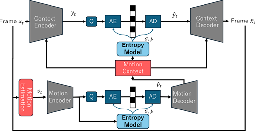
However, residual coding is inherently limited by its reliance on linear subtraction, which struggles to model complex, nonlinear dependencies as scenes in video media have been expanding rapidly. To address this, the LVC field shifted toward conditional coding, where motion information serves as a context to condition the prediction in entropy model rather than a subtraction target. DCVC (Li et al., 2021) pioneered this approach by introducing feature-domain motion compensation, refining motion information in the latent space to tighten the entropy bound. Subsequent frameworks have aggressively optimized this paradigm: recent SOTA methods utilize multiscale contexts, context-adaptive entropy models, sophisticated motion priors, and advanced frame encoder adapted from learned image compression works (Cheng et al., 2020; He et al., 2022; Liu et al., 2023) to significantly boost performance (Benjak et al., 2023; Chen and Peng, 2023; Li et al., 2023; Lu et al., 2023; Qi et al., 2023). The generalized framework of such design is illustrated in Figure 2. The process begins with the current input frame $xt$ at time $t$ and the previously reconstructed frame $x^t−1$⁠. A motion estimation module (⁠$ME$⁠) (using usually an optical-flow network) calculates the motion vectors (⁠$vt$⁠) representing the temporal displacement between these frames. Crucially, in these frameworks, this motion information is explicitly compressed into the bitstream: the $vt$ is processed by a motion encoder (⁠$Emv$⁠), quantized (⁠$Q$⁠), and arithmetically encoded (⁠$AE$⁠), before being reconstructed by the decoder as $v^t$⁠. Simultaneously, a motion context module (⁠$MC$⁠) refines the motion vectors to generate necessary contexts to aid the encoding and decoding process of the latent feature $yt$ and $y^t$⁠. The motion context is also the key prior to predict the probability mass function (PMF) in the entropy model. The predicted means $μ$ and scales $σ$ are fed into arithmetic coders for compressing the latent into the bitstream (⁠$AE$⁠) and vice versa (⁠$AD$⁠). While effective, these improvements come at the cost of increasing architectural complexity. Most conditional coding pipelines remain heavily reliant on off-the-shelf optical flow networks (Ranjan and Black, 2016) – a handcrafted prior that may not generalize to complex motion patterns. Furthermore, the reliance on CNN backbones limits the global receptive field both during context modeling and motion prior refinement, necessitating deeper networks or iterative refinement steps that complicate the network design (Chen et al., 2025; Phung et al., 2025).

To overcome the locality limitations of CNNs and the dependency on motion priors, Transformer-based architectures have emerged as a powerful alternative. We categorize these designs as frame-implicit frameworks, distinguishing them from the motion-centric approaches in two key ways.

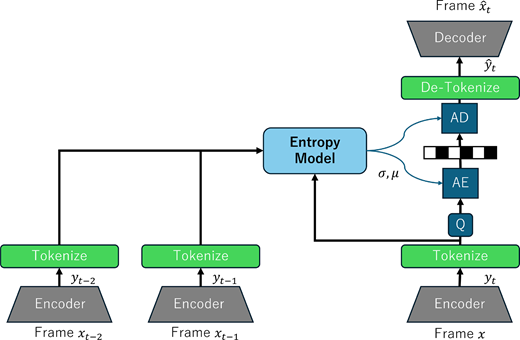
First, these frameworks abandon the separate hyper-prior stream for local context modeling in favor of implicit self-attention mechanisms. Second, they eliminate dedicated optical flow networks. Instead of warping features based on estimated motion vectors, the temporal context is implicitly learned via attention layers. The VCT (Mentzer et al., 2022) pioneered this direction (a generalized framework of its frame implicit design is illustrated in Figure 3). This framework performs the core encoding operations predominantly within a latent feature space in a streamlined, single-profile approach. Initially, a spatial encoder extracts and downsamples the current frame $xt$ into the latent space before each frame is tokenized into a sequence of tokens (each pixel is represented by one token). At each encoding step, previously reconstructed latent tokens $y^t−1$ and $y^t−2$ (stored in a buffer) are viewed as the condition to predict the PMF of the current tokens $yt$ by the transformer-based entropy model. Motion estimation is completely absent as the temporal context is based on concatenated token sequence from two previous encoded frames. VCT utilizes MHSA to capture global spatial dependencies within the current frame, and employs a cross-attention module to query temporal information from previously transmitted latents, which also undergo separate and joint MHSA layers for intra and inter-frame context modeling.

This design theoretically offers a “clean slate” for video compression, as the temporal context is not bottlenecked by the accuracy of an optical flow estimator. However, the standard VCT implementation incurs high computational costs due to the quadratic complexity of global attention (⁠$O(N2)$⁠). While VCT demonstrated that Transformers can work for compression, subsequent studies have often reverted to adding complexity [e.g., combining Transformers with motion priors (Chen et al., 2023b; Xiang et al., 2023)] to chase performance gains. In contrast, this work revisits the pure Transformer architecture to rigorously evaluate the efficiency-distortion trade-off of the entropy model itself.

To rigorously evaluate the efficiency of different token mixers, we adopt the VCT (Mentzer et al., 2022) as our foundational baseline. VCT employs a purely Transformer-based entropy model to predict the probability distribution of quantized latent features, replacing the handcrafted motion prediction loops of traditional codecs.

The pipeline begins by processing input frames through a standard encoder (He et al., 2022) to generate quantized latent representations $y^$ with dimensions $[192,H/16,W/16]$⁠. A key characteristic of this stage is that frames are processed independently to generate primary feature maps. This step is essential for obtaining a discrete representation of the frames, as the encoder learns to transform high-resolution input images into compact yet informative latent codes. Bridging the quantization step and the entropy coder is a window-based tokenization module (often referred to as the “patcher”). This module converts 2D feature maps into token sequences by dividing the latents of the current and previous frames into smaller blocks. Standard VCT implementations utilize a nonoverlapping sliding window strategy to partition the input map, where each token represents a single spatial location with a 192-channel vector. However, to leverage temporal redundancy, the context extraction mechanism employs a larger, overlapping window when accessing previous frames. For instance, the VCT baseline configuration employs a $4×4$ token grid for the current frame, expanding to an $8×8$ search window for previous frames to effectively model redundancy within larger areas.

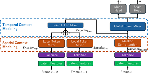
The core of VCT is its Transformer-based entropy model. This model is responsible for predicting the Gaussian parameters (mean $μ$ and scale $σ$⁠) required for losslessly compressing the latent features via arithmetic coding. The architecture integrates three critical design components, which serve as the control variables for our study: Intra Frame Context (Encoder-Masked): A mechanism to model local spatial dependencies within the current frame. Inter Frame Context (Cross Attention): A temporal mechanism that extracts context from the two preceding frames (⁠$t−1,t−2$⁠) and fuses this information with the current latent representation. Temporal Context Modeling (Encoder-Sep and Encoder Joint): Additional modules for further refine latent from previous frames. The synergy between these components allows for efficient compression while maintaining rich contextual information critical for high-quality reconstruction.

In this paper, we propose to abstract especially the transformer-based core entropy model (ATEM). This abstraction allows for a granular analysis of how specific components contribute to the performance-efficiency trade-off.

While the attention mechanism (Vaswani et al., 2017) is often credited as the primary driver of Transformer performance, recent studies like MetaFormer (Yu et al., 2021) suggest that the general architecture, specifically the sequence of token mixing and channel mixing, plays a more significant role. Inspired by this, we hypothesize that a Transformer-based LVC framework should be adaptable to arbitrary token mixers, with performance scaling according to the mixer’s inductive bias (e.g., local vs global). A more thorough understanding can be obtained by dividing the entropy into two processes:

Spatial context modeling: In the baseline VCT architecture, spatial modeling is distributed across two distinct stages. First, the spatial encoder (⁠$EncoderSep$⁠) extracts spatial features from the quantized latents of reference frames. To balance local feature extraction with computational complexity, this block typically operates on $8×8$ token patches using six layers of MHSA. Second, the contextual decoder fuses these features with the current frame’s tokens to predict the final probability distribution.

Spatial context modeling is critical for exploiting local redundancies; however, its implementation differs significantly between the reference and current branches. Within the contextual decoder (processing the current frame), strict causality must be enforced to maintain the autoregressive property – ensuring that the prediction of the current token $y^t$ relies solely on previously decoded tokens. Consequently, VCT implements a masked self-attention block here (⁠$EncoderMasked$⁠).

In the ATEM framework, we specifically focus our architectural exploration on $EncoderSep$⁠, which processes previous latents to generate reference features. We isolate this module because it allows for noncausal, bidirectional context modeling. Conversely, we keep the decoder’s spatial modeling fixed. Although recent works have proposed advanced causal schemes such as masked image modeling (MIM) or improved masked CNNs (Koyuncu et al., 2022; Mentzer et al., 2023; Qian et al., 2022), ATEM restricts the decoder to the vanilla masked MHSA. This ensures that our comparisons remain fair and strictly isolate the efficiency gains of ATEM.

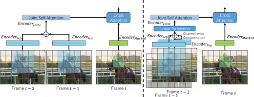
Temporal context modeling: The temporal context model is responsible for reducing inter-frame redundancy, effectively replacing the explicit motion estimation modules found in traditional conditional codecs. In the baseline design, this is achieved through a combination of joint self-attention (⁠$EncoderJoint$⁠) and cross-attention (Global Token Mixer).

To predict the current frame $f^i$⁠, the model retrieves latent features from the two previously reconstructed latents (⁠$f^i−1,f^i−2$⁠). These historical latents are concatenated to form the Key (⁠$K$⁠) and Value (⁠$V$⁠) pairs for the cross-attention block, while the current frame’s spatial features serve as the Query (⁠$Q$⁠). This mechanism allows the model to implicitly query relevant temporal information – such as object displacements and motion trajectories – without relying on explicit optical flow warping.

For Intra-frame (I-frame) coding, where no reference frames exist, the model relies exclusively on spatial context, resulting in the higher bit-rates characteristic of I-frames. This behavior is consistent with both traditional standards like HEVC (Sullivan et al., 2012) and modern LVC frameworks like DCVC (Li et al., 2021). Temporal context modeling is the defining characteristic that distinguishes video compression from image compression, as the effective utilization of temporal priors can reduce the rate cost for the current frame by a significant margin. In the ATEM framework, we specifically analyze this trait by decomposing the architecture into a joint frame module (for reference processing) and a cross-attention mixing module (for temporal fusion).

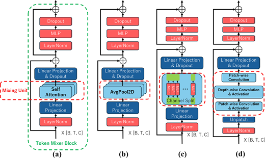
To systematically investigate the efficiency-distortion trade-off within the ATEM framework, we implement and evaluate four distinct categories of token mixers, selected to span the architectural spectrum from parameter-free operations to complex global modeling. As illustrated in Figure 4, ATEM targets the Local Token Mixer, Joint Token Mixer, and Global Token Mixer modules to quantify their specific roles. We replace the vanilla MHSA blocks (default token mixer in transformer architecture) within the spatial encoder (⁠$Encodersep$⁠) with each candidate token mixer to evaluate intra-frame efficiency. We apply a similar substitution to the joint context encoder. Crucially, to accommodate sliding window-based token mixers in the temporal domain, we modify the baseline architecture from sequence-wise to channel-wise latent concatenation and replace the dedicated cross-attention module with the target token mixer. These adaptations unify the interface for spatial and temporal modeling, allowing for a direct comparison of mixer efficiency. As summarized in Table 1, the six distinct token mixers we benchmarked span from parameter-free operations to complex hybrid modeling. The specific architectural details and inductive biases of each are elaborated in the subsequent subsections with their detailed layouts shown in Figure 5.

Inspired by MetaFormer, we hypothesize that the general architecture of the Transformer contributes more to performance than the specific attention mechanism. To test the theoretical lower bound of LVC efficiency, we replace the vanilla MHSA blocks with simple pooling layers. This substitution removes all data-dependent spatial interaction, leaving only fixed, local aggregation.

In MetaFormer (Yu et al., 2021), the pooling operation was proposed as the simplest “Token Mixer” capable of validating this architectural hypothesis. We adopt this intuition to establish a baseline for ATEM. While subsequent study (Yu et al., 2022) has explored even simpler Identity mappings (where the token mixer is effectively removed) for classification tasks, we determine this approach is unsuitable for video compression. Unlike classification tasks where global semantics can sometimes survive without implicit mixing, compression requires the rigorous modeling of local spatial probabilities. Identity layers isolate tokens, allowing the subsequent MLP to operate only channel-wise, which destroys the spatial context required for entropy minimization. Therefore, we utilize pooling as the minimal viable mixer.

The standard MHSA mixer computes global dependencies via:

This operation requires calculating an $N×N$ attention map, leading to quadratic complexity $O(N2)$⁠. In contrast, the simple Pooling-Mixer replaces this with a parameter-free local aggregation:

where $k$ is the kernel size. This reduces the computational complexity to linear $O(N)$⁠, serving as the efficiency lower-bound.

We next investigate whether fixed-topology networks – architectures that rely on static weights rather than content-adaptive attention maps – can replace dynamic attention. To this end, we examine two representative architectures: MLP-Mixer and Conv-Mixer.

Originally proposed for classification (Touvron et al., 2021), this architecture replaces self-attention with a multilayer perceptron that mixes information across channels within tokens. While this eliminates the overhead of calculating dynamic attention maps, we investigate its suitability for compression. Unlike classification tasks, which prioritize semantic invariance (often discarding spatial precision), video compression demands pixel-perfect reconstruction – a requirement that may struggle against the rigid connectivity of a fixed MLP.

Second, recognizing that visual redundancy is often highly localized, we implement Conv-Mixer, a pure CNN-based token mixer. By replacing global attention with depth-wise convolutions, we target local spatial redundancy independently within each latent channel. This tests the hypothesis that standard CNN receptive field is also sufficient in this scenario given ATEM structure contributes more to the entropy modeling ability.

To further improve the context modeling ability of ATEM, we investigate Hybrid Architectures ATEM-Hybrid AC and ATEM-Hybrid CA. Their structure design is illustrated in Figure 6(a) and (b). It is well-established that CNNs excel at capturing high-frequency local details; however, their receptive field is inherently limited by fixed kernel sizes and strides. Conversely, self-attention mechanisms are superior at modeling long-range dependencies, granting the model global perception of the frame. Yet, this comes at a significant cost: MHSA suffers from quadratic computational complexity and, due to its patch-based processing, can sometimes fail to preserve fine-grained local textures – a limitation often masked by its success in high-level semantic tasks like classification.

By combining convolutional with self-attention blocks as token mixers, we aim to leverage the complementary inductive biases of both architectures. While previous work (Yu et al., 2022) has successfully explored this synergy in classification tasks, its application specifically within entropy modeling remains under-explored. We hypothesize that this hybrid approach will yield the highest coding efficiency (lowest BD-rate) by effectively modeling both local texture details and global motion patterns, albeit at the expense of increased computational cost.

To alleviate the $O(N2)$ complexity bottleneck identified in the introduction, we adopt the windowed (W-MSA) and sliding-window (SW-MSA) attention mechanisms from the Swin-transformer (Liu et al., 2021). While the broader computer vision literature offers numerous efficient attention variants – including linear approximations [e.g., Linformer (Wang et al., 2020), Performer (Choromanski et al., 2020)], sparse attention patterns [e.g., Longformer (Beltagy et al., 2020)], and channel-wise attention [e.g., Hydra Attention (Bolya et al., 2022)] – our framework specifically targets token mixers that enforce spatial locality. Many linear and sparse variants are designed to approximate global context at a reduced computational cost. However, as our subsequent evaluations will demonstrate, global context is largely redundant for latent entropy modeling. Instead, architectural operators that inherently preserve local spatial inductive biases, such as convolutional layers and window-based attention, are far more critical for efficiently compressing high-frequency residual textures.

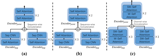
As shown in our implementation in Figure 6(c), we pair windowed attention with sliding-window attention to enable cross-window interaction while maintaining linear complexity relative to the image resolution. This design partitions the latent frame into non-overlapping local windows, restricting attention operations to local neighborhoods, while the cyclic shifting in SW-MSA re-establishes cross-window connections in subsequent layers. This strategy reduces computational complexity from quadratic to linear (⁠$O(N)$⁠), offering the optimal balance between long-range modeling and efficiency. We configure the window size to $2×2$ for the spatial patches (within the $4×4$ grid) and $4×4$ for the temporal patches (within the $8×8$ grid).

Beyond the spatial domain, we identified a specific inefficiency in the baseline VCT temporal module. The vanilla VCT models temporal context by concatenating spatial tokens from two reference frames along the sequence dimension (⁠$2×T$⁠), resulting in a joint attention matrix of size $O((2T)2)$ (i.e., $1282$⁠). To resolve this and enable the use of efficient windowed attention in the temporal domain, we propose a streamlined Channel-Concatenated Temporal Mixer. Instead of increasing the sequence length, we concatenate the historical contexts of the two previous frames along the channel dimension (depth-wise) and apply a linear projection to restore the original channel depth (⁠$C=768$⁠).

This “overlay” approach is guided by the intuition that stacking adjacent frames depth-wise allows the model to detect local changes more directly. Crucially, this modification reduces the effective sequence length back to $T$ (64 tokens). Consequently, the complexity of the joint attention matrix is reduced from $O(1282)$ to $O(642)$⁠, and the subsequent cross-fusion matrix is reduced from $O(1922)$ to $O(1282)$⁠. This reduction is critical for achieving the lowest computational cost of our proposed ATEM-Swin configuration. A comparison between the original approach and our optimized version is demonstrated in Figure 7.

We utilize the Vimeo-90K data set (Xue et al., 2017) for training the LVC model. Following standard LVC evaluation protocols, we benchmark our method on the UVG (Mercat et al., 2020), MCL-JCV (Wang et al., 2016), and four HEVC data sets – Class B through E (Bossen, 2010).

The UVG data set contains seven video clips at $1920×1080$ pixels in spatial resolution and 120 frames per section in temporal resolution.

The MCL-JCV data set contains 30 video clips with the same 1080p resolution but are varied in 24, 25 and 30 FPS, offering a diverse range of motion characteristics.

The four HEVC data sets have varied resolution and unique traits: Class B has five videos in $1920×1024$ pixels; Class C has five videos in $832×448$ pixels; Class D has four videos in just $416×240$ pixels; Notably, Class E at $1280×720$ pixels features static conference scenes characterized by stationary backgrounds and minimal foreground motion.

Data pre-processing: While traditional codecs (HEVC, VVC) operate in the YUV420 color space, the LVC community predominantly utilizes RGB data to leverage off-the-shelf feature extractors. Consequently, we convert the original YUV420 source files into individual RGB444 PNG frames using the standard BT.601 conversion matrix. During testing, sequences are partitioned into segments (Group of Pictures) of 32 frames each.

We follow standard learned compression practices and minimize a R-D objective using a Lagrange multiplier $λ$⁠. The loss function is formulated as:

where $yi^$ is the quantized latent features, and $D(x,x^)$ represents the distortion metric, evaluated using mean squared error (MSE). To enable end-to-end backpropagation through the quantization step, we utilize straight-through estimation during training, and standard rounding during inference.

For training, we keep the hyper-parameter the same across all token mixer configurations. The original frame at resolution of $256×256$ is encoded and quantized by the ELIC frame encoder (He et al., 2022) to latent shape of $[16,16,192]$⁠. The patcher and embedding layers further divide them into several $4×4$ patches and embedded to $768$ channels. The ATEM’s hidden dimension is $768$ throughout different token mixers. For feedforward layers in all token mixers, the MLP expansion size is set to 4. Training is done with 1M steps at learning rate of $1×10−4$ for the one initial $λ=0.01$ (MSE). Subsequently, we fine-tune separate models for different $λ$ values for an additional 200k steps at a reduced learning rate of $1×10−5$⁠. When training on the Vimeo-90k data set using a distributed setup with two NVIDIA RTX 3090 GPUs, it takes approximately 5 days to complete the first $λ$⁠. To generate the full R-D curve, models for subsequent $λ$ values are initialized with the converged base model weights and fine-tuned, reducing the training time to approximately 1 day per additional rate point.

In our evaluation framework, we apply the selected token mixer symmetrically to both the spatial and temporal context encoders. While an asymmetric ablation (e.g., replacing only the spatial mixer) might theoretically isolate dimensional contributions, we deliberately enforce architectural homogeneity for two reasons. First, mixing fundamentally different inductive biases across dimensions creates confounding variables, obscuring the intrinsic representation capability of the evaluated mixer. Second, because the baseline context model relies on $O(N2)$ Global Attention, retaining it in either dimension would act as an asymptotic computational bottleneck. This would artificially mask the $O(N)$ efficiency gains of lightweight modules like Swin-Mixer or Conv-Mixer. Therefore, symmetric replacement is strictly necessary to accurately measure both the true efficiency lower bound and the holistic R-D impact of the target operator.

It is important to note that the Masked-MHSA module within the autoregressive entropy bottleneck remains fixed across all ATEM configurations. This is a strict structural constraint: the Masked-MHSA enforces the causality required for stepwise decoding (⁠$tn$ conditioned on $t1,…,tn−1$⁠). The alternative token mixers evaluated in this study (e.g., convolution, sliding-windowed self-attention) are inherently bidirectional. Consequently, they cannot be substituted into the autoregressive loop without fundamentally violating either the decoding causality or their own structural inductive biases.

Directly comparing the absolute R-D performance of different token mixer configuration against SOTA models in recent years [e.g., MCRT (Chen et al., 2023a), DCVC-FM (Li et al., 2024), DCVC-RT (Jia et al., 2025)] is confounded by the significant architectural differences in motion estimation, hyper-prior design, and entropy coding that have evolved since the original VCT. Our goal is not to propose a new SOTA system, but to isolate and evaluate the efficiency of the ATEM itself. Therefore, we strictly utilize the VCT architecture as a controlled testbed. This ensures that any observed performance gains or efficiency improvements are solely improved by the token mixer design, rather than unrelated enhancements in motion compensation or quantization. The insights derived here regarding the redundancy of global attention are architectural principles that can likely be transferred to reduce the complexity of modern SOTA transformer backbones (Chen et al., 2023b; Xiang et al., 2023).

Furthermore, while generative coding approaches have recently been adapted for LVC (Chen et al., 2021; Gao et al., 2025), they operate on a fundamentally different paradigm that prioritizes perceptual realism over the MSE fidelity targeted in this study. Consequently, we exclude these generative models from our current fidelity-based benchmark. However, we recognize the strategic importance of this domain; as highlighted in recent surveys (Ma et al., 2025), integrating priors from MIM offers a critical pathway to overcome the saturation of traditional distortion-oriented metrics – a promising direction we identify for future integration into the ATEM framework.

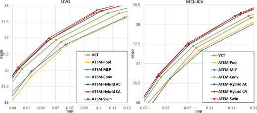
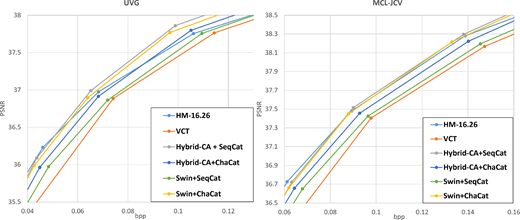
For quantitative comparison, we evaluate compression performance using R-D curves and BD-rate. Note that since the original VCT study did not benchmark on the HEVC test sequences, we trained our own VCT model from scratch with the same scheme used for ATEM as the baseline for fair comparison. The results are shown in Figure 8. As expected, the parameter-free Pooling-Mixer performs the worst, establishing the baseline for minimal spatial context modeling. Despite its higher parameter count and computational cost, MLP-Mixer yields negative gains relative to the VCT baseline. This stands in stark contrast to its success in high-level classification tasks, yielding our first major insight: inductive bias for locality is non-negotiable in entropy modeling. Unlike semantic tasks, compression requires pixel-precise modeling of high-frequency spatial residuals, which the rigid, global connectivity of MLPs fails to capture efficiently. Conversely, the convolutional mixer performs on par with the vanilla attention module. This validates our locality hypothesis: while global context provides secondary benefits, the core spatial dependencies required for accurate probability estimation are highly localized. Consequently, pure global, static connectivity in Spatial-MLP token mixer wastes parameter capacity on modeling irrelevant long-range correlations. Without the dynamic weighting of self-attention or the localized kernel of convolutions, Spatial-MLP fails to converge on high-frequency details, ultimately losing the latent representation and degrading R-D performance. Similar performance between ATEM-Conv and VCT also proves that the general macro-architecture of ATEM contributes more to the overall compression performance than the specific use of self-attention. Furthermore, the two hybrid architectures, ATEM-Hybrid AC and ATEM-Hybrid CA, outperform single-mode baselines, confirming the synergy between convolutional local biases and attention-based global modeling. Notably, Hybrid-CA (CNN$→$ Attention) achieves a 3.01% BD-rate advantage over the reverse order. This reveals a critical architectural principle: Local feature priming stabilizes global attention. We theorize that the initial CNN layer effectively extracts and aggregates sharp local edges, creating a robust, high-frequency feature representation that prevents the subsequent attention module from over-smoothing the latent space. On the contrary, the Attn-Conv Hybrid Mixer applies global attention first to un-primed patches, which tends to over-smooth the high-frequency residual signals globally, permanently degrading the fine-grained details required for optimal entropy minimization. Finally, the ATEM-Swin configuration achieves the optimal Pareto-frontier balance. By restricting attention to sliding windows, it enforces the necessary locality bias and minimizes computation, matching the high performance of the hybrid models at a significantly lower computational cost. Table 2 presents the BD-rate calculations of all proposed token mixers relative to the original VCT baseline, as it represents the foundational architecture for this class of Transformer-based LVC models.

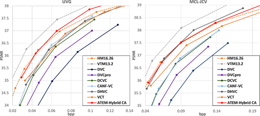
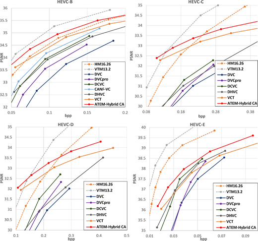
To broaden the comparison in the LVC landscape, we also compare the best-performing ATEM (equipped with the Conv-Attn Hybrid Mixer) against traditional codec testing suites HM-HEVC (JVET/HM, 2024), VTM-VVC (VCGIT, 2024), and pioneering LVC methods – including DVC (Lu et al., 2018), DVC-pro (Lu et al., 2020), DCVC (Li et al., 2021), DHVC (Lu et al., 2023), and CANF-VC (Ho et al., 2022) – on the UVG, MCL-JCV, and four HEVC data sets (Figures 9 and 10). Newer SOTA frameworks such as ST-XCT (Chen et al., 2023b) and MIMT (Xiang et al., 2023) are deliberately excluded from this specific ablation, as their architectures diverge significantly from the baseline VCT design (e.g., utilizing different hyper-priors or quantization schemes), which would confound our isolation of the token mixer’s contribution. Note that while the proposed ATEM models (e.g., ATEM-Hybrid) maintain a substantial performance margin over models like HEVC and DHVC on the UVG data set, this advantage narrows on the MCL-JCV data set, particularly in high-bitrate regimes. The primary driver of this discrepancy is the difference in temporal resolution and the resulting magnitude of inter-frame motion. The UVG data set predominantly consists of high-frame-rate sequences (up to 120 fps), which are characterized by dense temporal correlation and highly predictable, sub-pixel inter-frame displacements. In contrast, the MCL-JCV data set features standard cinematic and broadcast frame rates (ranging from 24 to 30 fps), resulting in significantly larger and more complex inter-frame motion vectors. This is also one of the reasons that the VTM-13.2 anchor continues to outperform the LVC-based variants. Traditional video codecs utilize highly optimized, variable-block-size motion estimation algorithms with expansive search ranges, allowing them to robustly capture large, discrete displacements. Conversely, the underlying motion estimation module inherited from our VCT baseline relies on implicit motion interpretation. While effective for dense temporal sampling, it struggles to accurately model large geometric deformations and fast motion at high bitrates where texture fidelity is paramount. Consequently, while the proposed ATEM token mixers drastically improve spatial and temporal entropy modeling efficiency, addressing the motion compensation bottleneck for low-framerate, high-motion content remains an orthogonal challenge for future LVC architectures.

While UVG and MCL-JCV (1080p) serve as standard benchmarks, our evaluation on the diverse HEVC data sets reveals critical insights into how resolution and content type affect learned compression. As shown in Figure 10, on Classes B, C and D, we observe that as video resolution decreases, the performance gap between LVC models and traditional codecs widens. Furthermore, all LVC models perform poorly on Class E (conference scenes with static backgrounds). This exposes a fundamental architectural flaw in the current learned quantization paradigm: The lack of dynamic spatial routing. Unlike traditional codecs (HEVC/VVC) that utilize specific modes to entirely bypass static regions, current dense LVC models process the entire frame uniformly. The feature extractor and token mixers continue to allocate channels and computational FLOPs to temporally redundant backgrounds. Therefore, one of the routes for future LVC frameworks is the necessary integration of sparse computation or token-pruning mechanisms to dynamically bypass static content.

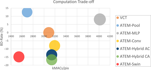
A critical evaluation of compression framework involves analyzing the trade-off between its R-D performance and its computational complexity. Table 3 details the specific metrics used for this assessment, including BD-rate (calculated on the UVG data set), computational cost (kMACs/pixel) and total parameter count.

The baseline VCT is well-known for its high computational demand, a trait confirmed by our measurements. In contrast, the Pooling-Mixer generally serves as the lower bound for complexity by eliminating learnable parameters and substituting complex attention operations with simple aggregations. On the other end of the spectrum, the MLP-Mixer exhibits the highest computational cost among all six implementations due to its dense, global connectivity; however, as previously discussed, this increased parameter load fails to translate into improved compression performance.

The hybrid models maintain a computational cost similar to the baseline – achieved by replacing half of the attention layers with convolutions while retaining the feed-forward blocks – yet they deliver significant performance gains. Finally, the ATEM-Swin configuration, which combines windowed and sliding-window attention, significantly reduces the size of the attention matrix while preserving global perception. This approach achieves the lowest MACs/pix and the optimal performance-efficiency trade-off. Note that due to the implementation of the channel-stacking method for past latent concatenation (Figure 7), ATEM-Swin configuration is able to achieve lower computational cost than ATEM-Pool.

In addition, to evaluate the practical applicability of the proposed architectures beyond theoretical MACs/pix, we benchmarked the actual encoding and decoding latency (seconds per frame) for 1080p sequences on an NVIDIA RTX 3090 GPU (Table 3). The empirical runtimes closely align with our theoretical complexity analysis and reveal two distinct deployment paradigms. First, the ATEM-Swin configuration achieves a profound $∼$50% reduction in both encoding (1.11 s) and decoding (0.46 s) times compared to the VCT baseline (2.13 and 1.08 s, respectively). This hardware-level speedup confirms that combining channel-wise temporal concatenation with $O(N)$ windowed attention effectively alleviates the computational bottlenecks associated with MHSA, making it highly suitable for low-latency applications. Conversely, the top-performing ATEM-Hybrid CA maintains computational parity with the baseline’s runtime while delivering a 16.64% BD-rate reduction. This demonstrates that the re-introduction of localized convolutional priors (Conv $→$ Attention) drastically improves latent feature representation without incurring a real-world latency penalty, presenting an optimal solution for quality-prioritized offline encoding.

To rigorously isolate the contribution of our proposed channel-wise temporal concatenation, we conducted an ablation study comparing it directly against the traditional sequence-wise concatenation used in the VCT baseline. We evaluated this across our top-performing hybrid (ATEM-Hybrid CA) and lightweight sliding-window (ATEM-Swin) token mixers. The results, detailing both R-D performance and computational cost in Tables 4 and 5, yield two critical architectural insights.

The primary driver of macro-level efficiency in the ATEM framework is the channel-wise concatenation strategy. Sequence-wise fusion concatenates Frame $t−2$ and Frame $t−1$ along the spatial sequence dimension, doubling the token count (⁠$N→2N$⁠). Because context-modeling complexity scales nonlinearly with sequence length, this causes a computational explosion. As observed in our data in Table 4, reverting the ATEM-Swin model to sequence-concatenation incurs a massive penalty of approximately 500 kMACs/pix. By stacking temporally adjacent frames along the channel depth dimension instead, ATEM maintains a strict $O(N)$ sequence length, decisively lowering the computational floor. Furthermore, it should be noted that in transformer-based LVC frameworks, the local and joint context encoders (local and joint token mixers) are executed only once per frame to extract past information. In contrast, the autoregressive entropy model must be queried iteratively (typically 16 times per frame) during the stepwise decoding of the current latents. Because this autoregressive loop acts as a computational multiplier, reducing the overall token sequence length via channel-wise concatenation yields a substantially greater reduction in both theoretical computational cost and empirical inference latency than optimizing the asymptotic complexity of the token mixers alone.

Beyond computational cost, the concatenation strategy fundamentally impacts performance depending on the token mixer’s inductive bias: As shown in Figure 11, when ATEM-Swin is forced to use sequence-concatenation, its compression performance severely degrades, regressing to near-baseline level. This occurs because extending the sequence length disrupts the 2D spatial grid topology. Consequently, sliding windowed attention erroneously mixes spatial neighbors with temporal boundaries, destroying their localized inductive bias. Thus, channel-wise concatenation is strictly mandatory for ATEM-Swin to function effectively. Interestingly, the ATEM-Hybrid CA achieves slightly higher R-D performance with sequential concatenation than with channel concatenation. Because its hybrid layers still retain the global attention layers, it is permutation-invariant and benefits from having explicit, separated temporal tokens (⁠$2N$⁠) rather than projecting them into a squeezed channel dimension.

Ultimately, this ablation demonstrates that while global models can theoretically leverage sequence-wise temporal fusion for maximum quality, channel-wise concatenation remains the optimal, and often strictly necessary, strategy for building highly efficient LVC frameworks.

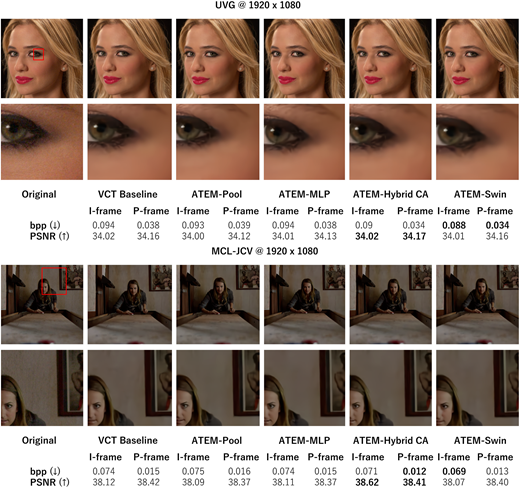
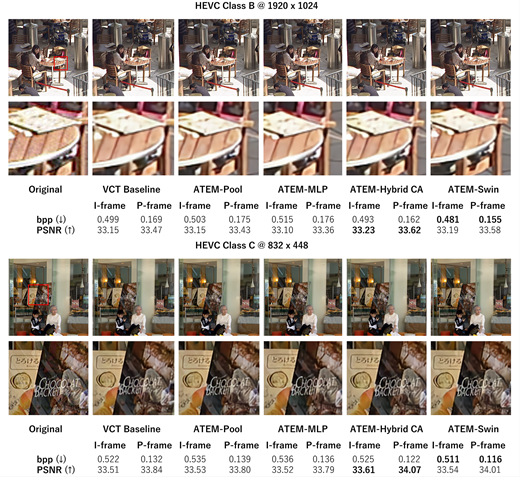
Figures 12 and 13 present qualitative comparisons of the reconstructed I-frames and P-frames across different token mixer configurations. First, from a perceptual standpoint, the hybrid and localized architectures (such as ATEM-Hybrid and ATEM-Swin) exhibit vastly superior preservation of high-frequency local patterns and sharp edges compared to the VCT baseline and MLP-Mixer. This visually confirms the necessity of localized inductive biases for pixel-precise texture reconstruction. Second, the true efficacy of the temporal context model is revealed by the compression gap between the I-frame and the subsequent P-frame. For this analysis, we report metrics for the first frame (I-frame) and the third frame (P-frame), as the third frame is the first to fully benefit from the two-frame temporal context window (⁠$t−1,t−2$⁠). This comparison emphasizes the model’s ability to exploit temporal redundancy. We observe significant disparities in rate reduction capabilities: The lower bound Pooling-Mixer model only reduced the rate cost by 58%, 78%, 65% and 74% on the UVG, MCL-JCV, Class B and C data sets, while the best performing ATEM-Hybrid CA significantly improves temporal exploitation, achieving reductions of 62%, 83%, 67% and 77%. The most efficient ATEM-Swin model also achieved 61%, 81%, 68% and 77% in this metric. This profound inter-frame bit savings, achieved without degrading perceptual quality, underscores the primary advantage of the proposed token mixer modifications.

Based on our comprehensive benchmarking through different perspectives, we distill the following key insights: (1) Purely global, static modules like the MLP-Mixer are ineffective for residual entropy coding. Structural inductive biases for spatial locality (such as convolutions or windowed attention) are mandatory for preserving high-frequency textures. (2) In hybrid architectures, the order of operations matters. Applying convolutional layers before global attention (Conv-Attn) significantly outperforms the reverse order by extracting stable edges before global mixing. (3) The Swin-Mixer achieves the Pareto-optimal balance, delivering SOTA R-D performance while maintaining a strictly linear $O(N)$ computational complexity. (4) Channel-wise temporal concatenation is a strict structural prerequisite for any architecture utilizing localized token mixers, as it preserves the 2D spatial grid topology that sequence-wise concatenation destroys.

In this paper, we proposed the ATEM, a modular framework designed to deconstruct and rigorously benchmark the efficiency of Transformer-based LVC. By isolating the token mixer from the broader compression pipeline, we addressed a critical knowledge gap: distinguishing the inherent performance of the Transformer architecture from the complexity of auxiliary priors.

Our comprehensive study reveals a clear performance hierarchy among the evaluated architectures. We find that parameter-free pooling layers set a distinct lower bound for spatial context modeling, confirming the necessity of learnable mixing. Conversely, spatial MLP, despite its success in high-level vision tasks, proves unsuitable for the pixel-precise demands of compression, yielding negative coding gains. In addition, the pure convolutional mixer (Conv-Mixer) achieves performance comparable to the self-attention baseline. This result supports the hypothesis that the macro-architecture of the ATEM framework contributes more to the overall coding efficiency than the attention mechanism itself.

More experiments regarding attention CNN hybrid implementations indicate that discarding convolutions is detrimental to compression. The ATEM-Hybrid CA configuration (Conv $→$ Attention) achieved highest-fidelity performance, as initial convolutional layers provide the critical local inductive bias needed to preserve high-frequency textures before global attention is applied. Whereas window-based attention (ATEM-Swin) has excellent performance-cost trade-off as the sliding window strengthens local inductive bias while reducing the model complexity. Our further ablation study on temporal token concatenation indicates that aligning temporal concatenation strategies with the current token mixer setup is also crucial for maintaining the efficiency. Channel-wise concatenation is a strict prerequisite for localized mixers to maintain their 2D spatial grid integrity and prevent exponential sequence-length computational bloat.

Ultimately we discover that by improving self-attention with sliding windows, the ATEM-Swin + Channel Concatenation configuration achieves up to −14.86% BD-rate improvement over the VCT baseline while simultaneously reducing computational complexity by 17.6%, establishing Swin-Mixer as the Pareto-optimal choice for lightweight VCTs.

Furthermore, this study theorizes a critical limitation within the VCT’s spatial context modules, particularly regarding the context modeling of latent features from the current frame. We hypothesize that this bottleneck stems from the spatial context decoder, which is restricted by its causal and linear decoding scheme. While recent advancements have leveraged MIM to enhance the semantic perceptiveness of causal modules in other domains, the integration of such techniques specifically within a cross-attention-based transformer entropy model remains unexplored. We intend to investigate this promising avenue in our future work to further decouple feature representation from probability estimation.

Finally, to clearly define the scope and limitations of this study, it is important to note that our empirical findings are grounded in the use of the VCT-style implicit-motion framework as a controlled testbed. Consequently, these architectural conclusions and efficiency optimizations are most directly applicable to similar implicit or purely transformer-based entropy models. While we hypothesize that the operator-level principles discovered here, such as the necessity of local feature priming and the efficiency of channel-wise temporal concatenation, may benefit the residual encoders of newer, explicit-motion LVC frameworks, the direct transferability of these specific token mixers to such alternative pipelines requires further experimental validation.