


Deep learning-based image denoising plays a critical role in medical imaging, especially when dealing with rapid fluorescence and ultrasound captures where traditional noise mitigation strategies are limited, such as increasing pixel dwell time or frame averaging. Although numerous denoising techniques based on deep learning have exhibited commendable results across biomedical domains, further optimization is pivotal, particularly for precise real-time tracking of molecular kinetics in cellular settings. This is vital for decoding the intricate dynamics of biological processes. In this context, we propose the Multi-Scale Self-Attention Network (MSAN), an innovative architecture tailored for optimal denoising of fluorescence and ultrasound images. MSAN integrates three main modules: a feature extraction layer adept at discerning high and low-frequency attributes, a multi-scale self-attention mechanism that predicts residuals using original and downsampled feature maps, and a decoder that produces a residual image. When offset from the original image, the residual output yields the denoised result. Benchmarking shows MSAN outperforms state-of-the-art models such as RIDNet and DnCNN, achieving peak signal-to-noise ratio improvements of 0.17 dB, 0.23 dB, and 1.77dB on the FMD, W2S datasets, and ultrasound dataset, respectively, thus showcasing its superior denoising capability for fluorescence and ultrasound imagery.
1 Introduction
Image denoising, which involves the restoration of a degraded image to its original form, is one of the most fundamental problems in image analysis and machine learning. Mathematically, a degraded image y is commonly represented as y = f(x) + n, where x denotes the original image, f represents the degradation function, and n signifies the presence of noise. The primary objective of image denoising centers around the estimation of x from the observed image y under the condition that f(x) = x. Particularly noteworthy is the significance of noise elimination within the realm of biomedical imaging. This aspect has garnered increasing attention due to its pivotal role in elevating the quality and precision of diagnostic and analytical procedures.
In this work, we focus on developing a new denoising method, which is applied to both fluorescence and ultrasound images. Fluorescence imaging is a powerful technique extensively used in various biomedical studies [26]. Wide-field [47], confocal [35], and two-photon [10] fluorescence microscopes play a pivotal role in modern medicine and biology. However, fluorescence images, especially when detecting a low number of photons, are often noisier than conventional photographs. This leads to the fluorescence image being mainly affected by Poisson noise rather than Gaussian noise [33]. Strategies to mitigate this, such as increasing the power of excitation light, pixel dwell time, exposure time, or frame averages can introduce issues like photodamage, photobleaching, or extended acquisition times. In scenarios demanding rapid or real-time fluorescence imaging, these adjustments might not be feasible. Thus, there would be an imperative for computational image restoration algorithms that effectively reduce noise in such conditions. Similarly, ultrasound imaging is crucial for numerous biomedical applications due to its non-invasiveness and real-time capabilities [3]. Yet, it faces challenges like subpar resolution, inadequate anatomical representation, and susceptibility to speckle noise which affects clarity and can lead to diagnostic inaccuracies [8, 43, 45]. Traditional techniques, such as increasing the dwell time or frame averaging, might not always be viable for scenarios that demand real-time, high-temporal resolution imaging. Given these challenges, there would be a pressing need for specialized image restoration algorithms for ultrasound imaging to bolster diagnostic precision and enhance patient safety.
In recent decades, various techniques, from simple filtering to sophisticated learning-based methods, have been proposed. Among these, learning-based methods [13, 15, 40, 51, 58] and self-similarity approaches [5, 9, 17, 18, 32, 42] have emerged as the most successful, especially in noise reduction of biomedical images [4, 24, 25, 28, 39]. Learning-based methods leverage vast training datasets to understand the statistical characteristics of biomedical images or the relationship between degraded and original images. Self-similarity-based methods, on the other hand, capitalize on the redundant internal information of input images. Yet, both have limitations. For instance, the traditional methods did not completely harness external dataset features, impacting their efficiency based on the dataset traits. Additionally, self-similarity techniques might not be ideal for denoising images with non-repetitive noises.
The adoption of deep learning techniques in image restoration has surged recently [7, 11, 12, 16, 19, 20, 38, 41, 46, 52]. These methods, due to their capability, learn direct mappings from degraded images to their restored counterparts using extensive training datasets, often outperforming traditional techniques by enhancing harness external dataset features. Nevertheless, they inherit the limitations of classic learning-based strategies, particularly in under-utilizing features from external datasets. Recent efforts integrate self-similarity into deep neural networks for enhanced image restoration. Lefkimmiatis [22] and others have proposed various methods, but many still rely on low-level features or have significant computational costs, highlighting the need for further advancements in deep learning methods for image denoising.
In this paper, we propose a novel end-to-end multi-scale self-attention deep convolutional neural network (MSAN), that can fully exploit both the self-similarity property and the multi-scale features from external datasets to better denoise various types of fluorescence and ultrasound images. Our network comprises three parts: a feature extractor, a multi-scale self-attention module, and a decoder. The feature extractor is a deep convolutional neural network (CNN) with additional skip connections to extract feature maps from input images with a wide receptive field. The multi-scale self-attention module restores noise-free images using the output features from the feature extractor. The multi-scale self-attention module can also exploit self-similarity at different scales, and it is well-suited for image denoising because it consumes considerably less memory than previous non-local modules [27] via a structural modification. Biomedical images including fluorescence images typically exhibit repeated patterns not only at different locations but also at different scales. Although this property has proved useful for image restoration [18], it has been overlooked in previous deep learning-based approaches [22, 27, 37]. Therefore, we develop a multi-scale self-attention module, enabling the utilization of rich information at different scales for image denoising. The decoder produces residual images with deep CNNs. In this manner, our network can fully utilize both the self-similarity and multi-scale features of the external datasets. The outcomes of this work demonstrate that our proposed network outperforms other state-of-the-art methods on our ultrasound images as well as fluorescence microscopy denoising dataset [54] and widefield microscopy dataset [56]. The superiority is evident in both quantitative assessments and qualitative evaluations.
2 Related Works
2.1 Non-local Self-Similarity
Image restoration using non-local self-similarity was first proposed by Buades et al. [5]. In their seminal work, non-local means (NLM) filtering was applied to image denoising. Since then, non-local self-similarity has been extensively studied and proven to be effective in various image restoration tasks. One of the most representative methods is BM3D [9], which combines block-matching and 3D discrete cosine transformation for image denoising. BM3D has proven very effective and remains one of the state-of-the-art methods. After that, nonlocal self-similarity has been applied to various models. Gu et al. [17] proposed a weighted nuclear norm minimization (WNNM) algorithm and applied it to image denoising by exploiting non-local self-similarity. Michaeli and Irani [32] used self-similarity to jointly recover a blur kernel and a high-resolution image from a low-resolution input image. Singh et al. [42] also used self-similarity for super-resolving noisy images. The self-similarity-based approaches showed excellent performance, particularly for images with repeated patterns. However, they cannot properly handle the non-repeated patterns.
2.2 Learning Using an External Dataset
Another popular approach is learning from an external dataset for image restoration including image super-resolution and denoising. Prior to deep learning methods, classical methods mostly adopted their learning approaches from the distribution of natural image patches. Freeman et al. [15] addressed the use of pairs of low- and high-resolution image patches collected from numerous training images for image super-resolution. Yang et al. [51] demonstrated how to apply sparse representation of high- and low-resolution image patches using the coupled dictionary learning for image super-resolution. Additionally, Zoran and Weiss [58] introduced an image prior based on a Gaussian mixture model of natural image patches learned from a collection of natural images for image denoising. Elad and Aharon [13] exploited over-complete dictionaries for image denoising.
2.3 Deep Learning-based Image Restoration Methods
Over recent years, deep learning techniques have made significant inroads in image restoration tasks, often surpassing traditional methods. Chen and Pock [7], Zhang et al. [52, 53], Tai et al. [44], Liu et al. [29], Tian et al. [46], Pronina et al. [36], and Anwar and Barnes [2] have introduced various deep learning-based approaches, demonstrating advancements in image restoration. Notably, recent efforts have aimed to predict noise levels under blind conditions [12, 19] and enhance high-dimensional fluorescence images [6]. Despite their advancements, these methods share limitations with traditional approaches, especially in handling images not represented in training datasets. As a solution, Shocher et al. [41] introduced a Zero-Shot model, which excels at denoising non-standard images. Simultaneously, there has been growing interest in leveraging the non-local self-similarity property within deep learning for image restoration. Wang et al. [48] brought forward a non-local neural network, but its applications were limited to high-level vision tasks. Yang and Sun [50] presented the BM3D-Net, which processes small patches from noisy inputs via a compact network, achieving results competitive with leading methods. Furthermore, Lefkimmiatis [22] introduced a non-local operator integrated into a deep learning architecture, which was later incorporated into a recurrent neural network for image restoration [27], yielding superior outcomes. However, a common challenge among these methods is the reliance on low-level features and the accompanying high memory and computational costs due to integrating several non-local modules.
3 Multi-scale Self-Attention Network
We developed a novel multi-scale self-attention network for denoising various imaging data demonstrated using fluorescence and ultrasound images. The network receives noisy images as input, and produces denoised fluorescence/ultrasound images. We adopted the residual learning strategy that was utilized for an image restoration task in a recent study [27, 52]. Specifically, the developed network can predict a residual image, which is then subtracted from an input image to produce the final output.
The proposed network comprises three parts, namely a feature extractor, multi-scale self-attention module, and decoder, as shown in Figure 1. The feature extractor extracts high-level features from the input image. In addition, low-level features are extracted from the downsampled input image via a feature extractor having the same parameters to use the multi-scale self-attention module. These two features are then fed to the multi-scale self-attention module, thereby predicting residual information for image restoration using multi-scale non-local features. Finally, the decoder converts the predicted feature map into the residual image. In the decoder, information from the feature extractor is also used for image denoising via multiple skip connections. The residual image is then subtracted from the input image to obtain the final image restoration result. In the following subsections, we describe the feature extractor, the multi-scale self-attention module, and the decoder in detail.
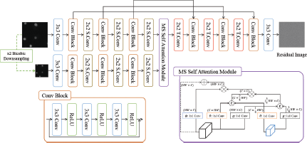
Multi-scale self-attention network for fluorescence image denoising. 2 × 2 S. Conv and 2 × 2 T.Conv denote a stride convolution and transposed convolution with a 2 × 2 convolution filter, respectively.
Multi-scale self-attention network for fluorescence image denoising. 2 × 2 S. Conv and 2 × 2 T.Conv denote a stride convolution and transposed convolution with a 2 × 2 convolution filter, respectively.
3.1 Feature Extractor
The feature extractor comprises a convolution layer, three convolution blocks, and three stride convolutions for downsampling. The first convolution layer has 64 filters, each of which has a size of 3 × 3 × 1 to receive an input grayscale image. Each convolution block comprises three convolution layers, each of which is followed by a rectified linear unit (ReLU) activation function for non-linearity. The convolution layer at the i-th block has 64 × i filters, each of which has a size of 3 × 3 × (64 × i). We add skip connections at three convolution layer intervals to ensure smooth transmission of information. These skip connections also facilitate efficient information propagation between different levels; consequently, the network can be trained with a high efficiency. After passing the convolutional block, a 2 × 2 strided convolution layer is applied for downsampling of the input feature map. We use reflection padding for all the convolution layers to set the spatial sizes of the feature maps which are the same as those of the input image.
3.2 Multi-scale Self-Attention Module
In this subsection, we demonstrate the proposed multi-scale self-attention module. First, we introduce a self-attention module called a non-local block, which was proposed by Wang et al. [48]. Next, we describe a light-weight self-attention module and compare it with the non-local block. Finally, we explicate the proposed multi-scale self-attention module and highlight the advantages of our proposed module in terms of image denoising.
A Non-local Block
Figure 2a shows a non-local block proposed by Wang et al. [48], which is inspired by a non-local means filter [5]. Specifically, the non-local operator is defined as
where x and y are the input and output feature maps, respectively, i and j are the spatial indices of features, xi and xj are the i-th and j-th features of the feature map x, respectively, N is the spatial location of the input image’s feature map, ɡ(xj) is a trainable transform of xj corresponding to a 1 × 1 convolution, w(i, j) is a similarity measure between xi and xj, and +xi indicates a residual connection so that the first term on the right-hand side learns only the residual. With regard to w(i, j), Liu et al. tested various similarity measures such as embedded dot product, symmetric embedded Gaussian, and embedded Gaussian [27]. Herein, we adopted the embedded dot product in w for the light-weight self-attention and multi-scale self-attention modules, which will be described later. Specifically, w(i, j) is defined as
where θ and ϕ are trainable transforms, which are implemented in the non-local block using 1 × 1 convolution.
This non-local block has shown good performance in various fields such as image denoising and super-resolution [27], but there are clear disadvantages in image restoration. In most deep learning networks for image restoration, downsampling operations do not exist. Subsequently, when the feature maps pass via the non-local block, a tremendous amount of calculations involving matrix multiplication is required [57]. The computation cost of matrix multiplication is 2 × HW × HW × C, and as the size increases, the cost increases exponentially. This is very unsuitable for image restoration, and thus, the NLRN [27] reconstructs and attaches very small images using this non-local block during inference.
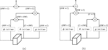
(a) An illustration of a non-local block with embedding Gaussian proposed in [48]. (b) Illustration of a light-weight self-attention module.
(a) An illustration of a non-local block with embedding Gaussian proposed in [48]. (b) Illustration of a light-weight self-attention module.
3.2.1 Light-Weight Self-attention Module
To reduce the computational cost of matrix multiplication in the non-local block, a light-weight self-attention module that can change the order of matrix multiplication is proposed. The structure of the light-weight self-attention module is depicted in Figure 2. As matrix multiplication follows an associative law, a non-local block and a light-weight self-attention module produce the same output. The computational cost of the matrix multiplication in the light-weight self-attention module is 2 × HW × C × C. When H and W are 256, and the number of channels, C, is 256, the computational cost of the light-weight self-attention module is 2 × 2564, but that of a non-local block is 2 × 2565. The computational cost of a light-weight self-attention module is 256 times less than that of a non-local block. Therefore, the light-weight self-attention module is suitable for use in a deep learning network for image restoration.
3.2.2 Multi-scale Self-attention Module
Based on the light-weight self-attention module, we propose a multi-scale self-attention module to fully exploit self-similarity at different scale as shown in Figure 3. The underlying concept behind the proposed multi-scale self-attention module is the exploitation of similar and useful features that may exist at different scales. The multi-scale approach can be especially effective in image denoising, because a downsampled image is less affected by noise. Accordingly, we designed a new extractor for features at different scales to further develop our multi-scale self-attention module. Thus, our module can identify similar non-local features at different scales and merge them together to generate a single output feature. This module receives two features from the input and down-sampled input images. The latter was used herein because the down-sampling operation reduces noise and increases the information available on clearer images. Based on equation 1, the equation of the multi-scale self-attention module is as follows:
where x and y are the input and output feature maps, respectively; x is an input feature map from the downsampled input image; i and j are spatial indices of features; xi and xj are the i-th and j-th features, respectively, of feature map is the j-th feature of ; N and M are the spatial locations of input feature maps from the input image and down-sampled input image, respectively; ɡ(xj ) is a trainable transform of xj, corresponding to a 1 × 1 convolution; wN(i, j) is a similarity measure between xi and xj ; and wM (i, j) is a similarity measure between xi and . The equations of wN(i, j)wM(i, j) are follows:
Then, we substituted equation 4 into equation 3 as below:
where K is the channel location of the feature maps, and c is the channel-wise indices of the features. xc and xc are the c-th spatial information of the feature map x and , respectively. Equation 5 shows that the sequence of calculations does not change the similarity result at multi-scales when measuring self-similarity. Subsequently, we devised a multi-scale self-attention module as shown in Figure 3.
In terms of the computational cost, compared with the two modules introduced earlier, the proposed module has a computational cost of 2.25 × HW × C × C, which is 12.5% more than that of a light-weight self-attention module but significantly lower than that of a non-local block. When H and W are 256, and the number of channels, C, is 256, the multi-scale self-attention module is 228 times lighter than a non-local block. Therefore, the computational cost can be reduced by using the multi-scale self-attention module with the light-weight self-attention module.
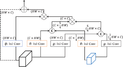
Illustration of the proposed multi-scale self-attention module.
Illustration of the proposed multi-scale self-attention module.
3.3 Decoder
The decoder, which was designed to be symmetrical with the feature extractor structure without stride convolution, consists of one convolution layer, three transposed convolutions for upsampling, and three convolution blocks with the same structure as that used in feature extraction (see Figure 1). After passing each convolutional block via the decoder, a 2 × 2 transposed convolution layer is used to match the spatial resolution of the input image with the downsampled feature map. The final convolution layer has one filter of size 3 × 3 × 64 to transform the feature map into a residual image. The residual image is then subtracted from the input to obtain the final restored image.
3.4 Loss Function
To train our network, we minimized the L1 loss function. Specifically, given a training dataset D = {… (I(i), J(i)…} where I(i) and J(i) are the i-th input noisy image and its corresponding ground truth, respectively, we minimized the following loss function:
where Θ denotes a set of network parameters, and f (I(i);Θ) is a residual image predicted by our network using the parameters Θ.
4 Experiments
4.1 Dataset
To evaluate our network against state-of-the-art techniques, we employed the Fluorescence Microscopy Denoising (FMD) dataset delineated by Zhang et al. [54] and the Widefield Microscopy (W2S) dataset expounded by Zhou et al. [56]. Collaborating with Seoul National University Hospital, we also constructed an ultrasound dataset for bladder volume detection spanning 2022 to 2023.
The FMD dataset encompasses 12,000 authentic confocal, two-photon, and wide-field microscopy images, procured through fluorescence imaging of Bovine Pulmonary Artery Endothelial (BPAE) cells, fixed zebrafish embryos, and preserved mouse brain tissues. By averaging diverse image quantities (S = 2, 4, 8, and 16), we derived four distinct noise levels alongside the raw images. The canonical truth was subsequently ascertained by averaging 50 corresponding noisy fluorescence images. Of the 60,000 image duos, 57,000 were allocated for training and 3,000 for testing, with the data statistics manifesting Poisson-Gaussian noise. Although the inception image dimensions of the training set stood at 512 × 512, they were truncated to 256 × 256 sans overlap for both training and testing.
Conversely, the W2S dataset incorporates noisy wide-field microscopy snapshots of genuine human cells, spanning 120 diverse Fields of View (FOV), with a set of 400 images per FOV. These images correspond to three channels with 488, 561, and 640 nm wavelengths. The dataset demarcated 240 FOVs for training and the remaining 120 for testing. The canonical truth for each FOV was deduced from the mean of 400 images. Like the FMD, this dataset integrated varying noise level images by averaging sets of 2, 4, 8, and 16 wide-field microscopy images. Every image in the W2S dataset adhered to dimensions of 512 × 512 pixels, with statistics also depicting Poisson-Gaussian noise.
Additionally, we procured 10,000 bladder visuals from 100 patients via a 2D ultrasound apparatus. The ground truth was meticulously constructed employing signal processing techniques such as frequency-compounding and wavelet transformation, orchestrated by the device manufacturer. Initially measuring 616 × 660 post-B-mode transformation, these images were resized to 512 × 512.
4.2 Experimental Settings
To train our network, we used 1e−4 as the initial learning rate and decayed it by using a one-cycle scheduler. We used the Adam optimizer [21] with parameters β1 = 0.9, β2 = 0.999, and e = 108. The mini-batch size was 16, and the models were trained for 200 epochs on an Intel Zeon E5-2620 @ 2.0
GHz system and an NVIDIA TITAN RTX (24GB). PyTorch [34] was used to implement and train all the networks.
After evaluating the MSAN with the fluorescence dataset, MSAN and the state-of-the-art methods were applied to denoise fast 3D confocal fluorescence images of 15 μπι microbeads. Fast 3D confocal images were acquired with the following acquisition parameters: a frame rate of 50 ms, a z-step size of 1 μm, the number of 3D confocal fluorescence image stack of 60, and a pixel dwelling time of 15.5 ns. We acquired 50 3D confocal images at the same scene. Among them, the first image was used as the noise image, and the image obtained by averaging 50 images was used as the ground-truth. Each confocal image was denoised using MSAN and other state-of-the-art methods, and a 3D image was then constructed with the denoised images.
4.3 Comparison of Self-Attention Modules
We compared the performance of our proposed multi-scale self-attention module with that of a low-weight self-attention module in fluorescence image denoising in terms of the peak signal-to-noise ratio (PSNR) (dB). As a non-local block proposed by Wang et al. [48] requires approximately 1000 times more memory than the light-weight and multi-scale self-attention modules when trained using the fluorescence microscopy denoising (FMD) dataset, the non-local block was excluded from this comparison.
Comparison of different self-attention modules in terms of PSNR (dB) on an FMD dataset with raw images.
| None attention | Single-scale attention |
| 35.48 | 35.64 |
| Two-scale attention | Three-scale attention |
| 35.78 | 35.72 |
Table 1 compares the PSNRs of different-scale self-attention modules in fluorescence image denoising. We conducted experiments on attention modules at three different scales. Specifically, we used the original and 2 × downsam-pled images on the two-scale attention module, and 4× downsampled images on the three-scale attention module. The two- and three-scale self-attention modules yielded PSNRs of 35.78 and 35.72 dB, respectively, whereas the single-scale self-attention module (which is equivalent to a low-weight self-attention module) yielded a PSNR of 35.64 dB. These results demonstrate that the multi-scale self-attention module is superior to the low-weight self-attention module for fluorescence image denoising in terms of PSNR. For the three-scale self-attention module, we used 4× downsampled images, which not only contain less noise but also result in significant information loss; thus, performance was slightly lower than with the two-scale self-attention module. Consequently, we used a two-scale self-attention module for MSAN. Furthermore, we examined our model’s performance without an attention module, which yielded a PSNR of 35.48 dB. Thus, we confirmed that the multi-scale self-attention module enables high-performance improvements in fluorescence image denoising.
Comparison of interpolation methods in MSAN in terms of PSNR (dB) on an FMD dataset with raw images.
| Nearest neighbor interpolate | Bilinear interpolate | Bicubic interpolate |
|---|---|---|
| 35.71 | 35.65 | 35.78 |
We examined the suitability of interpolation methods for MSAN. As shown in Table 2, the MSAN improved performance when incorporating bicubic interpolation into its framework, compared to alternative methods. Therefore, we adopted bicubic interpolation. In addition, we performed a comparison between the L1 and L2 loss functions in order to identify the most suitable loss function. The L1 loss achieved a PSNR of 0.12 dB higher than the L2 loss and provided sharper images.
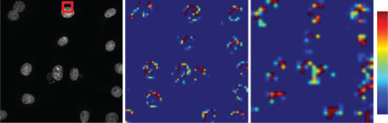
Examples of attention maps from a multi-scale self-attention module for fluorescence image denoising. The middle and right images denote the correlation attention maps of the regions indicated by the red solid rectangle in the left image. Left: fluorescence image; Middle: attention map from an original image; Right: attention map from a downsampled image.
Examples of attention maps from a multi-scale self-attention module for fluorescence image denoising. The middle and right images denote the correlation attention maps of the regions indicated by the red solid rectangle in the left image. Left: fluorescence image; Middle: attention map from an original image; Right: attention map from a downsampled image.
We also investigated the advantages of a multi-scale self-attention module in fluorescence image denoising. To further analyze this module, the attention maps for non-local operations are shown in Figure 4. The middle and right images show the attention maps from the original and downsam-pled images, respectively. The multi-scale self-attention module exploits self-similarity at different scales to enhance the performance of fluorescence image denoising.
| Methods | PSNR(dB)/SSIM | ||||||
|---|---|---|---|---|---|---|---|
| The number of raw images for averaging | Average value | ||||||
| 1 | 2 | 4 | 8 | 16 | |||
| Traditional method | Noised | 27.22 / 0.5442 | 30.08 / 0.6800 | 32.86 / 0.7981 | 36.03 / 0.8892 | 39.70 / 0.9487 | 33.18 / 0.7740 |
| NLM | 31.25 / 0.7503 | 32.85 / 0.8116 | 34.92 / 0.8763 | 37.09 / 0.9208 | 40.04 / 0.9540 | 35.23 / 0.8626 | |
| BM3D | 32.71 / 0.7922 | 34.09 / 0.8430 | 36.05 / 0.8970 | 38.01 / 0.9336 | 40.61 / 0.9598 | 36.29 / 0.8851 | |
| KSVD | 32.02 / 0.7746 | 33.69 / 0.8327 | 35.84 / 0.8933 | 37.79 / 0.9314 | 40.36 / 0.9585 | 35.94 / 0.8781 | |
| EPLL | 32.61 / 0.7876 | 34.07 / 0.8414 | 36.08 / 0.8970 | 38.12 / 0.9349 | 40.83 / 0.9618 | 36.34 / 0.8845 | |
| WNNM | 32.52 / 0.7880 | 34.04 / 0.8419 | 36.04 / 0.8973 | 37.95 / 0.9334 | 40.45 / 0.9587 | 36.20 / 0.8839 | |
| PURE-LET | 31.95 / 0.7664 | 33.49 / 0.8270 | 35.29 / 0.8814 | 37.25 / 0.9212 | 39.59 / 0.9450 | 35.51 / 0.8682 | |
| Early DL | DnCNN* | 34.88 / 0.9063 | 36.02 / 0.9257 | 37.57 / 0.9460 | 39.28 / 0.9588 | 41.57 / 0.9721 | 37.86 / 0.9418 |
| IRCNN* | 34.70 / 0.8977 | 35.83 / 0.9217 | 37.37 / 0.9439 | 39.10 / 0.9571 | 41.18 / 0.9695 | 37.64 / 0.9380 | |
| MemNet* | 33.04 / 0.8314 | 35.23 / 0.9018 | 37.16 / 0.9383 | 39.02 / 0.9555 | 41.15 / 0.9687 | 37.12 / 0.9191 | |
| SotA DL | Noise2Noise* | 35.40 / 0.9187 | 36.40 / 0.9230 | 37.59 / 0.9481 | 39.43 / 0.9601 | 41.45 / 0.9724 | 38.05 / 0.9445 |
| MWCNN* | 35.40 / 0.9190 | 36.33 / 0.9329 | 37.62 / 0.9489 | 39.32 / 0.9608 | 41.39 / 0.9736 | 38.01 / 0.9470 | |
| RIDNet* | 35.63 / 0.9167 | 36.41 / 0.9325 | 37.97 / 0.9498 | 39.55 / 0.9610 | 41.58 / 0.9740 | 38.23 / 0.9468 | |
| DPDN* | 35.64 / 0.9189 | 36.35 / 0.9322 | 38.02 / 0.9501 | 39.51 / 0.9611 | 41.50 / 0.9744 | 38.20 / 0.9472 | |
| WF-UNet* | 34.45 / 0.8978 | 35.58 / 0.9204 | 37.29 / 0.9427 | 38.97 / 0.9561 | 41.23 / 0.9689 | 37.50 / 0.9372 | |
| MSAN* (Ours) | 35.78 / 0.9216 | 36.85 / 0.9362 | 38.19 / 0.9507 | 39.70 / 0.9621 | 41.31 / 0.9738 | 38.37 / 0.9489 | |
4.4 Performance Evaluation of MSAN in Fluorescence Image Denoising
The MSAN performance was compared with that of other state-of-the-art denoising methods, including a non-local means filter (NLM) [5], BM3D [9], KSVD [1], EPLL [58], WNNM [17], PURE-LET [30], IRCNN [53], DnCNN [52], MemNet [44], Noise2Noise [23], MWCNN [29], WF-UNet [36], RIDNet [2] and DPDN [19]. We used the PSNR (dB) and structural similarity index (SSIM) [49] as evaluation metrics. These two metrics are widely used to evaluate denoising methods. Higher PSNR and SSIM values indicate that the denoised image is more similar to its ground truth. For the classical denoising approaches including NLM, BM3D, KSVD, EPLL, and WNNM, the Poisson-Gaussian noise was transformed into Gaussian noise using a nonlinear variance-stabilizing transformation (VST) [31], following which the noise level was estimated using [14]. In contrast, for the deep learning-based approaches including DnCNN, MemNet, Noise2Noise (N2N), MWCNN, WF-UNet, and DPDN, each network was trained with the same training strategy as MSAN, as mentioned in Section 3.4.
Table 3 presents the denoising results of MSAN and other state-of-art models on the FMD dataset. Our proposed MSAN outperforms the other methods at all noise levels except when the number of images required for averaging was 16. Classical denoising approaches via a non-blind strategy showed lower performance than the deep learning-based approaches when using a blind strategy in denoising the fluorescence images. In classical denoising approaches, EPLL and BM3D showed higher performance than other classical methods. Compared to EPLL, N2N, MWCNN, RIDNet, DPDN, and out method showed a notable PSNR gain of 1.71 dB, 1.67 dB, 1.86 dB, and 1.89 dB, respectively. In contrast, MSAN exhibited a 2.03 dB higher PSNR than EPLL.In addition, MSAN achieved a significantly higher mean PSNR (38.366 dB) than MWCNN (38.012 dB), N2N (38.054 dB), RIDNet (38.228 dB), and DPDN (38.198 dB). In terms of SSIM, MSAN also showed the highest performance at all noise levels. The mean SSIM of the MSAN was 0.94888 while that of the MWCNN and DPDN was 0.94704 and 0.94724, respectively. Note that MSAN required less memory and shorter computation time than MWCNN.
| Methods | PSNR(dB)/SSIM | ||||||
|---|---|---|---|---|---|---|---|
| The number of raw images for averaging | Average value | ||||||
| 1 | 2 | 4 | 8 | 16 | |||
| Traditional method | Noised | 21.34 / 0.3612 | 23.78 / 0.4480 | 26.38 / 0.5473 | 29.10 / 0.6537 | 31.92 / 0.7555 | 26.50 / 0.5531 |
| NLM | 23.68 / 0.7731 | 26.61 / 0.8204 | 29.69 / 0.8597 | 32.57 / 0.8899 | 35.29 / 0.9169 | 29.57 / 0.8520 | |
| BM3D | 24.18 / 0.8081 | 27.20 / 0.8508 | 30.33 / 0.8834 | 33.21 / 0.9075 | 36.00 / 0.9298 | 30.18 / 0.8760 | |
| KSVD | 23.83 / 0.7841 | 26.83 / 0.8307 | 29.99 / 0.8696 | 32.93 / 0.8989 | 35.80 / 0.9255 | 29.88 / 0.8617 | |
| EPLL | 24.09 / 0.7998 | 27.12 / 0.8454 | 30.25 / 0.8803 | 33.14 / 0.9059 | 35.94 / 0.9291 | 30.11 / 0.8721 | |
| WNNM | 24.01 / 0.8005 | 27.04 / 0.8450 | 30.20 / 0.8797 | 33.12 / 0.9053 | 35.97 / 0.9288 | 30.07 / 0.8719 | |
| PURE-LET | 24.09 / 0.8000 | 27.16 / 0.8434 | 30.29 / 0.8783 | 33.15 / 0.9026 | 35.89 / 0.9260 | 30.12 / 0.8701 | |
| Early DL | DnCNN* | 33.51 / 0.9029 | 35.04 / 0.9189 | 37.23 / 0.9337 | 38.62 / 0.945 | 40.15 / 0.9540 | 36.91 / 0.9309 |
| IRCNN * | 33.49 / 0.9094 | 34.94 / 0.9235 | 37.08 / 0.9356 | 38.68 / 0.9477 | 39.87 / 0.9557 | 36.81 / 0.9344 | |
| MemNet* | 31.45 / 0.8767 | 34.28 / 0.9121 | 35.76 / 0.9233 | 37.20 / 0.9319 | 39.17 / 0.9493 | 35.57 / 0.9187 | |
| SotA DL | Noise2Noise* | 32.93 / 0.9055 | 35.19 / 0.9203 | 37.02 / 0.9313 | 38.41 / 0.9467 | 40.13 / 0.9556 | 36.74 / 0.9319 |
| MWCNN* | 32.89 / 0.8946 | 34.69 / 0.9179 | 36.90 / 0.9337 | 38.31 / 0.9447 | 40.00 / 0.9547 | 36.56 / 0.9291 | |
| RIDNet* | 33.70 / 0.8707 | 34.91 / 0.8983 | 36.97 / 0.9254 | 38.53 / 0.9446 | 40.20 / 0.9589 | 36.86 / 0.9196 | |
| DPDN* | 33.51 / 0.8728 | 35.33 / 0.8915 | 37.07 / 0.9231 | 38.54 / 0.9456 | 39.81 / 0.9501 | 36.85 / 0.9166 | |
| WF-UNet* | 32.67 / 0.7366 | 34.31 / 0.8316 | 35.88 / 0.8507 | 37.04 / 0.8714 | 39.26 / 0.8895 | 35.83 / 0.8360 | |
| MSAN* (Ours) | 33.79 / 0.9102 | 35.57 / 0.9267 | 37.33 / 0.9378 | 38.81 / 0.9488 | 40.20 / 0.9538 | 37.14 / 0.9354 | |
Table 4 presents a quantitative comparison with the W2S dataset. Compared with results for the FMD dataset, our MSAN exhibited the highest performance, except for the case of 16 averaged images. For this dataset, our method yielded a PSNR 0.23 dB higher than the second highest DnCNN. These results therefore confirm that the MSAN outperforms other state-of-the-art methods in fluorescence image denoising in a more efficient manner. Furthermore, the performance of MSAN was compared to that of other state-of-the-art methods in denoising wide-field, confocal, and two-photon fluorescence images of different biological samples in Figure 5 and Table 5.
Quantitative comparisons between MSAN and other methods in terms of PSNR and SSIM with the proposed our 3D confocal fluorescence imaging dataset. The first and second best performances are denoted in red and blue, respectively.
| Methods | Noisy | NLM | BM3D | KSVD | EPLL | WNNM | PURE-LET | DnCNN |
|---|---|---|---|---|---|---|---|---|
| PSNR | 37.79 | 45.92 | 47.13 | 44.56 | 44.82 | 44.50 | 38.69 | 46.77 |
| SSIM | 0.8728 | 0.9803 | 0.9831 | 0.9740 | 0.9742 | 0.9715 | 0.8874 | 0.9822 |
| Methods | IRCNN | MemNet | Noise2Noise | MWCNN | WF-UNet | RIDNet | DPDN | MSAN |
| PSNR | 46.61 | 44.97 | 47.13 | 45.44 | 47.09 | 46.14 | 45.74 | 47.36 |
| SSIM | 0.9788 | 0.9688 | 0.9821 | 0.9733 | 0.9836 | 0.9772 | 0.9741 | 0.9850 |
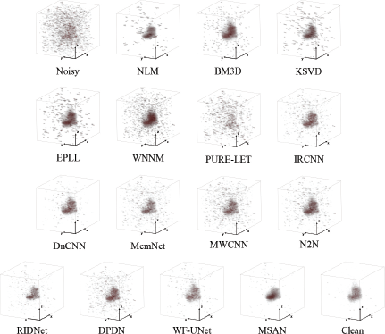
Qualitative comparisons of MSAN and other state-of-the-art methods with 3D confocal fluorescence image dataset.
Qualitative comparisons of MSAN and other state-of-the-art methods with 3D confocal fluorescence image dataset.
Figure 6 shows the qualitative comparisons between the MSAN and other state-of-the-art methods on the FMD dataset. It can be seen that the MSAN offers clearer images with less noise compared to the other methods. In the first image, which is the confocal fluorescence image of a fixed zebrafish embryo, our method preserves more details in the denoised image compared to the other methods. The second and third images, which are the two-photon fluorescence images and the wide-field fluorescence images of BPAE cells, respectively, demonstrated that our method achieves the least artistic denoised images compared to the other methods. Figure 7 shows a qualitative comparison of the W2S dataset. The regions indicated by the red and yellow solid rectangles are magnified. As shown in Figure 7, MSAN preserved the most information and details out of all the methods tested. Although the images obtained by WF-UNet are sharper than those of other existing models, they are less clean than those obtained by MSAN. It should be noted here that MSAN yields a 0.50 dB higher PSNR and 0.1998 higher SSIM than WF-UNet.
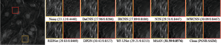
Qualitative comparison on the FMD dataset [54]. Left: Ground-truth images. Right: Magnified views of different image denoising results. The first image shows a confocal fluorescence image of fixed zebrafish embryos. The second one shows a two-photon fluorescence image of BPAE cells. The third shows a wild-field fluorescence of BPAE cells.
Qualitative comparison on the FMD dataset [54]. Left: Ground-truth images. Right: Magnified views of different image denoising results. The first image shows a confocal fluorescence image of fixed zebrafish embryos. The second one shows a two-photon fluorescence image of BPAE cells. The third shows a wild-field fluorescence of BPAE cells.
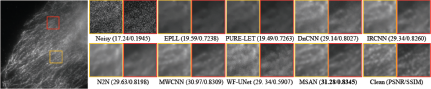
Qualitative comparison on the W2S dataset [56]. Left: Ground-truth images. Right: Magnified views of different image denoising results. The first and second images are conventional wide-field fluorescence images of human cells.
Qualitative comparison on the W2S dataset [56]. Left: Ground-truth images. Right: Magnified views of different image denoising results. The first and second images are conventional wide-field fluorescence images of human cells.
Finally, to further ensure the superiority of MSAN compared to other state-of-the-art methods, MSAN and other methods were applied to denoise 3D confocal fluorescence images of microbeads. For this comparison, we used the MSAN and other methods trained in the FMD dataset. In this comparison, MSAN achieved the highest PSNR (47.36 dB) and SSIM (0.9850) in the fluorescence image denoising (Table 5) as well as the clearest 3D confocal fluorescence image compared to the other methods (Figure 5).
4.5 Performance Evaluation of MSAN in Ultrasound Image Denoising
In our quantitative analysis presented in Table 6, we found that MSAN consistently outperforms various other state-of-the-art models on the ultrasound image dataset. Specifically, MSAN achieved an average PSNR value of 30.98 dB, which is notably higher than the second-best model, DPDN, at 29.21 dB, and far superior to classical methods such as BM3D and EPLL, which registered PSNR values of 25.82 dB and 25.60 dB, respectively. Similarly, the mean SSIM score for MSAN was 0.8233, substantially outperforming other competing algorithms like MWCNN and DPDN, which achieved SSIM scores of 0.7752 and 0.7926 respectively. Moreover, the computational efficiency of the MSAN’ is evident; it required less memory and demonstrated faster computation times than other models like MWCNN.
Quantitative comparisons between MSAN and other methods in terms of PSNR and SSIM with the proposed 2D ultrasound imaging dataset. The first and second best performances are denoted in red and blue, respectively.
| PSNR(dB)/SSIM | |||||||
|---|---|---|---|---|---|---|---|
| Methods | The number of raw images for averaging | Average value | |||||
| 1 | 2 | 4 | 8 | 16 | |||
| Traditional method | Noised | 20.67 / 0.2980 | 21.00 / 0.3917 | 23.00 / 0.4770 | 23.67 / 0.5559 | 23.75 / 0.6610 | 22.42 / 0.4767 |
| NLM | 21.22 / 0.6428 | 23.03 / 0.7179 | 25.99 / 0.7328 | 27.88 / 0.7448 | 29.32 / 0.7985 | 25.49 / 0.7274 | |
| BM3D | 21.38 / 0.6941 | 24.47 / 0.7147 | 26.06 / 0.7499 | 28.43 / 0.7774 | 28.78 / 0.8093 | 25.82 / 0.7491 | |
| KSVD | 21.50 / 0.6635 | 24.02 / 0.6971 | 24.94 / 0.7588 | 26.90 / 0.7898 | 30.15 / 0.7898 | 25.50 / 0.7398 | |
| EPLL | 21.31 / 0.6852 | 23.76 / 0.7317 | 25.31 / 0.7467 | 27.79 / 0.7759 | 29.83 / 0.8138 | 25.60 / 0.7507 | |
| WNNM | 22.19 / 0.6718 | 23.55 / 0.7293 | 25.23 / 0.7468 | 27.27 / 0.7560 | 29.67 / 0.7634 | 25.58 / 0.7335 | |
| PURE-LET | 22.42 / 0.6783 | 23.20 / 0.7344 | 25.95 / 0.7775 | 28.30 / 0.7511 | 29.54 / 0.7863 | 25.88 / 0.7455 | |
| Early DL | DnCNN | 26.08 / 0.7499 | 27.89 / 0.7632 | 29.36 / 0.8021 | 30.67 / 0.7843 | 30.89 / 0.8444 | 28.98 / 0.7888 |
| IRCNN | 25.86 / 0.7688 | 28.07 / 0.7883 | 28.60 / 0.7900 | 30.63 / 0.8349 | 30.74 / 0.8080 | 28.78 / 0.8000 | |
| MemNet | 25.23 / 0.7389 | 26.89 / 0.8134 | 28.33 / 0.7930 | 30.17 / 0.7802 | 31.77 / 0.8287 | 28.48 / 0.7948 | |
| SotA DL | Noise2Noise | 26.80 / 0.7541 | 27.48 / 0.7748 | 29.16 / 0.7748 | 29.90 / 0.7799 | 32.35 / 0.8017 | 29.14 / 0.7771 |
| MWCNN | 26.34 / 0.7448 | 27.48 / 0.7815 | 28.75 / 0.7654 | 30.61 / 0.8049 | 30.62 / 0.7794 | 28.76 / 0.7752 | |
| RIDNet | 25.86 / 0.7263 | 26.79 / 0.7908 | 28.90 / 0.7932 | 30.74 / 0.7909 | 30.73 / 0.8079 | 28.60 / 0.7818 | |
| DPDN | 26.87 / 0.7340 | 27.01 / 0.7608 | 28.96 / 0.8279 | 31.10 / 0.8155 | 32.11 / 0.8247 | 29.21 / 0.7926 | |
| WF-UNet | 25.40 / 0.6283 | 27.98 / 0.7034 | 29.26 / 0.7306 | 29.80 / 0.7487 | 30.22 / 0.7394 | 28.53 / 0.7101 | |
| MSAN (Ours) | 27.88 / 0.7820 | 30.24 / 0.8290 | 30.80 / 0.8338 | 32.76 / 0.8408 | 33.25 / 0.8330 | 30.98 / 0.8233 | |
Additionally, it is worth noting that MSAN’s high performance was consistent across different numbers of raw images used for averaging. Even when the number of averaged images was as low as one, MSAN stood out with a PSNR of 26.85 dB and an SSIM of 0.8654, setting a new benchmark for ultrasound image denoising. The only exception to top-ranking performance occurred when the number of averaged images was 16; however, even in this scenario, MSAN was highly competitive. The experimental results showcase MSAN’s robustness and adaptability to different imaging conditions, a crucial factor often overlooked in evaluating denoising algorithms. With its computational efficiency and high-quality denoising, MSAN demonstrates a well-rounded superiority pivotal for real-world medical imaging applications.
Further visual validation is provided in Figure 8, where qualitative comparisons clearly show the capacity of the MSAN model for preserving essential details while minimizing noise. Particularly in intricate regions of the ultrasound images, denoted by the red and yellow rectangles, MSAN’s superior performance becomes abundantly clear. These quantitative and qualitative results jointly establish the capability of our model to effectively denoise ultrasound images, surpassing both classical and state-of-the-art deep-learning algorithms.
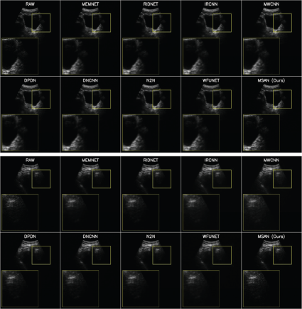
Qualitative comparisons of MSAN and other state-of-the-art methods with 2D ultrasound image dataset.
Qualitative comparisons of MSAN and other state-of-the-art methods with 2D ultrasound image dataset.
In summary, in the context of bladder ultrasound imaging, the advantages offered by MSAN go beyond traditional metrics like PSNR and SSIM. Accurate bladder imaging is vital for various medical applications, including monitoring urinary retention, postoperative care, and oncological assessments. MSAN’s ability to effectively denoise while preserving crucial anatomical structures can significantly enhance diagnostic precision, thereby aiding in the early detection and treatment of bladder-related conditions. Even minor noise or artifacts can lead to misinterpretations, so the model’s superior denoising capabilities are particularly impactful. Furthermore, the computational efficiency of MSAN makes it well-suited for integration into real-time imaging systems. Overall, MSAN represents a methodological advancement in image denoising and a significant contribution to the broader field of bladder healthcare.
5 Discussion and Conclusions
We introduced a multiscale attention network designed for denoising tasks in both fluorescence microscopy and ultrasound imaging. The performance of our network was compared against that of other state-of-the-art methods on both ultrasound and fluorescence microscopy images. The experimental results revealed that our network outperformed other state-of-the-art denoising methods in terms of PSNR and SSIM. Our network yielded the most noteworthy SSIM scores of 0.9216, 0.9362, 0.9507, 0.9621, and 0.9738. These values surpassed those of other methods by a margin ranging from 0.002 to 0.086 across varying noise levels (with averaging image counts of 1, 2, 4, 8, and 16). Furthermore, our network achieved PSNR values that surpassed those achieved by MWCNN and N2N by 1.92 dB and 0.23 dB, respectively, within our 3D confocal fluorescence image denoising dataset.
Our MSAN represents a cutting-edge, multi-scale, self-similarity-based deep learning methodology tailored for denoising ultrasound and fluorescence images. In the proposed MSAN, we have incorporated additional convolution layers by lightening the self-attention module to extract multi-scale features from the training dataset. In addition, building upon the notion that valuable features with similarities may exist across various scales, we proposed a multi-scale self-attention module. This module capitalizes on self-similarity at multiple scales, and our ablation study confirms its superiority over the single-scale counterpart. As discussed in Section 3.2, the multi-scale self-attention module exhibits a weight reduction of approximately 200 times when compared with the nonlocal block employed in NLRN [27]. NLRN, being the pioneer in integrating self-similarity into deep neural networks for image restoration, demands a substantial memory overhead. This poses challenges for training the network due to the spatial dimensions of the FMD training data, set at 256 × 256.
Recently, numerous deep learning networks have emerged to enhance image denoising performance across diverse domains. These proposed methodologies encompass a spectrum of techniques, spanning from the integration of stacked convolutional layers to the utilization of dedicated subnetworks for noise intensity assessment. Among these advancements is the blind universal image fusion denoiser. The blind universal image fusion denoiser [12] comprises a pair of networks, with one dedicated to estimating noise intensity. Despite its outstanding performance in synthetic blind image denoising tasks, the applicability of this method to real-world images poses challenges. Approaches for joint image denoising and super-resolution have also been proposed. It has been demonstrated that a deep residual channel attention network (RCAN) [55] effectively improves the quality of four-dimensional fluorescence microscopy data [6]. However, as RCAN primarily focuses on super-resolution, it results in discrepancies between the spatial resolutions of input and output images. Consequently, this approach is not suitable for our specific task.
Furthermore, this work represents an endeavor that enhances performance by harnessing multi-scale self-similarity within the realm of image restoration. It also applies the concept that beneficial features can manifest at diverse scales, as evidenced by the attention map. Our findings indicate significant promise for the proposed MSAN in denoising a variety of fluorescence images, including wide-field, confocal, and two-photon, as well as ultrasound images. Moreover, the versatility of the multi-scale self-attention module extends to other image restoration tasks, including super-resolution, deblurring, and deblocking. These areas remain a focus for our future research endeavors. In response to the importance of testing the robustness and versatility of our method, it is strongly significant to conduct comprehensive cross-dataset experiments. The remaining future work will explore how well the MSAN method adapts and performs when faced with data from varied sources, different domains, and diverse conditions.
This work was supported by the Korea Medical Device Development Fund grant funded by the Korea government (the Ministry of Science and ICT, the Ministry of Trade, Industry and Energy, the Ministry of Health & Welfare, the Ministry of Food and Drug Safety, 1711179383, RS-2022-00141185).

