


Versatile Video Coding (VVC) is a modern video compression standard designed to efficiently encode high definition video content, regardless of its diversity. It is expected to deliver superior compression performance compared to the previous standard, High Efficiency Video Coding (HEVC). However, the bit rate control problem for VVC can still be improved. To address this issue, a learning-based initial frame Quantization Parameter (QP) prediction algorithm has been proposed in this paper. This algorithm extracts information from image pixels and maps it to a feature matrix to reduce its additional cost. Furthermore, the problem of inaccurate determination of VVC QPs has been addressed by building a residual network to represent the frame complexity progressively and learning the optimal relationship between QPs and the target bit rate. Experimental results show that the proposed method reduces the control error from 10.74% to 7.19% compared to the original encoder.
1 Introduction
Recently, the rapid advancement of 8K resolution, High Dynamic Range (HDR) imagery, and Virtual Reality (VR) technology has necessitated urgent improvements in video compression performance [28]. The latest video coding standard, Versatile Video Coding (VVC) [3], aims to halve the bit rate compared to its predecessor, High Efficiency Video Coding (HEVC) [25], while maintaining the same video quality through the introduction of innovative technologies. Despite significant advancements in VVC’s performance, Rate Control (RC) remains a critical aspect that urgently requires optimization for market introduction [18].
RC technology is designed to ensure minimum distortion while operating under a constraint bit rate. In the case of VVC, the RC module follows the same method used in HEVC, which involves the R-(A) model for estimating the Quantization Parameter (QP). However, VVC introduces many new technologies that improve the accuracy of intra-frame and inter-frame predictions, which further strengthens the dependency between data [30]. As a result, existing RC research may not fully address VVC’s encoding characteristics. Therefore, studying adaptive RC techniques that align with VVC’s new features is crucial to enhancing VVC’s encoding performance.
Nowadays, research on RC optimization in video coding is primarily focused on optimizing the Rate-Distortion (R-D) model [5,7,12,14,19,20,27,33] and predicting key parameters [2,4,8,9,10,11,13,15,16,17,22,23,29,31,32]. The optimization algorithms grounded in the R-D model prioritize the prediction of bit rates for encoded frames or Coding Tree Units (CTUs) by constructing sophisticated mathematical models. These models aim to capture the intricate relationships between video content, encoding settings, and the target bit rates, enabling more precise control over the coding process. In contrast, RC algorithms that leverage predictive parameters concentrate on efficiently managing bit rates or QPs through a combination of advanced training techniques and dynamic resource allocation strategies. By analyzing historical data and incorporating machine learning algorithms, these approaches aim to optimize the encoding process by accurately predicting the optimal QPs for each frame or CTUs, given its unique characteristics and the overall coding goals. Notably, within the realm of parameter-based rate control algorithms, accurate prediction of QPs for initial frames or I-frames holds particular significance. These frames serve as references for subsequent encoded frames, meaning that any inaccuracies in their quantization can propagate throughout the video sequence, negatively impacting both encoding performance and rate control precision. Therefore, researchers in this field are actively exploring ways to enhance the predictive accuracy of these algorithms, ensuring that the resulting videos maintain high visual quality while adhering to strict bit rate constraints.
To solve this issue, we propose a learning-based initial frame QP prediction algorithm. The main contributions of this paper are summarized as follows.
We have empirically verified the importance of the initial frame QP through theory and statistical experiments, and the results of the statistical experiments have demonstrated the shortcomings of the current VVC in representing image complexity.
We propose a learning-based initial frame 𝒬P prediction algorithm. The network converts brightness and chromaticity information through preprocessing modules and combines the information with target bits, to achieve a rough to detailed representation of frame content.
We use a multi-𝒬P optimization approach to gather effective raw data based on experimental requirements and fine-tuned the 𝒬P prediction network to enabling precise 𝒬P predictions.
Our proposed algorithm reduces the bit Control Error (CE) and has better R-D performance compared to VTM13.0. The rationality of our designed algorithm was also verified and analyzed through various experiments and analyses.
2 Related Work
2.1 Optimizing the R-D Model
To optimize the R-D model, Li et al. [12] introduced modifications to the R-(λ) model by examining the influence of skip division blocks on R-D parameter estimation and the inter-frame quality dependence. Chen et al. [5] employed a quadratic function to construct an R-D model, achieving improved bit allocation accuracy compared to the hyperbolic model. Liu et al. [19] augmented the traditional code RC problem by incorporating objective functions for minimizing average distortion and quality fluctuations, optimizing the (λ)-domain model. Mao et al. [20] proposed the use of composite Cauchy coefficients to model transformation parameters, demonstrating superior performance compared to the original Gaussian model. Wang et al. [27] extracted video texture features using anisotropic filters and leveraged machine learning techniques to construct R-D models, thereby enhancing the model’s adaptability to different video content. Zhou et al. [33] considered the issue of visual differences in High Dynamic Range (HDR) video and built an R-D model based on this issue. Guo et al. [7] proposed a pre-encoding based temporal dependent R-D optimization that adaptively adjusted QPs and Lagrange multipliers according to the distortion effect factors. Liao et al. [14] considered that the accuracy of the hyperbolic R-D model could be further improved by increasing the order of the R-D model. They proposed high-order R-D models and the corresponding one-pass frame-level RC algorithms for video coding. Zhao et al. [30] employed the deep convolutional network to extract the spatial-temporal neighboring coding features and fuse all reference features to determine an optimal intra coding depth. They also employed a probability-based model and the spatial-temporal coherence to select the candidate partition modes within the optimal coding depth.
2.2 Predicting Key Parameters for RC
For parameter prediction in RC, Brand et al. [2] integrated manually extracted feature information and employed a linear model to precisely estimate the target bit, leading to enhanced bit allocation accuracy. Lin et al. [16] leveraged game theory to determine the optimal (λ), optimizing bit allocation at the CTU level and enhancing the overall R-D performance. Hyun et al. [9] utilized Bayesian recursion to accurately predict target bits, enabling more precise bit allocation for uncoded frames. Raufmehr et al. [22] investigated the relationship between bit consumption, buffer size, and QPs, using the former two to anticipate changes in QPs. Zhou et al. [32] addressed the RC challenge in HEVC using deep reinforcement learning. They trained a deep neural network to predict optimal QPs, aiming to minimize distortion, buffering, and quality fluctuations. Li et al. [10] optimized bit allocation for multiview texture videos based on interview dependency and spatiotemporal correlation. Chen et al. [4] initiated an effective learning-based particle swarm optimization for spatial and temporal coding to determine the optimal parameters at the CTU level.
2.3 Initial Frame QP
During video encoding, the initial frame plays a crucial role as a reference for subsequent frames in inter-frame prediction. The allocation of bits and QP for this frame has a significant impact on the overall quality of the video sequence. In practical application scenarios, due to the lack of additional reference information in the initial frame, the bit allocation and rate distortion model of the initial frame are determined based on prior values. In order to improve the quality of the initial frame, the encoder allocates more bits to the initial frame, which affects encoding efficiency. If the QP is set too high, it can degrade the quality of the initial frame, thereby affecting all subsequent frames. Conversely, a low QP may result in insufficient bits allocated for later frames. To enhance encoding efficiency, researchers have explored content-based bit allocation strategies for the initial frame. Yan and Wang [29] introduced a novel bit rate control model tailored to the image complexity for I-frame bit rate control in AVC/H.264. Li et al. [11] employed a convolutional neural network to predict content-related parameters for bit rate control, enabling a more precise determination of the QP for the initial frame. Huang et al. [8] utilized feature extraction and machine learning techniques to predict the QP of the initial frame in VVC, effectively reducing the CE compared to the original encoder. Ren et al. [23] proposed a QP derivation module that constructs several spatiotemporal characteristics into key-frame QP determination through an efficient pre-analysis progress. An adaptive delta-QP value is generated to address the conflict between the low compression efficiency of intra-only frames and the critical predictive basis of temporal-underlying frames.
3 Proposed Method
3.1 Statistical Analysis of RC
In VTM13.0 [24], the initial frame’s QP is determined through the Sum of Absolute Hadamard Transformed Differences (SATD)-based R-(λ) Model confirmation. To highlight the limitations of the VVC primitive encoder in accurately setting the initial frame’s QP, this section presents an experimental analysis of the VTM’s coding efficiency within its Rate Control (RC) module. This analysis is conducted through two statistical experiments: CE assessment and image complexity representation using SATD.
Employing the BQSquare sequence, we investigate the relationship between CE and the number of encoded frames using fixed QP coding in the All Intra (AI) configuration. Figure 1 reveals that the initial frame lacks prior information, leading to a substantial discrepancy between the allocated and actual encoded bit counts. As encoding progresses, frame-level RC adjusts relevant parameters to mitigate CEs. This underscores the significance of the initial frame’s QP in determining the RC accuracy for the current and subsequent frames.
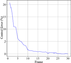
Figure 2 illustrates the distribution of SATD values for the initial frames of the BQSquare sequence. The numbers in the left figure represent the actual encoded bit count, while the numbers in the right figure correspond to the SATD values. Notably, it can be observed that SATD does not offer an accurate representation of image complexity. For instance, there is a significant disparity in the actual bit consumption between the CTU in the first row and first column compared to the CTU in the second row and first column, despite their relatively similar SATD values. Conversely, the difference in actual bit consumption between the CTU in the second row, second column, and the CTU in the second row, third column is minor, yet the SATD values differ significantly. These observations underscore the limitations of SATD as a sole metric for image complexity assessment.
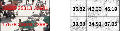
In summary, the initial frame experiences a substantial bit CE due to imited reference information, leading to implications for the bit allocation f subsequent frames. Additionally, SATD fails to adequately represent the lomplexity of images. Under a fixed target bit rate, variations in QP yield istinct encoding outcomes. Identifying the optimal QP is crucial to enhancing he overall R-D performance.
1.2 Initial Frame QP Prediction Network
The residual network depicted in Figure 3 comprises three key components: information preprocessing, target bit fusion, and feature extraction. The preprocessing stage characterizes the image’s complexity through metrics such as standard deviation and gradient. Subsequently, the feature extraction module employs network learning to provide a more nuanced representation of image complexity. To enhance prediction accuracy, the network integrates target bit information at the interface of these two modules. This integration enables the prediction of the initial frame’s QP value based on both image complexity and target bit, thereby optimizing the control performance of the current and subsequent frames.
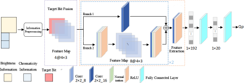
Information Preprocessing: This module is designed to reduce the computational complexity of neural networks and adapt to video sequences of different resolutions. The preprocessing module extracts global and local features of the image for subsequent convolutional neural network prediction. The features are represented using standard deviation and gradients, and the gradients are calculated using the Sobel operator. The specific representation form is as follows:
Global features: Global features represent the complexity of the entire image, represented by the difference between pixels. The larger the difference, the more complex the image is, as shown in Equation (1),
where A represents the pixel matrix.
Local features: Local features represent the local pixel characteristics of an image and the complexity of the entire image is represented by measuring the differences in local pixels. We calculate local features in units of CTU size, with a brightness CTU size of 128 × 128, with a chromaticity CTU size of 64 × 64. The CTU at the boundary is of actual size. As shown in Equation (2).
where F4–6 represents the extreme difference of all N CTUs. F7–9 represents the extreme difference of all R rows. F10–12 represents the extreme difference of all C columns. Bn represents the nth CTU. Bi,j represents the CTU in the i-th row and j-th column. f represents the extraction method, including standard deviation, Sobel horizontal operator, and Sobel vertical operator.
By separately obtaining global and local features for the YUV component, the preprocessing feature matrix shown in Equation (3) can be obtained. This matrix serves as a rough representation of image complexity and will be used for subsequent neural network predictions.
Target Bit Fusion: The determination of QP cannot solely rely on feature information. Additional factors are necessary for accurate prediction. In the R-D model, QP is represented by λ, which is influenced by both the target bit and content parameters. Therefore, the target bit plays a pivotal role in determining the optimal QP. In the designed network model, the target bits are initially expanded into a 1@4x3 matrix, where “4x3” represents the number of rows and columns of the matrix. “1” represents the number of concatenated matrices. “@” represents the concatenation of matrices in dimensions. Subsequently, they are dimensionally concatenated with the input feature maps to create a 4@4x3 information matrix. This enhanced matrix serves as an input to the feature extraction module, facilitating more accurate predictions by the network.
Feature Extraction: This module is designed for the meticulous extraction of texture features, employing a residual skip structure. As depicted in Figure 3, the network module incorporates a dual-branch architecture, which not only facilitates effective feature extraction but also accelerates the network’s convergence speed. In Branch 1, a convolutional block is utilized for feature extraction. Meanwhile, Branch 2 undergoes two convolutional blocks for deeper feature extraction. The feature maps from both branches are then combined in an additive manner. Subsequently, the fused features pass through another convolutional block for further refinement, resulting in the final feature map. For network output, the feature map is flattened into a one-dimensional vector and connected to a fully connected layer. Specifically, the initial fully connected layer comprises 20 neurons, while the second layer, serving as the regression output layer, contains a single neuron.
3.3 Multi QP Optimization Strategy
The multi QP strategy determines the optimal QPs through an exhaustive approach, which involves evaluating all possible QPs and selecting the one that yields the lowest R-D cost for coding. In the VVC quantization strategy, there are two types of multi QP optimization: frame-level and block-level. Both approaches iterate through various QP values to identify the one with the lowest R-D cost. However, in VTM, frame-level multi QP optimization cannot be used concurrently with adaptive quantization technology and RC technology. The scope of block-level multi QP optimization is restricted to values between -7 and 7. Due to the exhaustive nature of these multi QP optimization strategies, they are computationally intensive and impractical for real-time applications. Nonetheless, they provide valuable insights into identifying the most suitable QP options.
The multi QP optimization strategy can help the network obtain effective training data, and we used the multi QP optimization strategy in the encoding process. The input data and labels are obtained through block level multi QP optimization strategies. The specific steps are as follows:
Step 1: Set the QP and encode the current frame according to the QP. The QP will be used as the final true value to participate in network training.
Step 2: Obtain the brightness and chromaticity information from the current frame as input for the neural network.
Step 3: Start encoding the current block, traverse the QPs within the set range, compare the R-D costs of all QPs, and select the QP with the lowest R-D cost for the current block.
Step 4: Encode all blocks and end the current frame encoding. Obtain the actual number of encoded bits for the current frame, and use it as the target bit to participate in network training.
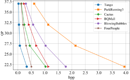
Figure 4 shows the relationship between the QP of the initial frame and the target bit obtained by the block-level multiple QP optimization strategy, where the target bit is in unit of bpp. It can be seen that the relationship between QP and target bits is different for different video sequences. The method we proposed can learn the optimal relationship between QP and target bits under different image complexities by deep learning, and realizes the prediction of the optimal QP for the initial frame. Ultimately, it achieves R-D performance close to that of the multi-QP optimization strategy, while ensuring that the additional complexity of the model meets the requirements for practical use.
The specific implementation process of the algorithm is as follows:
Step 1: Start encoding the sequence, set the target bit rate, and load network weights.
Step 2: Start frame-level bit rate control, perform frame-level bit allocation, then get the current frame’s destination bit allocation at the frame level. Get the current frame’s target bit, and obtain the luminance and chrominance information.
Step 3: Preprocess the brightness and chromaticity information, combine it with the target bit allocated in Step 2, and use a network model to predict the quantization parameter Q1.
Step4: Calculating SATD and estimating the quantization parameter Q2 using the R-(λ) model.
Step 5: If the absolute value of Q1-Q2 is less than the threshold, use Q1 to encode the current frame; otherwise, use Q2 to encode the current frame. In the experiments of this paper, the threshold was set to 5.
4 Experiments
4.I Experimental Setting
We integrated the proposed algorithm into VTM13.0 [24]. The model parameter updating and target bit updating at the frame level are turned off when using the RC to ensure that each frame is encoded as an initial frame. The algorithms are embedded into the VTM using the C + + language in the experiments. The network is trained using GPUs to save training time and tested using the same CPU configuration.
For training, the network was trained using an image dataset to optimize the algorithm for the initial frame. Diversify training data by encoding different images to extract target bits corresponding to different texture features. The RAISE [6] dataset, a real-world dataset with high-resolution uncompressed images, was chosen. 20 images were selected for training, covering four resolutions and a range of texture features from weak to rich, to ensure diverse training data.
For testing, the image was converted to YUV format and then encoded using VTM. Initially, QPs were set to 13 different values ranging from 20 to 40, with increments of 2. The search range for multi-QP optimization was set to -6 to 6. A total of 1040 training samples were collected during the experiment. The encoding results of 22 JVET sequences were used under four different QPs (22,27,32, 37). The encoding configuration used was the AI default, with a frame rate of 50 and an encoding frame interval of 8. A total of 616 test samples were collected for evaluation.
The experiment used the Tensoflow 2.3-Python 3.6 training platform, with Mean Square Error (MSE) as the loss function, to measure the difference between predicted QP and true QP. It is represented as:
where N represents the batch size. yi represents the predicted value of the i-th sample. ŷi represents the true value of the i-th sample. During training, the Adam optimizer was used with a batch size of 32500 training rounds and a learning rate of 10–3.
4.2 R-D Performance
Table 1 shows the R-D performance based on fixed QP, the R-D performance is measured by the Bjontegaard Delta Bit Rate (BDBR) and Bjontegaard Delta Peak Signal to Noise Ratio (BDPSNR) metrics [1]. The anchor in Table 1 is a method of manually setting QP values without enabling bit rate control in VTM13.0. It can be seen that our algorithm closes the gap in R-D performance and the overall BDBR performance is only 0.05%, which is much lower than the 0.38% of VTM13.0. As for BDPSNR performance, the proposed method with -0.03dB also outperforms VTM13.0 with -0.04dB. As for the multi-QP optimization, it only improves the fixed QP R-D performance by 0.08%, but the multi-QP optimization strategy consumes a significant amount of coding time.
In Table 2, we also shows the R-D performance of our algorithm compared to VTM13.0 RC. From the table, the BDBR and BDPSNR are -0.25% and 0.015dB. It also indicates that the proposed method outperforms VTM13.0.
R-D performance of the methods on VTM13.0.
| Category | Sequence | VTM13.0 [24] | Multi QP optimization | Ours | |||
|---|---|---|---|---|---|---|---|
| BDPSNR (dB) | BDBR (%) | BDPSNR (dB) | BDBR (%) | BDPSNR (dB) | BDBR (%) | ||
| Tango | 0.10 | -3.90 | 0.01 | -0.60 | -0.03 | 1.88 | |
| A1 | FoodMarket4 | -0.02 | 1.09 | 0.01 | -0.87 | -0.03 | 1.04 |
| Campfire | -0.17 | 6.45 | 0.01 | -0.64 | -0.10 | 3.59 | |
| Average | -0.03 | 1.21 | 0.01 | -0.70 | -0.06 | 2.17 | |
| CatRobot | -0.02 | 0.47 | 0.01 | -0.36 | -0.03 | 0.99 | |
| A2 | DaylightRoad2 | 0.17 | -14.94 | -0.02 | 3.71 | 0.22 | -17.31 |
| ParkRunning3 | 0.05 | -0.80 | 0.05 | -0.80 | 0.06 | -1.06 | |
| Average | 0.06 | -5.09 | 0.01 | 0.85 | 0.09 | -5.79 | |
| BasketballDrive | -0.02 | 0.75 | 0.01 | -0.52 | -0.02 | 0.19 | |
| BQTerrace | -0.09 | 1.42 | 0.01 | -0.13 | -0.04 | 0.46 | |
| B | Cactus | -0.07 | 1.86 | 0.01 | -0.33 | -0.05 | 1.47 |
| Kimono1 | -0.04 | 1.20 | 0.01 | -0.31 | -0.03 | 0.72 | |
| ParkScene | -0.08 | 1.93 | 0.01 | -0.21 | -0.04 | 0.84 | |
| Average | -0.06 | 1.43 | 0.01 | -0.30 | -0.03 | 0.74 | |
| BasketballDrill | -0.08 | 1.61 | 0.00 | -0.03 | -0.07 | 1.43 | |
| BQMall | -0.05 | 0.88 | 0.00 | -0.03 | -0.05 | 0.79 | |
| C | PartyScene | -0.08 | 0.98 | 0.00 | 0.03 | -0.04 | 0.58 |
| RaceHorses | -0.14 | 2.07 | 0.01 | -0.14 | -0.05 | 0.50 | |
| Average | -0.09 | 1.39 | 0.00 | -0.04 | -0.05 | 0.83 | |
| BasketballPass | -0.02 | 0.34 | 0.02 | -0.25 | -0.01 | 0.16 | |
| BlowingBubbles | -0.07 | 1.04 | 0.00 | 0.06 | -0.05 | 0.75 | |
| D | BQSquare | -0.11 | 1.42 | -0.01 | 0.03 | -0.09 | 1.23 |
| RaceHorses | -0.08 | 1.19 | 0.00 | -0.04 | -0.08 | 1.10 | |
| Average | -0.07 | 0.99 | 0.00 | -0.05 | -0.06 | 0.81 | |
| FourPeople | -0.07 | 1.30 | 0.00 | -0.04 | -0.05 | 0.82 | |
| E | Johnny | -0.04 | 1.04 | 0.01 | -0.26 | -0.02 | 0.47 |
| KristenAndSara | -0.05 | 0.88 | 0.01 | -0.14 | -0.02 | 0.37 | |
| Average | -0.05 | 1.07 | 0.01 | -0.15 | -0.03 | 0.55 | |
| Overall Average | -0.04 | 0.38 | 0.01 | -0.08 | -0.03 | 0.05 | |
4.3 Bit Control Error
This section evaluates the bit CE performance of the proposed algorithm. The CE represents the difference between the allocated bits and the actual consumed bits. The CE is calculated as follows:
where Re denotes the number of allocated bits and Rt denotes the actual number of coded bits consumed.
Table 3 shows the detailed performance of the proposed algorithm and VTM13.0 RC algorithm in controlling errors. It can be seen that the algorithm proposed in this article has smaller CEs in the vast majority of sequences. Overall, the algorithm reduces the error of the original encoder from 10.74% to 7.19%. It is worth mentioning that the proposed algorithm reduces the CE by an average of 6.77% on the 4K sequence, which is in line with the current demand for high-resolution sequences.
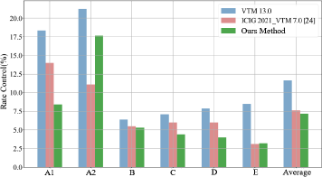
Figure 5 shows the comparison results of the algorithm in this paper with VTM13.0 RC and Huang et al. [8] in terms of CE. In Huang et al. [8], the feature extraction and machine learning methods were used to represent image complexity. From Figure 6, it can be seen that compared with the VTM13.0 RC algorithm, our algorithm reduces its CE in all categories; Compared with the CE performance of Huang et al. [8], the average CE of our algorithm is 7.16%, which is better than its CE of 7.62%.
CE performance of the methods.
| Category | Sequence | VTM13.0(%) [24] | Ours(%) |
|---|---|---|---|
| Tango | 30.75 | 18.62 | |
| A1 | FoodMarket4 Campfire | 17.09 7.28 | 7.87 8.88 |
| Average | 18.37 | 8.38 | |
| CatRobot | 17.05 | 18.93 | |
| A2 | DaylightRoad2 | 42.59 | 31.47 |
| ParkRunning3 | 4.09 | 2.63 | |
| Average | 21.24 | 17.68 | |
| BasketballDrive | 10.16 | 14.23 | |
| BQTerrace | 8.74 | 3.09 | |
| B | Cactus Kimono1 | 7.56 4.35 | 3.39 4.80 |
| ParkScene | 1.11 | 1.06 | |
| Average | 6.38 | 5.31 | |
| C | BasketballDrill | 3.93 | 3.91 |
| BQMall | 5.41 | 5.46 | |
| PartyScene | 2.87 | 5.84 | |
| RaceHorses | 16.1 | 2.33 | |
| Average | 7.08 | 4.39 | |
| D | BasketballPass | 4.47 | 3.34 |
| BlowingBubbles | 10.01 | 2.59 | |
| BQSquare | 13.39 | 7.25 | |
| RaceHorses | 3.71 | 2.85 | |
| Average | 7.90 | 4.01 | |
| FourPeople | 8.77 | 3.12 | |
| E | Johnny | 9.22 | 3.57 |
| KristenAndSara | 7.56 | 2.85 | |
| Average | 8.52 | 3.18 | |
| Overall Average | 10.74 | 7.19 |
4.4 Ablation Experiments
We performed ablation experiments on various feature selection methods to verify the effectiveness of the extracted features. The results from Table 4 indicate that training with all the features provides the most accurate results. Brightness is a crucial feature because it is not downsampled and contains abundant texture information. On the other hand, the importance of chromaticity is relatively less significant because of the repetitive information between chromaticity and brightness. Furthermore, chromaticity can interfere with the regressor’s judgment in decision trees and AdaBoost machine learning methods. It is important to consider the target bit rate during network training, as models that do not incorporate it during training tend to lose their predictive ability.
Feature selection and ablation results for machine learning models and our network.
| Model | All features | Excluding V component | Excluding U component | Excluding chromaticity component | Excluding brightness component | Excluding target bit rate |
|---|---|---|---|---|---|---|
| Decision Tree | 7.880 | 7.767 | 7.706 | 6.631 | 8.782 | 58.495 |
| Random Forest | 2.655 | 2.841 | 2.840 | 3.044 | 3.882 | 49.978 |
| AdaBoost | 7.865 | 7.439 | 7.666 | 7.684 | 11.070 | 36.897 |
| Bagging | 3.288 | 3.533 | 3.538 | 3.812 | 4.919 | 51.176 |
| Ours | 1.064 | 1.659 | 1.872 | 2.497 | 1.913 | 36.284 |
4.5 Further Analysis
Table 5 presents the additional encoding time required of the methods. This additional time is measured relative to the encoding duration controlled by the VTM raw bit rate, serving as a benchmark for comparison. When compared to the four machine learning algorithms reported in other literature, our proposed algorithm introduces only a 4.18% increase in encoding time. Notably, the majority of this additional time is attributed to preprocessing.
Thanks to the lightweight design of the network, the additional encoding time of the algorithm accounts for a small proportion. Through experiments, we obtained the proportion of feature extraction time and network forward propagation time in the additional encoding time of the algorithm. It can be seen that feature extraction operations occupy the vast majority of additional encoding time. This is because feature preprocessing requires extracting multiple global and local features. The proportion of forward propagation time in the network is very small, because the preprocessing operation results in the input feature map of the network being only a matrix of size 4@4×3, making the forward propagation speed of the network extremely fast.
To validate the efficacy of our proposed method, we trained both standard machine learning classifiers and our method using the extracted training data. Features were flattened and the target bit rate appended for predictions. Classification accuracy was the evaluation metric. To ensure fair comparisons, we used identical software, hardware, and frameworks (OpenCV) for testing. Table 6 compares our method’s performance to the classifiers, revealing a slight increase in forward propagation time but significantly higher accuracy. This justifies the added computational cost.
Classification accuracy and time consuming performance.
| Model | Classification Accuracy (%) | Usage Time (us) |
|---|---|---|
| Logistic Regression | 20.41 | 1001.36 |
| K-Nearest Neighbor Algorithm | 31.02 | 1999.38 |
| Random Forest | 42.55 | 1000.88 |
| SVM | 41.22 | 2000.09 |
| Boosting | 19.59 | 1000.64 |
| Ours | 49.18 | 4016.64 |
In summary, the algorithm improves the overall R-D performance and narrows the performance gap between the original encoder RC and the multi QP optimization strategy. Compared with relevant literature algorithms and multi QP optimization strategies, the additional cost of our algorithm is smaller; Compared with machine learning methods, the algorithm has a higher accuracy while consuming more acceptable prediction time.
5 Conclusion
This paper proposes a learned-based initial frame QP prediction algorithm. Firstly, this paper explains the key to determining the initial frame QP through theoretical and statistical experiments, and demonstrates the shortcomings of current VVC in representing image complexity through statistical experimental results. Secondly, this article builds a lightweight QP prediction residual network, which represents the complexity of the image from rough to detailed through preprocessing and residual modules, and combines target bits to achieve QP prediction. Finally, the experimental section demonstrated through algorithm comparison that the proposed algorithm has good performance in controlling errors, R-D performance, and additional algorithm complexity. The rationality of network design and the effectiveness of feature selection was also demonstrated through ablation experiments.

