


The implicit neural representation (INR) employed in image compression shows high decoding efficiency, yet it requires long encoding times due to the need for the model training tailored to the specific image being coded. Thus, we propose a new image compression scheme leveraging the 2D Gaussian splatting technique to accelerate encoding speed and maintain decoding efficiency. Specifically, we parameterize these Gaussians with key attributes including position, anisotropic covariance, color, and opacity coefficients, totaling 9 parameters per Gaussian. We initialize these Gaussians by sampling points from the image, followed by employing an α-blending mechanism to determine the color values of each pixel. For compact attribute representation, we adopt a K-means based vector quantization approach for anisotropic covariance, color and opacity coefficients. Additionally, we introduce an adaptive dense control methodology to dynamically adjust Gaussian numbers, facilitating automatic point reduction or augmentation. Finally, the position, codebooks and indexes of other attributes are quantized and compressed by the lossless entropy coding. Our experimental evaluation demonstrates that our method achieves faster encoding speeds compared to other INR techniques while exhibiting comparable decoding speeds. The source code is available via the following link: https://github.com/ppingzhang/2DGS_ImageCompression.
1 Introduction
In environments characterized by massive image generation, image compression is essential for conserving storage space and bandwidth. Various codecs have been developed to optimize reconstruction quality within bitrate constraints. There are three types of image compression methods: conventional transformbased image compression methods [31,4], explicit learning based methods [3,8] and implicit learning based methods [19,6].
The conventional transform-based image compression pipelines, e.g., JPEG, HEVC (High-Efficiency Video Coding) [31] and VVC (Versatile Video Coding) [4], consist of essential modules, such as transform, quantization, and entropy coding. However, these codecs suffer from drawbacks such as blockbased partitioning, which leads to blocking artifacts, and complex inter-module dependencies that hinder joint optimization. With the rapid progress of deep learning, many researchers [3,8] have looked into using neural networks to build image compression systems that are optimized end-to-end. In these explicit representation approaches, the whole system can be improved together, boosting performance across all parts and ultimately enhancing the overall outcome. Subsequently, implicit neural representation has been employed in numerous image compression methods to decrease computational complexity and enhance decoding time in deep-based image compression [11,29]. Initial endeavors employing Implicit Neural Representation (INR) for image compression entail the training and quantization of individual SIREN networks for each image [11]. The COOL-CHIC framework [19] incorporates a lightweight Multilayer Perceptron (MLP) decoder, along with latent representations, to achieve a reduced decoder complexity. INRs are to learn an implicit continuous mapping using a learnable neural network. Thus, the encoding process is frequently deemed to be time-consuming [6].
3D Gaussian representation combines the advantages of explicit and implicit representation, offering a flexible and expressive framework for encapsulating 3D scenes [18]. This novel method enables real-time, high-quality rendering of radiance fields in a wide variety of scenes, with training times comparable to the fastest previous techniques. Building upon this foundation, we introduce a new approach inspired by the principles of the 3D Gaussian representation: 2D Gaussian splatting for image compression.
Different from a typical 3D Gaussian, which consists of 59 learnable parameters [18], our proposed method simplifies the parameters of the 2D Gaussian. It includes only four attributes (equivalent to a total of 9 parameters): position, anisotropic covariance, color and opacity coefficients. An α-blending mechanism is employed to calculate the value for each pixel. Here, we use the adjustive dense control algorithm to dynamically adjust the number of Gaussians [18]. Using more 2D Gaussians usually improves image quality, but it can also increase bitrates. Due to the similarity of the covariance matrix, we employ a K-means algorithm during training for vector quantization to attain a compact representation. Similarly, due to the lower sensitivity of opacity, color and opacity values are encapsulated in a vector to facilitate K-means based vector quantization. This method involves storing parameter codebooks alongside corresponding indices for each Gaussian, leading to significant reductions in storage requirements for 2D Gaussians. Furthermore, for a more compact representation of the parameters, we employ post-training quantization. This approach allows us to adjust the precision of both the cookbook and position without the fine-tuning procedure. In comparison to INR-based codecs such as COIN [11] and WIRE [28], our method demonstrates faster encoding speed while maintaining comparable decoding speed. In particular, our model outperforms JPEG in reconstruction quality at low bitrates.
2 Related Work
2.1 Image Compression
Image compression aims to represent image signals compactly for efficient transmission and storage. Over the past decades, numerous image compression standards have been developed, such as JPEG [32], JPEG2000 [27], HEVC (Intra)[30,38], and VVC (Intra) [4]. These standards commonly employ prediction, transform coding, and entropy coding methods to diminish redundancies in images.
Learning-based image compression has made significant strides in compression efficacy, highlighting the potential of neural networks to nonlinearly represent visual signals, consequently boosting compression efficiency [2,1]. Researchers have been exploring various possibilities for the transform module in image compression [2,3,34,22,34,35]. Variational Autoencoder (VAE) models have garnered significant attention in the research community due to their notable performance and architectural robustness [2,3,7]. However, despite these advancements, a persistent challenge remains unaddressed: the issue of slow decoding speed, particularly evident in codecs utilizing the con-volutional autoencoder framework [8,17,34]. Despite numerous attempts to ameliorate this limitation through various techniques, such as the checkboard structure [16], these codecs continue to exhibit comparatively slower decoding speeds when compared with traditional codecs.
2.2 Implicit Neural Representation for Compression
INR has attracted considerable interest due to its capability to model diverse signals. This is accomplished by parameterizing a signal through a function that synthesizes desired properties from given inputs. As a result, the signal becomes implicitly encoded within the parameters of the network.
In image compression, INR has emerged as a promising approach that harnesses the power of neural networks to compress and decompress images without explicitly encoding pixel values [29,6]. Strumpler et al. [29] introduced meta-learned initializations for INR-based compression, aiming to enhance rate-distortion performance. They subsequently proposed a straightforward yet highly effective modification to the network architecture compared to prior works. Dupont et al. [11] presented the COIN model, which stores the weights of an overfitted neural network rather than RGB values for each pixel in an image. Additionally, they developed COIN++, an advanced neural compression framework adept at handling a diverse array of data modalities [12]. In the realm of video compression, there have been notable strides in INR-based video compression schemes. Chen et al. [6] introduced an innovative neural representation for videos known as NeRV. This method encodes videos within neural networks, offering a novel approach to video compression. Subsequently, they proposed a hybrid neural representation for storing videos. This approach provides decoding advantages in terms of speed and flexibility compared to conventional codecs.
2.3 3D Gaussian Splatting
3D Gaussian Splatting (3DGS) [18] has demonstrated superior quality and faster rendering capabilities. However, its primary drawback lies in the increased storage requirements compared to NeRF (Neural Radiance Fields) methods [25,33], potentially restricting its applicability in various settings. Consequently, numerous efforts [20,13] have been made to preserve the quality and rapid rendering speed of the 3DGS method while reducing model storage requirements. Numerous Gaussians often exhibit similarity in their parameters. Based upon this observation, Navaneet et al. [24] propose a straightforward vector quantization technique leveraging the K-means algorithm for parameter quantization. Then, the parameters of each Gaussian are represented in a compact codebook alongside the corresponding indices. Lee et al. [20] proposed a compact 3DGS model to diminish the Gaussian points and compress the Gaussian attributes effectively. Navaneet et al. [24] introduced a novel compressed 3D Gaussian splat representation technique employing sensitivity-aware vector clustering alongside quantization-aware training to compress Gaussian parameters effectively. Zhang et al. [36] introduced a 2D Gaussian representation for images, showcasing its ability to achieve rapid decoding speeds. The main difference between us lies in the quantization method. Our method utilizes K-means based vector quantization for covariance and color, respectively. This allows for updates during training, enabling consideration of quantization errors in the training process. In contrast, GaussianImage employs a two-step compression procedure. After the image is overfitted, GaussianImage requires attribute quantization-aware fine-tuning.
2.4 Model Compression
After obtaining INR, another key issue is model compression as models govern the bitstream. Model compression aims to reduce the size and complexity of neural networks [21,10]. Notably, model pruning seeks to eliminate redundant layers from neural networks [9,14]. Weight quantization, another key method, involves reducing the precision of weights and activations within the model [37,26]. Similarly, knowledge distillation entails training a compact student model to emulate the behavior of the original teacher model [14,15]. Weight quantization stands out as a fundamental component of model compression. This technique typically involves decreasing the precision of numerical values by representing them with fewer bits, achieved through methods such as fixed-point quantization and dynamic range quantization [6,5].
3 Approach
3.1 Overview
The workflow of the proposed model is illustrated in Figure 1. Specifically, we initialize these Gaussians by the sampled points from the image, which consists of 4 attributes: position, anisotropic covariance (scale and rotation), color coefficients, and opacity, resulting in a total of 9 parameters per Gaussian. To represent these parameters compactly, we employ the K-means based vector quantization approach. This involves designing a codebook for the anisotropic covariance Σ, which includes both scale and rotation. For color and opacity, we amalgamate them into a vector Vc that shares the same codebook. Subsequently, we utilize an α-blending mechanism to determine the color values of each pixel. Then, an adaptive dense control methodology is implemented to dynamically adjust the quantity of Gaussians, facilitating automatic point reduction or augmentation. Furthermore, the model minimizes the loss between the ground truth and the blended value. This loss function comprises an 𝓁1 loss and a Structural Similarity Index (SSIM) loss, ensuring comprehensive optimization of the entire model. After training, the codebook and indexes of Vs and Vc, and the position parameter μ are quantized and compressed into the bit stream. During the decoding phase, the bitstream is decompressed and dequantized to obtain the decoded attributes of 2D Gaussiane, which are then blended to generate the decoded image.

The workflow of the proposed scheme. It includes sampling and initialization, K-means based vector quantization, α-blending, and adaptive dense control processes.
The workflow of the proposed scheme. It includes sampling and initialization, K-means based vector quantization, α-blending, and adaptive dense control processes.
3.2 Differentiable 2D Gaussian splatting
2D Gaussian is a basic image representation unit, which can be parameterized by its position μ ∈ ℝ2 and covariance matrices Σ ∈ ℝ2×2 in the 2D space, as follows:
where d = x – μ, which is the displacement between the pixel center and the center of the 2D Gaussian. Since the covariance matrix needs to be positive definite, it is factored into a rotation matrix R ∈ ℝ2×2 and scaling matrix S ∈ ℝ2×2 as Σ = RSSTRT for easier optimization [18], where the rotation matrix R and the scaling matrix S are expressed as
and
Here, θ represents the rotation angle, s1 and S2 are the scaling factors in different eigenvector directions.
For each Gaussian, denoted by Gi, where i represents its index, we establish a default order to perform the α-blending. Thus, the color value of a pixel (C) is computed by blending all N 2D Gaussiane contributing to this pixel according to the formula:
where the variable α is computed using the 2D covariance Σ and opacity oi:
3.3 Quantization
K-means based vector quantization. In this model, a significant challenge arises from the necessity of employing numerous Gaussians to accurately represent images, with each Gaussian characterized by 9 parameters, resulting in considerable storage requirements. Consequently, this approach proves inefficient for certain applications, particularly those deployed on edge devices. In addition, it is common for 2D Gaussians to exhibit similarities in their parameter values, such as covariance or color. To efficiently represent these Gaussians while minimizing redundancy, vector quantization coupled with the K-means algorithm is employed for attribute quantization.
We combine scaling and rotation parameters into a vector Vs ∈ RN×3, which represents the covariance. Similarly, due to the lower sensitivity of opacity, color and opacity values are encapsulated in a vector Vc ∈ RN×4. Each vector serves as the fundamental unit in the K-means algorithm. Specifically, we cluster Vs and Vc into k clusters, respectively. These vectors can be represented using k vectors of size d along with N integer indices. Given that N >> k, this approach offers substantial compression ratios. To minimize errors, we update the centroids at each iteration following the K-means algorithm. Here, the K-means optimization process empirically iterates through 10 iterations. Parameter quantization. To further compactly represent the parameter, we utilize post-training quantization (PTQ) [6], which enables us to adjust the precision of the cookbook and position without the fine-tuning procedure. The formula for quantization is presented below:
In this context, the term |*] signifies the process of rounding a given value to the nearest integer. The variable “b” denotes the bit length for the quantized model, while θmax and θmin represent the maximum and minimum values of the parameter tensor θ respectively. The scaling factor is denoted by the variable S, and each parameter can be assigned a value based on (7) and (8). Following parameter quantization, we employ Arithmetic coding, a lossless compression method, to compress the quantized parameters. Due to the sensitivity of Gaussians to position, we empirically set them to 10 bits, while other parameters are selected optimally under different bit lengths.
3.4 Adaptive dense control
Inspired by the adaptive dense control method [18], we augment the Gaussians within both the under-reconstruction and over-reconstruction regions. In this context, the under-reconstruction region encompasses small Gaussians characterized by limited coverage. These Gaussians can be effectively managed by replicating them at the same scale and adjusting their position along the directional gradient. In contrast, the over-reconstruction region refers to large Gaussians with significant coverage. We replace these Gaussians with two new ones, scaling them down by a factor. These Gaussians can be identified through positional gradients, as they correspond to regions that are still inadequately reconstructed, prompting the optimization process to make necessary adjustments to the Gaussians. Meanwhile, we regularly remove Gaussians with o values less than ϵo, where ϵo is empirically set to 0.001.
4 Experiments
4.1 Training Data
We conducted experiments on the Kodak image dataset, which comprises 24 images with the size of 768 × 512. We evaluate our model against three deep image codecs, including Balle et al.’s model [3], Minnen et al.’s model [23], and Cheng et al.’s model [8]. We also compare against the JPEG, BPG and VTM image codecs. Furthermore, we compare with the implicit neural network, COIN [11]. To benchmark our model, we leverage the CompressAI library along with its pre-trained models. We implement our model in PyTorch and perform all experiments on a single RTX3090 GPU.
4.2 Comparison Results
The results of this evaluation across various bits per pixel (bpp) levels are depicted in Figure 2. It is evident that our model outperforms JPEG at low bitrates. The visual quality comparison is depicted in Figure 3. Decoded images from JPEG display noticeable blocking artifacts, whereas those from our model showcase superior reconstruction performance at low bit rates. Besides, we display all results in the Kodak dataset as shown in Table. While our approach does not yet reach the level of state-of-the-art compression methods, we consider its performance promising for future advancements in this direction.
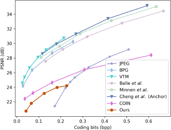
Performance comparison of our approach and different baselines on Kodak dataset in PSNR.
Performance comparison of our approach and different baselines on Kodak dataset in PSNR.
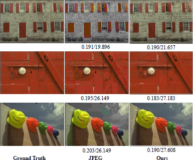
Visual quality comparison of different methods on Kodak dataset. The values below each image are coding bits(bpp)/PSNR(dB) values, where a higher PSNR value represents better signal quality.
Visual quality comparison of different methods on Kodak dataset. The values below each image are coding bits(bpp)/PSNR(dB) values, where a higher PSNR value represents better signal quality.
The result (PSNR and bpp) of every image in Kodak dataset.
| Images | PSNR | bpp | PSNR | bpp | PSNR | bpp | PSNR | bpp |
|---|---|---|---|---|---|---|---|---|
| kodim01 | 19.193 | 0.042 | 19.869 | 0.064 | 21.029 | 0.126 | 21.962 | 0.190 |
| kodim02 | 24.861 | 0.043 | 25.706 | 0.067 | 26.790 | 0.124 | 27.183 | 0.183 |
| kodim03 | 23.226 | 0.043 | 24.506 | 0.066 | 26.470 | 0.130 | 27.608 | 0.190 |
| kodim04 | 22.099 | 0.043 | 24.055 | 0.068 | 25.273 | 0.125 | 26.539 | 0.186 |
| kodim05 | 16.625 | 0.040 | 17.541 | 0.067 | 18.702 | 0.120 | 19.574 | 0.174 |
| kodim06 | 21.032 | 0.043 | 21.191 | 0.066 | 22.455 | 0.123 | 22.853 | 0.179 |
| kodim07 | 20.448 | 0.043 | 21.272 | 0.067 | 23.175 | 0.121 | 24.341 | 0.179 |
| kodim08 | 15.433 | 0.041 | 16.125 | 0.064 | 17.657 | 0.119 | 18.391 | 0.175 |
| kodim09 | 21.593 | 0.041 | 22.914 | 0.065 | 24.800 | 0.121 | 25.841 | 0.180 |
| kodim10 | 22.109 | 0.042 | 23.232 | 0.067 | 25.022 | 0.125 | 25.898 | 0.178 |
| kodim11 | 20.719 | 0.041 | 21.786 | 0.068 | 22.956 | 0.128 | 23.728 | 0.188 |
| kodim12 | 22.549 | 0.043 | 24.220 | 0.068 | 26.167 | 0.125 | 27.330 | 0.184 |
| kodim13 | 17.762 | 0.042 | 18.256 | 0.066 | 18.857 | 0.128 | 19.207 | 0.184 |
| kodim14 | 19.483 | 0.042 | 20.118 | 0.063 | 21.566 | 0.125 | 22.096 | 0.189 |
| kodim15 | 20.954 | 0.041 | 22.809 | 0.065 | 24.864 | 0.123 | 25.880 | 0.185 |
| kodim16 | 24.156 | 0.042 | 25.015 | 0.066 | 25.979 | 0.130 | 26.433 | 0.182 |
| kodim17 | 22.174 | 0.042 | 23.264 | 0.068 | 24.707 | 0.128 | 25.540 | 0.189 |
| kodim18 | 19.971 | 0.040 | 20.712 | 0.066 | 21.362 | 0.121 | 21.980 | 0.178 |
| kodim19 | 19.758 | 0.043 | 20.999 | 0.067 | 22.302 | 0.127 | 23.033 | 0.183 |
| kodim20 | 20.158 | 0.043 | 22.133 | 0.066 | 23.936 | 0.125 | 25.103 | 0.185 |
| kodim21 | 19.955 | 0.042 | 21.009 | 0.066 | 21.876 | 0.121 | 22.692 | 0.188 |
| kodim22 | 22.034 | 0.044 | 22.819 | 0.066 | 23.825 | 0.123 | 24.641 | 0.178 |
| kodim23 | 22.107 | 0.040 | 23.609 | 0.067 | 25.099 | 0.130 | 26.152 | 0.189 |
| kodim24 | 19.242 | 0.043 | 20.066 | 0.065 | 21.065 | 0.129 | 21.634 | 0.183 |
| Average | 20.735 | 0.042 | 21.801 | 0.066 | 23.164 | 0.125 | 23.985 | 0.183 |
4.3 Runtime Efficiency
Table 2 presents the computational complexity of various image codecs evaluated on the Kodak dataset. Notably, our model demonstrates superior speed in the encoding phase compared to COIN [11] and WIRE [28]. Furthermore, the decoding speed of our proposed model outperforms that of the majority of deep learning-based codecs, e.g., Balle et al.’s and Minnen et al.’s models.
4.4 Ablation Studies
We conducted ablation studies on the loss function, comparing our proposed scheme (𝓁1 + SSIM) against using only the 𝓁1 loss function. The results are presented in Table 3, demonstrating that our proposed scheme outperforms the 𝓁1 loss function alone.
Moreover, we examined the impact of different k settings in the K-means based vector quantization, as shown in Table 3. Our approach incorporates adaptive k parameters, wherein larger k values are utilized for high bit rates, while smaller k values are employed for low bit rates. Comparative analysis against fixed k settings reveals that our proposed scheme consistently achieves enhanced performance.
The comparison results of the encoding, decoding time, and model size on Kodak dataset.
| Models | Encoding time | Decoding time | Model size (K) |
|---|---|---|---|
| JPEG | 0.0195 | 0.0193 | – |
| BPG | 2.0338 | 0.1174 | – |
| VTM | 80.7570 | 0.1230 | – |
| Balle et al. | 0.0474 | 0.0431 | 19827.5117 |
| Minnen et al. | 3.1228 | 6.2187 | 55197.1367 |
| Cheng et al. | 4.4117 | 6.3423 | 46223.2383 |
| WIRE | 424.8000 | 0.0024 | 65.4033 |
| COIN | 336.6627 | 0.0011 | 7.2120 |
| Ours | 250.4321 | 0.0224 | 6.8664 |
5 Conclusion
In this paper, we introduce 2D Gaussian splatting as a new technique for image compression. Our experimental results demonstrate that this approach can outperform JPEG at low bit-rates. Additionally, our model showcases notably faster encoding speeds compared to INR-based image codecs, such as CION and WIRE. We anticipate that continued research in this domain will yield a new class of methods for neural data compression, offering promising avenues for further exploration. Additionally, we aim to enhance both the encoding and decoding speeds through CUDA programming.
Acknowledgments
This work was supported in part by the Hong Kong Innovation and Technology Commission (InnoHK Project CIMDA), in part by the General Research Fund of the Research Grant Council of Hong Kong under Grants 11209819, 11203820, and 11203220, in part by ITF Project GHP/044/21SZ, and in part by CityU Applied Research Grant 9667255.

