


This study aims to examine what underlies the estimated relation between idiosyncratic volatility and realized return.
Idiosyncratic volatility has a dual effect on stock pricing: it not only affects investors' expected return but also affects the efficiency of stock price in reflecting its value. Therefore, the estimated relation between idiosyncratic volatility and realized return captures its relations with both expected return and the mispricing-related component due to its dual effect on stock pricing. The sign of its relation with the mispricing-related component is indeterminate.
The estimated relation between idiosyncratic volatility and realized return decreases and switches from positive to negative as the estimation sample consists of proportionately more ex ante overvalued observations; it increases and switches from negative to positive as the estimation sample consists of proportionately more ex post overvalued observations. In sum, the relation of idiosyncratic volatility with the mispricing-related component dominates its relation with expected return in its estimated relation with realized return. Moreover, its estimated relation with realized return varies with research design choices and even switches sign due to their effects on its relation with the mispricing-related component.
The novelty of the study is evident in the implication of its findings that one cannot infer the sign of the relation of idiosyncratic volatility with expected return from its estimated relation with realized return.
1. Introduction
Whether a stock's expected return depends on idiosyncratic volatility is an unresolved asset pricing puzzle (Hou & Loh, 2016). Traditional asset pricing theories predict either no relation between idiosyncratic volatility and expected return under the assumption of complete and frictionless markets and perfect portfolio diversification (Black, 1972; Lintner, 1965; Sharpe, 1964) or a positive relation under the assumption of limited portfolio diversification (Levy, 1978; Merton, 1987). However, Ang, Hodrick, Xing and Zhang (2006) and several following studies find a negative relation between idiosyncratic volatility and realized return. If realized return is an adequate expected return proxy, considered an asset pricing puzzle, the finding of a negative relation between idiosyncratic volatility and realized return poses a direct challenge to those asset pricing theories.
Existing research has focused on proposing explanations for the negative relation and on evaluating the proposed explanations (Hou & Loh, 2016) [1]. This focus downplays the fact that quite a few studies find a positive or no relation between idiosyncratic volatility and realized return (e.g. Fama & MacBeth, 1973; Lehmann, 1990). That is, findings about the relation between idiosyncratic volatility and realized return are indeed inconsistent across studies. Moreover, some studies with inconsistent findings employ highly overlapped samples and similar – or even identical – measures and testing methods. Arguably, what drives this inconsistency is just as puzzling as the finding of a negative relation.
Evidently, research is needed to investigate what drives this inconsistency. Answers to this question help to resolve the idiosyncratic volatility puzzle. We aim to shed light on this inconsistency. To do so, we first show that the dual effect of idiosyncratic volatility on stock pricing causes its estimated relation with realized return to be an inadequate indicator of its relation with expected return. Idiosyncratic volatility has a dual effect on stock pricing because it affects both investors' expected return and the efficiency of stock price in reflecting its underlying value. Idiosyncratic volatility is positively related to arbitrage risks that deter arbitrage and thus hinder the reduction of mispricing (Pontiff, 2006). In sum, idiosyncratic volatility has a dual effect on stock pricing because it not only shapes investors' expected return but also lowers stock pricing efficiency.
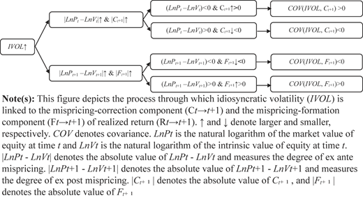
Due to this dual effect, the estimated relation of idiosyncratic volatility (IVOL) with realized return () captures its relations with both expected return and with the mispricing-related component of . In principle, the mispricing-related component stems from the correction of ex ante mispricing () or from the formation of ex post mispricing () or from both. For the correction of ex ante undervaluation, is positive and increases with the degree of ex ante undervaluation corrected, while for the correction of ex ante overvaluation, is negative and decreases with the degree of ex ante overvaluation corrected; for the formation of ex post undervaluation, is negative and decreases with the degree of ex post undervaluation formed, while for the formation of ex post overvaluation, is positive and increases with the degree of ex post overvaluation formed. Because IVOL is positively related to arbitrage risks, it is positively related to the degree of mispricing, both ex ante and ex post. Taken together, evidently IVOL is positively related to among ex ante undervalued stocks and negatively related to among ex ante overvalued stocks since a higher value of IVOL is associated with greater ex ante mispricing, both undervaluation and overvaluation; and it is negatively related to among ex post undervalued stocks and positively related to among ex post overvalued stocks, since a higher value of IVOL is associated with greater ex post mispricing, both undervaluation and overvaluation. Figure 1 depicts the process through which IVOL is linked to and .
Idiosyncratic volatility and the mispricing-related component
Idiosyncratic volatility and the mispricing-related component
Figure 1 shows that IVOL's relation with is a potentially biased estimate of its relation with expected return due to its relations with and . To infer IVOL's relation with expected return from its estimated relation with , the crucial task is to calibrate the sign and magnitude of its relation with the mispricing-related component ( and ). However, this task is empirically unfeasible because all estimates of value are noisy and thus “we can never know how far away price is from value” (Black, 1986, p. 533). Nevertheless, IVOL's relations with and suggest a testable hypothesis that, ceteris paribus, its estimated relation with decreases with the proportion of ex ante overvalued observations in the sample and increases with the proportion of ex post overvalued observations in the sample.
Consistent with the hypothesis, we find robust evidence that IVOL's estimated relation with decreases and switches sign from positive to negative as the estimation sample consists of proportionately more ex ante overvalued observations and increases and switches sign from negative to positive as the estimation sample consists of proportionately more ex post overvalued observations. Our finding suggests that we cannot draw a reliable inference about IVOL's relation with expected return from its estimated relation with . Indeed, the sign switching for IVOL's estimated relation with suggests that its relations with and dominate its relation with expected return in its estimated relation with . If not, one would not observe such sign switching other than in the virtually inconceivable situation that its relation with expected return varies similarly in response to change in the proportion of ex ante (ex post) overvalued observations in the sample. One thus cannot infer the sign – let alone the magnitude – of IVOL's relation with expected return from its estimated relation with . Evidently, the documented negative relation between IVOL and does not necessarily contradict the predictions of traditional asset pricing theories and hence may not be an asset pricing puzzle. Moreover, we show that existing methods cannot address the bias. In sum, the estimated relation of idiosyncratic volatility (IVOL) with realized return () is an inadequate indicator of its relation with expected return.
Our findings demonstrate that IVOL's estimated relation with is inherently unstable due to the nonlinearity of its relations with and . We reason that ostensibly immaterial variation in research design choices can cause IVOL's estimated relation with to vary dramatically and even switch sign due to their effects on its estimated relations with and . First, a research design choice can change the proportions of ex ante and ex post undervalued and overvalued observations in the sample. Second, it can change the weight of ex ante significantly undervalued observations and ex post significantly overvalued observations in IVOL's estimated relation with due to its effect on the distribution of . A well-known regularity about is that it is right-skewed. We show that large positive returns driving the right-skewness of stem from the correction of ex ante significant undervaluation and the formation of ex post significant overvaluation to a large extent. This is not surprising because for the correction of ex ante undervaluation and for the formation of ex post overvaluation can be very large, whereas for the correction of ex ante overvaluation and for the formation of ex post undervaluation are at most −1.
We show that IVOL's estimated relation with is sensitive to ostensibly immaterial variation in oft-employed research design choices in a predictable manner consistent with our reasoning. Prior studies have generally excluded observations with very low price, arguing that the price movements of those stocks are susceptible to microstructure biases. However, these studies may differ regarding the price threshold for exclusion. Moreover, these studies rarely specify the timing for measuring stock price. We show that IVOL's estimated relation with varies dramatically and even switches sign in a predictable manner in response to ostensibly immaterial variation in the price threshold for exclusion ($0 vs $1 vs $5) and in the timing of measuring stock price (at the beginning and at the end of the holding period and average stock price for the holding period). Prior studies may also exclude small stocks, arguing that data quality of those stocks is low due to their illiquidity and ensuing noise in their stock pricing and that their economic significance is trivial. In practice, studies have great discretion over the size threshold for exclusion and rarely specify the timing of measuring size. We show that IVOL's estimated relation with varies dramatically and even switches sign in a predictable manner in response to variation in the size threshold for exclusion and in the timing of measuring firm size.
Our study contributes to research on the relation between idiosyncratic volatility (IVOL) and realized return () in at least two aspects. First, our study shows that because of its dual effect on stock pricing, IVOL's estimated relation with captures both its relation with expected return and its relations with the mispricing-correction component () and the mispricing-formation component (). Hence its estimated relation with is an inadequate indicator of its relation with expected return. Indeed, our findings suggest that its relations with and dominate its relation with expected return in its estimated relation with . One thus cannot infer the sign of its relation with expected return from its estimated relation with . Evidently, the negative relation between idiosyncratic volatility and realized return documented in some studies does not necessarily contradict the prediction of traditional asset pricing theories and hence may not be an asset pricing puzzle.
Using a different ex ante overvaluation likelihood measure, Stambaugh, Yu, and Yuan (2015) also find that IVOL's estimated relation with decreases and switches sign from positive to negative as the estimation is moved from the bottom to the top quintile of their ex ante overvaluation likelihood measure. Our study complements and extends their study in at least two aspects. First, using a different but arguably superior ex ante overvaluation likelihood measure, our study affirms their major finding. More importantly, our study shows that the relation of IVOL with the mispricing-formation component also plays a significant role in shaping the overall relation between IVOL and realized return.
Second, our study sheds light on the inconsistency of findings about IVOL's estimated relation with . Our study shows that ostensibly immaterial variations in oft-employed research design choices can cause IVOL's estimated relation with to vary dramatically and even switch sign in a predictable manner due to their effects on its estimated relations with and . That is, our study shows that variations in research design choices drive the inconsistency of findings across studies. Extending prior studies that expose the sensitivity of IVOL's estimated relation with to variations in research design choices, our study provides a conceptual framework for understanding how and why IVOL's estimated relation with varies with research design choices.
The rest of the paper is organized as follows. Section 2 describes the dual effect of idiosyncratic volatility on stock pricing and develops the testable hypothesis. Section 3 presents the research design. Section 4 reports and discusses results from the main test and robustness tests. Section 5 reports and discusses results from additional analyses. Section 6 concludes.
2. Research hypothesis
2.1 The dual effect of idiosyncratic volatility on stock pricing
Idiosyncratic volatility (IVOL) has a dual effect on stock pricing. First, it can shape stock pricing by affecting investors' expected return. Assuming that markets are complete and frictionless and investors are well-diversified, the classic capital asset pricing model (CAPM) implies no relation between a stock's expected return and its IVOL because no factors other than beta capture the cross-section variation in expected returns under CAPM. However, theories built on the realistic assumption of limited portfolio diversification imply a positive relation between a stock's expected return and its IVOL because total risks – including idiosyncratic risks – matter to investors with limited portfolio diversification (Levy, 1978; Merton, 1987). If investors expect a high return for holding a stock with high IVOL, the high expected return is equivalent to a low stock price given expected future cash flows available to stockholders.
Second, IVOL can shape stock pricing by affecting the efficiency of stock price in reflecting its underlying equity value. IVOL is positively related to arbitrage risks (Pontiff, 2006; Stambaugh et al., 2015). For arbitrageurs who can neutralize their exposure to benchmark risks, IVOL is more closely related to arbitrage risk than total volatility (Stambaugh et al., 2015). Pontiff (2006) shows that a mean-variance investor's desired position size for a given level of mispricing is smaller when a stock's IVOL is higher because higher IVOL is associated with a higher likelihood of substantial adverse price moves. Evidently, IVOL is positively related to the degree of mispricing, both ex ante and ex post and both undervaluation and overvaluation.
Consistent with firms with high IVOL having low stock pricing efficiency, we find that IVOL is negatively related to the informational efficiency of stock price, as gauged by the absolute value of the first-order autocorrelation of daily returns (AbsAutoCorr) ad price delay (PriceDelay) (see Figure IA1 of the Internet Appendix). A smaller AbsAutoCorr indicates that the pricing process is closer to a random walk, making stock price more informationally efficient (Chordia, Roll & Subrahmanyam, 2008). PriceDelay captures the average delay of price movements in response to information (Hou & Moskowitz, 2005) [2]. A larger PriceDelay indicates greater information delay.
In sum, IVOL has a dual effect on stock pricing by affecting both investors' expected return and stock pricing efficiency. Next, we elaborate how this dual effect shapes the relation between idiosyncratic volatility and realized return.
2.2 Hypothesis development
We reason that the estimated relation of idiosyncratic volatility (IVOL) with realized return, due to its dual effect on stock pricing, is a potentially biased estimate of its relation with expected return. Our reasoning builds on two interrelated regularities. The first is that the price of a stock can deviate substantially from its value due to the speculative nature of stock price (Black, 1986; Shiller, 2014). This seems to be the norm rather than the exception, as observed and presented to members of American Finance Association by Fischer Black in his 1985 presidential address (Black, 1986) [3]. Fischer Black based his observation on his hands-on experience outside the academic ivory tower [4].
Hence realized return – the outcome of speculative stock price movements – consists of a mispricing-related component in addition to expected return (Black, 1986; Elton, 1999; Shiller, 2014). The mispricing-related component stems from the correction of ex ante mispricing, the formation of ex post mispricing, or both. Realized return () from time t to time t + 1 thus can be decomposed into four components: expected return, a mispricing-correction component (), a mispricing-formation component (), and anything else ().
where is realized return from time t to time t + 1; is expected return given information at time t; is the mispricing-related component that stems from the correction of ex ante mispricing; is the mispricing-related component that stems from the formation of ex post mispricing; and is the component of other than , , and . For the correction of ex ante undervaluation, is positive and increases with the degree of ex ante undervaluation corrected, while for the correction of ex ante overvaluation, it is negative and decreases with the degree of ex ante overvaluation corrected; for the formation of ex post undervaluation, is negative and decreases with the degree of ex post undervaluation formed, while for the formation of ex post overvaluation, it is positive and increases with the degree of ex post overvaluation formed.
The second regularity is that because IVOL is positively related to the degree of mispricing, both ex ante and ex post and both undervaluation and overvaluation, its estimated relation with captures both its relation with ant its relations with and . Without loss of generality, we formalize the second regularity in the following equations:
where is the probability limit operator, denotes covariance, and denotes variance. In Equation (2), we presume that there is a linear relation between IVOL and , which is captured by . is the residual with a mean of 0. We get Equation (3) by expanding in Equation (1) according to Equation (2). Equation (3) can be viewed as a simplified version of the model specification that we estimate to examine the relation () between IVOL and expected return . In Equation (4), is the OLS estimate of .
Assuming that , we get
Equation (5) shows that is a potentially biased estimate of due to and . Worse, the sign of and is indeterminate. Have denote the natural logarithm of market value of equity at time t and denote the natural logarithm of the intrinsic value of equity at time t. Then, measures the degree of ex ante mispricing at time t and measures the degree of ex post mispricing at time t + 1. Because IVOL is positively related to the degree of mispricing, both ex ante and ex post, we have and . Therefore,
If (i.e. ex ante undervalued), . Therefore, .
If (i.e. ex ante overvalued), . Therefore, .
and
If (i.e. ex post undervalued), . Therefore, .
If (i.e. ex post overvalued), . Therefore, .
where denotes larger; denotes smaller; and denotes the absolute value of x.
It is so far evident that IVOL's covariance with and with causes its estimated relation () with to be a potentially biased estimate of its relation () with expected return (). To draw a reliable inference about IVOL's relation () with from its estimated relation () with , we need to calibrate the sign and magnitude of the bias resulting from its covariance with () and with (). However, it is empirically unfeasible to do so, since “we can never know how far away price is from value” (Black, 1986, p. 533). Nevertheless, Equation (5) suggests a testable hypothesis that, ceteris paribus, IVOL's estimated relation with decreases with the proportion of ex ante overvalued observations in the sample and increases with the proportion of ex post overvalued observations in the sample.
Next, we test this hypothesis. Finding evidence supporting the hypothesis will cast doubt on the appropriateness of inferring IVOL's relation with expected return from its estimated relation with . Moreover, if we ever find sign switching for IVOL's estimated relation with – from positive (negative) to negative (positive) as the estimation sample consists of proportionately more ex ante (ex post) overvalued observations – we know that IVOL's relations with and dominate its relation with expected return in its estimated relation with . If not, we would not observe such sign switching other than in the virtually inconceivable situation that IVOL's relation with expected return varies and even switches sign similarly in response to change in the proportion of ex ante (ex post) overvalued observations in the sample. Hence one cannot infer the sign – let alone the magnitude – of IVOL's relation with expected return from its estimated relation with .
3. Research design
3.1 Measuring overvaluation likelihood
The crucial task for the hypothesis testing is to measure the overvaluation likelihood of observations. Following Rhodes-Kropf, Robinson, and Viswanathan (2005), we use the difference between the natural logarithm of the market value of equity and the natural logarithm of the estimated intrinsic value of equity as our primary measure of overvaluation likelihood (hereafter ). Detailed in Appendix 1, this estimated intrinsic value of equity (log) is a function of accounting items; the coefficients are rolling time-series averages of annual estimates. Rhodes–Kropf et al. (2005) provide initial evidence for the validity of as an overvaluation likelihood measure, showing that the pattern of merger and acquisition activities varies with as theoretically predicted. We further show that observations in the top and bottom quintiles differ systematically along dimensions that prior studies find vary with observations' valuation status (i.e. undervalued or overvalued).
Any estimation of a stock's valuation status is subject to the misclassification problem, since “all estimates of value are noisy” (Black, 1986, p. 533). But that may not be a concern in our research setting since misclassification only runs against finding evidence for the hypothesis. More importantly, what we need in our setting is an instrument that reasonably captures the relative overvaluation likelihood rather than the exact valuation status. seems well suited, since the comparison results reported in Appendix 1, together with Rhodes–Kropf et al. (2005) finding, demonstrate that observations with larger are more likely to be overvalued than observations with smaller . Moreover, we show that our inference is robust to the use of two alternative measures of overvaluation likelihood.
3.2 Measuring idiosyncratic volatility
Our primary measure of idiosyncratic volatility (IVOL) is the standard deviation of residuals from a regression that takes daily excess returns as a function of daily excess market returns and daily returns to the small-minus-big, high-minus-low, momentum, robust-minus-weak, and conservative-minus-aggressive factors. IVOL is computed using daily data from 07/01 of t − 1 to 06/30 of t, t = 1966 to 2015. Moreover, we show that our inference is robust to two alternative ways of computing IVOL.
3.3 The regression model for hypothesis testing
The regression model for the hypothesis testing is:
where i is firm i and t is year t; is stock return over 07/01 of t through 06/30 of t + 1, t = 1966 to 2015; IVOL is the idiosyncratic volatility measure; () is the difference between the natural logarithm of the market value of equity on 06/30 of t (t + 1) and the natural logarithm of the estimated intrinsic value of equity obtained using the latest accounting information available by 06/30 of t (t + 1) (see Appendix 1); and () is an indicator variable that equals 1 if () is in the j-th quintile (0 otherwise), j = 1 to 5, in which we sort observations with no missing values for , IVOL and () into five equal groups by () on 06/30 of t (t + 1). Consistent with the hypothesis, the construction of uses the latest information available by 06/30 of t + 1. This is not an issue since we are proposing any trading strategy. Instead, we examine what underlies the estimated relation between idiosyncratic volatility and realized return.
Controls stands for control variables. We refer to Fama and French (2008) to identify them. Specifically, we control for these equity attributes: firm size (Size), the book-to-market ratio (B/M), momentum (Momentum), net stock issues (NetStkIssue), zero net stock issues (ZeroNetStkIssue), negative total accruals (NegTtlAcc), positive total accruals (PosTtlAcc), asset growth (AssetGrowth), positive profitability (PosIB/BE) and loss (NegIB). Definitions of these control variables are provided in Appendix 2.
Because firms differing in idiosyncratic volatility may differ in their exposure to systematic risk factors, we control for firms' sensitivity to six risk factors identified in Carhart (1997) and Fama and French (2015). Specifically, we control for Beta-MktRf, Beta-SMB, Beta-HML, Beta-MOM, Beta-CMA, and Beta-RMW; these are factor loadings on the market factor, the small-minus-big factor (SMB), the high-minus-low factor (HML), the momentum factor (MOM), the conservative-minus-aggressive factor (CMA), and the robust-minus-weak factor (RMW), respectively. Because expected return varies across industries (Fama & French, 1997), we also control for industry fixed effects, Industry FE. We define industry membership according to the Fama-French 49 industries.
We apply the Fama-MacBeth regression to estimate Equations (6a) and (6b), since it is “standard in tests of asset pricing models” (Fama, 2014, p. 1478). Our Fama-MacBeth regression estimate is the time-series average of annual OLS coefficient estimates (Fama & MacBeth, 1973). We use standard errors adjusted for Newey-West autocorrelations of three lags to compute T-statistics.
The hypothesis predicts that in Equation (6a), and , while in Equation (6B), and . We focus on the contrast between observations in the top and the bottom quintiles because , as a noisy measure of the price-to-value ratio, is arguably better able to differentiate the valuation status for observations in these two quintiles than for observations in the middle three quintiles. While we do not expect a monotonic transition from to , we expect to be between and .
3.4 Data, sample and descriptive statistics
We obtain accounting data from Compustat; equity data from CRSP; and the Fama-French industry group classifications and factor return data, including risk-free rates, from Kenneth R. French's online data library. To mitigate the concern about data snooping and mining, we use all firm-year observations with the required variables available.
Table 1 reports descriptive statistics of variables for the sample used in the main test. The sample consists of 180,717 firm-year observations from 1966 through 2015 [5]. We winsorize all continuous variables except at the 1st and 99th percentiles of their cross-sectional distributions each year. Summary statistics reported in Panel A are comparable with those reported in prior studies.
Descriptive statistics
| Panel A: Summary statistics | |||||
|---|---|---|---|---|---|
| Variable | Mean | SD | P25 | P50 | P75 |
| Rt → t+1 | 0.1594 | 0.6691 | −0.1816 | 0.0718 | 0.3520 |
| IVOL | 0.0288 | 0.0180 | 0.0162 | 0.0240 | 0.0361 |
| LnP/V(t)a | 0.1942 | 0.9062 | −0.3186 | 0.2122 | 0.7165 |
| LnP/V (t + 1) | 0.1639 | 0.9107 | −0.3429 | 0.1934 | 0.6963 |
| Size | 4.9194 | 2.1750 | 3.3185 | 4.8055 | 6.4364 |
| B/M | −0.4667 | 0.9514 | −1.0013 | −0.4156 | 0.1031 |
| Momentum | 0.1506 | 0.5343 | −0.1594 | 0.0742 | 0.3372 |
| ZeroNetStkIssue | 0.1360 | 0.3428 | 0.0000 | 0.0000 | 0.0000 |
| NetStkIssue | 0.0688 | 0.2414 | 0.0000 | 0.0047 | 0.0358 |
| NegTtlAcc | −0.0205 | 0.0575 | −0.0134 | 0.0000 | 0.0000 |
| PosTtlAcc | 0.0292 | 0.0558 | 0.0000 | 0.0000 | 0.0369 |
| AssetGrowth | 0.0733 | 0.2921 | −0.0208 | 0.0671 | 0.1666 |
| NegIB | 0.2124 | 0.4090 | 0.0000 | 0.0000 | 0.0000 |
| PosIB/BE | 0.1101 | 0.1131 | 0.0214 | 0.0975 | 0.1547 |
| Beta-MktRf | 0.8762 | 0.6376 | 0.4677 | 0.8691 | 1.2504 |
| Beta-SMB | 0.6840 | 0.8426 | 0.1335 | 0.6071 | 1.1611 |
| Beta-HML | 0.1716 | 1.1155 | −0.3786 | 0.2014 | 0.7704 |
| Beta-MOM | −0.0493 | 0.7111 | −0.3874 | −0.0349 | 0.3003 |
| Beta-CMA | 0.0168 | 1.2006 | −0.5810 | 0.0249 | 0.6148 |
| Beta-RMW | −0.0893 | 1.2275 | −0.6540 | −0.0112 | 0.5555 |
| Panel B: Correlations | ||||||||||||||||||
|---|---|---|---|---|---|---|---|---|---|---|---|---|---|---|---|---|---|---|
| Variable | (1) | (2) | (3) | (4) | (5) | (6) | (7) | (8) | (9) | (10) | (11) | (12) | (13) | (14) | (15) | (16) | (17) | (18) |
| (1) | 0.04 | −0.10 | 0.30 | −0.08 | 0.08 | −0.03 | 0.02 | −0.05 | −0.02 | −0.02 | −0.05 | 0.00 | 0.01 | −0.02 | 0.01 | 0.02 | −0.01 | |
| IVOL (2) | −0.10 | −0.12 | −0.12 | −0.47 | −0.03 | −0.01 | 0.08 | 0.15 | −0.22 | 0.15 | −0.11 | 0.43 | −0.24 | 0.05 | 0.20 | −0.04 | −0.07 | |
| LnP/V(t) (3) | −0.11 | −0.12 | 0.73 | 0.45 | −0.82 | 0.32 | −0.18 | 0.11 | 0.01 | 0.02 | 0.11 | 0.04 | 0.10 | 0.14 | 0.01 | −0.07 | 0.08 | |
| LnP/V(t + 1) (4) | 0.33 | −0.14 | 0.70 | 0.39 | −0.65 | 0.18 | −0.16 | 0.03 | 0.00 | 0.00 | 0.05 | −0.01 | 0.14 | 0.11 | 0.00 | −0.06 | 0.04 | |
| Size (5) | 0.00 | −0.51 | 0.49 | 0.43 | −0.32 | 0.12 | −0.29 | 0.00 | 0.14 | −0.17 | 0.08 | −0.21 | 0.21 | 0.20 | −0.22 | −0.02 | 0.04 | |
| B/M (6) | 0.13 | −0.03 | −0.79 | −0.60 | −0.35 | −0.33 | 0.18 | −0.13 | 0.05 | −0.12 | −0.12 | −0.03 | −0.30 | −0.12 | −0.05 | 0.12 | −0.11 | |
| Momentum (7) | 0.02 | −0.16 | 0.33 | 0.19 | 0.19 | −0.31 | 0.00 | −0.01 | −0.01 | −0.01 | 0.05 | −0.09 | 0.10 | 0.05 | 0.05 | 0.01 | 0.13 | |
| ZeroNetStkIssue (8) | 0.02 | 0.07 | −0.19 | −0.18 | −0.29 | 0.20 | 0.00 | −0.11 | −0.02 | −0.01 | −0.05 | 0.03 | −0.03 | −0.11 | 0.01 | 0.03 | −0.02 | |
| NetStkIssue (9) | −0.10 | 0.15 | 0.19 | 0.11 | 0.07 | −0.23 | −0.03 | −0.30 | −0.23 | 0.20 | −0.27 | 0.15 | −0.11 | 0.04 | 0.05 | −0.04 | 0.03 | |
| NegTtlAcc (10) | 0.01 | −0.16 | 0.00 | 0.00 | 0.07 | 0.02 | −0.01 | −0.02 | −0.04 | 0.19 | 0.33 | −0.22 | 0.09 | −0.01 | −0.06 | 0.02 | 0.02 | |
| PosTtlAcc (11) | −0.05 | 0.13 | 0.00 | −0.01 | −0.12 | −0.10 | −0.05 | −0.02 | 0.03 | 0.63 | 0.08 | 0.00 | 0.07 | 0.05 | 0.09 | −0.05 | 0.01 | |
| AssetGrowth (12) | −0.03 | −0.09 | 0.11 | 0.07 | 0.11 | −0.19 | 0.07 | −0.08 | −0.02 | 0.24 | 0.25 | −0.23 | 0.19 | 0.07 | 0.02 | −0.03 | 0.06 | |
| NegIB (13) | −0.08 | 0.40 | 0.03 | −0.01 | −0.20 | 0.00 | −0.16 | 0.03 | 0.13 | −0.21 | −0.07 | −0.32 | −0.51 | −0.01 | 0.07 | −0.04 | −0.07 | |
| PosIB/BE (14) | 0.07 | −0.33 | 0.06 | 0.11 | 0.24 | −0.26 | 0.17 | −0.07 | −0.10 | 0.17 | 0.13 | 0.39 | −0.71 | 0.06 | −0.05 | −0.02 | 0.07 | |
| Beta-MktRf (15) | −0.04 | 0.11 | 0.17 | 0.13 | 0.23 | −0.15 | 0.01 | −0.12 | 0.11 | −0.02 | 0.07 | 0.08 | −0.02 | 0.08 | 0.49 | 0.23 | −0.09 | |
| Beta-SMB (16) | −0.03 | 0.26 | 0.00 | −0.02 | −0.20 | −0.04 | 0.00 | 0.00 | 0.08 | −0.03 | 0.09 | 0.02 | 0.06 | −0.04 | 0.45 | 0.24 | −0.08 | |
| Beta-HML (17) | 0.02 | −0.04 | −0.08 | −0.07 | −0.02 | 0.14 | 0.02 | 0.03 | −0.04 | 0.03 | −0.06 | −0.04 | −0.04 | −0.01 | 0.19 | 0.23 | 0.01 | |
| Beta-MOM (18) | −0.05 | 0.09 | 0.04 | 0.03 | −0.11 | 0.14 | −0.02 | 0.05 | 0.01 | 0.01 | 0.07 | −0.06 | 0.09 | −0.07 | −0.06 | 0.03 | ||
| Beta-CMA (19) | 0.01 | 0.00 | −0.01 | −0.01 | −0.04 | 0.02 | 0.01 | 0.02 | −0.05 | −0.03 | 0.00 | −0.06 | 0.03 | −0.04 | 0.02 | 0.02 | −0.31 | 0.00 |
| Beta-RMV (20) | 0.04 | −0.12 | −0.02 | 0.01 | 0.00 | 0.03 | 0.03 | 0.02 | −0.08 | 0.03 | 0.00 | 0.02 | −0.11 | 0.11 | 0.09 | 0.25 | 0.32 | −0.04 |
Note(s): This table presents descriptive statistics of variables for the 180,717 firm-year observations used in the main test. The sample period is 1966 through 2015. Panel A presents summary statistics. In Panel B, Pearson (Spearman) correlations are in the upper (lower) triangle. Correlations that are significantly different from 0 at p-value < 5% are in italicface. Variable definitions are provided in Appendix 2. All continuous variables except are winsorized at the 1st and 99th percentiles of their cross-sectional distributions each year
aThe means of LnP/V(t) and LnP/V (t + 1) are zero by construction. Their reported means here are different from zero because we calculate both using the largest possible sample, but our final sample is smaller after requiring the availability of control variables
Panel B reports Pearson and Spearman correlations. Three sets of correlations deserve attention. First, the correlations of with control variables are consistent with findings of prior studies. Second, and are significantly positively correlated: 0.73 (Pearson) and 0.70 (Spearman), suggesting that a firm's overvaluation likelihood is persistent over time. Third, consistent with measuring the ex ante overvaluation likelihood and are negatively correlated: −0.10 (Pearson) and −0.11 (Spearman); consistent with measuring the ex post overvaluation likelihood and are positively correlated: 0.30 (Pearson) and 0.33 (Spearman).
4. Results
4.1 Main results
Table 2 presents results from the main test of the hypothesis. Table 2 shows that the coefficient estimates for (), , are significantly negative (positive) and increase in magnitude. The transition pattern of these coefficient estimates is consistent with the notion that observations with larger are more likely to be overvalued than observations with smaller .
Idiosyncratic volatility and return
| Panel A: Idiosyncratic volatility and the correction of ex ante mispricing | ||||||
|---|---|---|---|---|---|---|
| Variable | (1) | (2) | (3) | (4) | (5) | (6) |
| IVOL (λ1) | 0.8626 (0.99) | 0.7017 (0.78) | 2.9829* (2.52) | 0.8143 (1.39) | 0.7622 (1.34) | 2.9027** (3.47) |
| IVOL * LnP/V(t):Q2 (λ2) | −2.3642** (−3.02) | −2.5912** (−4.56) | ||||
| IVOL * LnP/V(t):Q3 (λ3) | −2.5416** (−3.28) | −2.9431** (−5.22) | ||||
| IVOL * LnP/V(t):Q4 (λ4) | −3.1003** (−4.54) | −3.8869** (−7.66) | ||||
| IVOL * LnP/V(t):Q5 (λ5) | −4.5853** (−6.02) | −4.8386** (−7.65) | ||||
| LnP/V(t):Q2 | −0.0475** (−5.86) | −0.0311** (−3.57) | −0.0304** (−4.20) | −0.0147* (−2.01) | ||
| LnP/V(t):Q3 | −0.0601** (−6.45) | −0.0462** (−4.96) | −0.0317** (−4.19) | −0.0177* (−2.56) | ||
| LnP/V(t):Q4 | −0.0751** (−5.90) | −0.0622** (−4.94) | −0.0391** (−3.62) | −0.0268** (−2.92) | ||
| LnP/V(t):Q5 | −0.1075** (−5.95) | −0.0923** (−5.28) | −0.0508** (−3.73) | −0.0385** (−3.11) | ||
| N | 187,231 | 187,231 | 187,231 | 180,717 | 180,717 | 180,717 |
| R2 | 0.0313 | 0.0432 | 0.0471 | 0.1267 | 0.1278 | 0.1306 |
| Controls | No | No | No | Yes | Yes | Yes |
| Industry FE | No | No | No | Yes | Yes | Yes |
| λ1 + λ2 | 0.6187 (0.44) | 0.3115 (0.31) | ||||
| λ1 + λ3 | 0.4413 (0.31) | −0.0404 (−0.04) | ||||
| λ1 + λ4 | −0.1173 (−0.09) | −0.9842 (−1.01) | ||||
| λ1 + λ5 | −1.6024 (−1.14) | −1.9359† (−1.85) | ||||
| Panel B: Idiosyncratic volatility and the formation of ex post mispricing | ||||
|---|---|---|---|---|
| Variable | (1) | (2) | (3) | (4) |
| IVOL (λ1) | 2.1212* (2.50) | −1.8672* (−2.49) | 0.7895 (1.50) | −1.8086** (−3.95) |
| IVOL * LnP/V(t + 1):Q2 (λ2) | 2.0528** (2.84) | 1.4121** (3.56) | ||
| IVOL * LnP/V(t + 1):Q3 (λ3) | 2.8230** (4.03) | 1.6470** (3.64) | ||
| IVOL * LnP/V(t + 1):Q4 (λ4) | 5.2171** (7.54) | 3.4584** (6.66) | ||
| IVOL * LnP/V(t + 1):Q5 (λ5) | 11.8252** (7.72) | 10.9243** (7.70) | ||
| LnP/V(t + 1):Q2 | 0.1576** (10.02) | 0.1282** (9.69) | 0.2946** (9.14) | 0.2723** (9.48) |
| LnP/V(t + 1):Q3 | 0.2528** (11.95) | 0.2218** (12.39) | 0.4676** (9.80) | 0.4389** (10.34) |
| LnP/V(t + 1):Q4 | 0.3418** (13.80) | 0.3170** (14.38) | 0.6385** (10.90) | 0.6103** (11.59) |
| LnP/V(t + 1):Q5 | 0.5330** (10.95) | 0.5106** (10.84) | 0.9480** (10.42) | 0.9209** (10.61) |
| N | 187,231 | 187,231 | 180,717 | 180,717 |
| R2 | 0.1283 | 0.1441 | 0.2915 | 0.3032 |
| Controls | No | No | Yes | Yes |
| Industry FE | No | No | Yes | Yes |
| λ1 + λ2 | 0.1855 (0.18) | −0.3965 (−0.65) | ||
| λ1 + λ3 | 0.9558 (0.93) | −0.1616 (−0.25) | ||
| λ1 + λ4 | 3.3498** (3.29) | 1.6498* (2.38) | ||
| λ1 + λ5 | 9.9579** (5.84) | 9.1157** (6.11) | ||
Note(s): This table presents results of the main test. The dependent variable () is stock return over 07/01 of t to 06/30 of t + 1, t = 1966 to 2015. is the idiosyncratic volatility measure, defined in Appendix 2. is the difference between the natural logarithm of the market value of equity on 06/30 of t and the natural logarithm of the estimated intrinsic value of equity obtained using the latest accounting information available by 06/30 of t (see Appendix 1). is an indicator variable that equals 1 if is in the i-th annual quintile (0 otherwise), i = 1 to 5. Industry FE stands for industry fixed effects. Controls stands for control variables, defined in Appendix 2. T-statistics in parentheses are adjusted for Newey-West autocorrelations of three lags. **, *, and † denote statistical significance at the 1, 5, and 10% levels, respectively, using a 2-tailed test
When the model specification ignores that IVOL's estimated relation with varies with the proportion of ex ante (ex post) overvalued observations in the sample, the overall estimated relation is positive but statistically insignificant [6]. This appears to be consistent with the finding of some prior studies (e.g. Fama & MacBeth, 1973). Panel A shows that with(out) control variables, IVOL's estimated relation with monotonically decreases from 2.9027 (t = 3.47) (2.9829 (t = 2.52)) to −1.9359 (t = −1.85) (−1.6024 (t = −1.14)) as the estimation is moved from the bottom quintile to the top one; Panel B shows that with(out) control variables, IVOL's estimated relation with monotonically increases from −1.8086 (t = −3.95) (−1.8627 (t = −2.49)) to 9.1157 (t = 6.11) (9.9579 (t = 5.84)) as the estimation is moved from the bottom quintile to the top one. These results support the hypothesis.
Evidently, to draw a reliable inference about IVOL's relation with expected return () from its estimated relation with , we need to calibrate the sign and magnitude of its relations with and , which is empirically unfeasible (Black, 1986). Importantly, the sign switching for IVOL's estimated relation with suggests that its relation with the mispricing-related component ( and ) dominates its relation with expected return () in its estimated relation with . If not, we would not observe the sign switching other than in the virtually inconceivable situation that IVOL's relation with expected return varies similarly between ex ante (ex post) undervalued and overvalued observations. We thus cannot infer the sign – let alone the magnitude – of IVOL's relation with expected return from its estimated relation with . That is, we have no way to know whether the negative estimated relation between IVOL and documented in some studies contradicts the prediction of classic asset pricing theories.
4.2 Robustness
4.2.1 Alternative overvaluation likelihood measures
We try two alternative overvaluation likelihood measures. One is the market-to-book ratio (MTB(t)), in which the market value of equity is measured on 06/30 of t and the book value of equity is computed using the latest accounting information available by 06/30 of t. The book-to-market ratio (BTM(t)), the inverse of MTB(t), has consistently been found to be positively related to realized return. Piotroski and So (2012) find that BTM(t) has predictive power for realized return only for firms for which the expectation implied by BTM(t) is incongruent with the strength of the firm's fundamentals. Their finding is consistent with the view that observations with larger MTB(t) are more likely to be overvalued than those with smaller MTB(t).
The other is the price-to-value ratio, based on the residual income valuation model (P/V‒F&L(t)); the numerator (P) is the market value of equity on 06/30 of t and the denominator (V‒F&L) is the estimated intrinsic value of equity obtained by incorporating model-based earnings predictions and the industry-specific cost of equity into Frankel and Lee's (1998) empirical implementation of the residual income valuation model introduced in Ohlson (1995). We adopt Hou, van Dijk, and Zhang's (2012) model-based approach to forecasting earnings [7]. Following Frankel and Lee (1998), we apply Fama and French's (1993) three-factor model to estimate the industry-specific cost of equity. Frankel and Lee (1998) find a statistically reliable positive relation between their V/P estimate, the inverse of P/V-F&L, and realized return, suggesting that observations with larger P/V-F&L are more likely to be overvalued than those with smaller P/V-F&L.
We report results based on MTB and P/V-F&L respectively in Tables IA2 and IA3 of the Internet Appendix. IVOL's estimated relation with is significantly smaller (larger) in the top quintile than in the bottom quintile of MTB or P/V-MPEG measured on 06/30 of t (t + 1) and is in between for the middle three quintiles. Evidently, results based on MTB and P/V-F&L support the hypothesis.
4.2.2 Alternative idiosyncratic volatility measures
We try two alternative ways of computing IVOL. Our primary measure of IVOL is computed using daily data from 07/01 of t − 1 to 06/30 of t. To alleviate the potential concern that this measure may not well capture investors' expectation about future idiosyncratic volatility on 06/30 of t since it seems to rely on distant data, we use data from 04/01 of t through 06/30 of t to compute idiosyncratic volatility (IVOL3MON). We use monthly data from 07/01 of t − 5 through 06/30 of t with at least 12 observations to compute IVOL (IVOL5Year).
We report results based on IVOL3MON and IVOL5Year respectively in Tables IA4 and IA5 of the Internet Appendix. Results based on IVOL3MON and IVOL5Year also well support the hypothesis.
4.2.3 Controlling for return skewness and stock liquidity
Prior studies propose various explanations for the negative estimated relation between IVOL and realized return that is first documented by Ang et al. (2006). It is hard to conceive how these explanations account for the nonlinear relation between IVOL and realized return documented in this study. However, to show that our results cannot be accounted for by these explanations, we control for return skewness and stock liquidity. Hou and Loh (2016) show that explanations based on investors' lottery preferences and market frictions are most promising in explaining the negative estimated relation between IVOL and realized return. Return skewness captures investors' lottery preferences and stock liquidity measures market frictions (Hou & Loh, 2016).
We compute return skewness (RetSkewness) using daily return data from 04/01 of t to 06/30 of t and compute stock liquidity (StkLiq) as −1 × the natural logarithm of Abdi and Ranaldo's (2017) effective bid-ask spread estimate using daily close, high, and low prices from 07/01 of t − 1 to 06/30 of t. Table IA6 of the Internet Appendix shows that controlling for RetSkewness and StkLiq has no material impact on our inference.
4.2.4 Other robustness analyses
We run four more robustness analyses. In the first robustness analysis, we follow Brennan, Chordia, and Subrahmanyam (1998) and use the risk-adjusted return as the dependent variable. In the second robustness analysis, we use monthly realized return as the dependent variable. Table IA7 the Internet Appendix shows that our inference remains the same under these two alternative quantifications of realized return.
In the third robustness analysis, we examine whether the occurrence of economic recessions affect our results since economic recessions and ensuing crises may affect market-wide mispricing. As shown in Table IA8, our results hold regardless of whether economic recessions occur before and after the portfolio formation.
Finally, we run size-weighted Fama-MacBeth regressions to test the hypothesis. In untabulated results, we find that the hypothesis holds. This suggests that the results are not unduly influenced by microcap stocks.
5. Additional analyses
5.1 Idiosyncratic volatility and mispricing: direct evidence
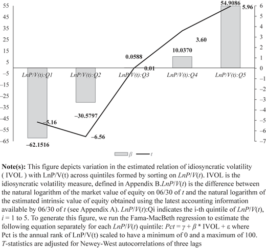
Our hypothesis development builds on the regularity that IVOL and the degree of mispricing are positively related. , the absolute difference between and , measures the degree of mispricing where is the natural logarithm transformation operator, is the market value of equity at time t, and is the intrinsic value of equity at time t. A larger value of means greater mispricing. Because IVOL and the degree of mispricing are positively related, we have where denotes covariance. For overvalued stocks, = while for undervalued stocks, = . Therefore, for overvalued stocks, while for undervalued stocks, . This suggests a testable hypothesis that the greater the proportion of overvalued observations in the sample, the larger the estimated relation between IVOL and .
, the overvaluation likelihood measure, can be taken as the sum of and a value estimation error [8]. We therefore expect to observe that IVOL's estimated relation with is larger for firms in the top quintile than for firms in the bottom quintile, which Figure 2 shows to be the case. To generate Figure 2, we run the Fama and MacBeth (1973) regression to estimate the following equation for each quintile: , where is the annual rank of scaled to have a minimum of 0 and a maximum of 100. Figure 2 shows that IVOL's estimated relation with monotonically increases from −62.1516 (t = −5.16) to 54.9086 (t = 5.96) as the estimation is moved from the bottom quintile to the top one.
Idiosyncratic volatility and mispricing: direct evidence
Idiosyncratic volatility and mispricing: direct evidence
We substitute or for and redo the analysis. We report the results in Figure IA2 of the Internet Appendix. Panel A shows that IVOL's estimated relation with the annual rank of monotonically increases from −50.7943 (t = −7.02) to 48.2048 (t = 5.71) as the computation is moved from the bottom quintile to the top one. Panel B shows that IVOL's estimated relation with the annual rank of monotonically increases from −50.9163 (t = −3.84) to 82.2379 (t = 7.76) as the computation is moved from the bottom quintile to the top one.
Collectively, Figure 2 and Figure IA2 provide direct evidence that idiosyncratic volatility and the degree of mispricing are positively related.
5.2 Sensitivity to research design choices
Research on the relation between idiosyncratic volatility (IVOL) and is characterized by inconsistent findings. IVOL's estimated relation with is inherently unstable, due to the nonlinearity of IVOL's relation with and with . We reason that variation in research design choices across studies may drive the inconsistency by shaping IVOL's estimated relations with and .
We can think of at least two reasons for which research design choices affect IVOL's estimated relations with and . First, a research design choice can change the proportions of ex ante and ex post undervalued and overvalued observations in the sample. Second, it can change the weight of ex ante significantly undervalued observations and ex post significantly overvalued observations in IVOL's estimated relation with due to its effect on the statistical properties of . A well-known regularity of is that it is right-skewed. for the correction of ex ante undervaluation and for the formation of ex post overvaluation can be very large, but for the correction of ex ante overvaluation and for the formation of ex post undervaluation are at most −1. Therefore, large positive returns driving the right-skewness of high likely stem from the correction of ex ante significant undervaluation and the formation of ex post significant overvaluation.
To demonstrate the validity of the second reason, we estimate IVOL's relation with the continuously compounded return (). is the natural logarithm of 1 plus [9]. is expected to be less right-skewed than , since the logarithm transformation reduces the influence of large positive returns on the statistical distribution. We provide the contrast between and in Table IA9 of the Internet Appendix. As expected, is highly right-skewed while is slightly left-skewed. Gauged by the standard deviation and the difference between the 99th and 1st percentiles of their pooled distributions, the variance of is much larger for firms in the bottom quintile than for firms in the top quintile and for firms in the top quintile than for firms in the bottom quintile. This is consistent with the notion that for the correction of ex ante undervaluation and for the formation of ex post overvaluation can be very large but that for the correction of ex ante overvaluation and for the formation of ex post undervaluation are at most −1. In contrast, the variance of is slightly larger for firms in the top quintile than for firms in the bottom quintile and is significantly smaller for firms in the top quintile than for firms in the bottom quintile.
The contrast between and suggests that observations incurring the correction of ex ante significant undervaluation and observations incurring the formation of ex post significant overvaluation are weighted econometrically less in the estimated relation when is the dependent variable than when is the dependent variable. IVOL and are positively related among ex ante undervalued observations and negatively related among ex ante overvalued observations; and IVOL and are positively related among ex post overvalued observations and negatively related among ex post undervalued observations. Therefore, IVOL's overall estimated relation with realized return is expected to be comparatively smaller when is the dependent variable than when is the dependent variable.
We report the results based on in Table 3. For comparison, we also report the results based on . To ensure comparability, we use standardized () and standardized () with a mean of 0 and a standard deviation of 1 as the dependent variables. Table 3 shows that results based on supports the hypothesis. This is not surprising since there is a one-to-one mapping between and . Importantly, Table 3 shows that, consistent with our expectation, IVOL's estimated relation with realized return is comparatively smaller when is the dependent variable than when is the dependent variable. For instance, IVOL's overall estimated relation with is 1.2142 (t = 1.39) while its overall estimated relation with is −4.4337 (t = −4.17). The proportions of ex ante and ex post undervalued and overvalued observations in the sample are the same regardless of whether or is the dependent variable. Therefore, the contrast between and regarding their estimated relations with IVOL is driven by the difference between their statistical properties and the ensuing weight of observations incurring the correction of ex ante significant undervaluation and observations incurring the formation of ex post significant overvaluation in their estimated relation with IVOL.
Raw return vs the continuously compounded return
| Variable | ||||||
|---|---|---|---|---|---|---|
| IVOL (λ1) | 1.2142 (1.39) | −4.4337** (−4.17) | 4.3283** (3.47) | −1.1580 (−0.93) | −2.6969** (−3.95) | −7.1910** (−6.55) |
| IVOL * LnP/V(t):Q2 (λ2) | −3.8638** (−4.56) | −2.8613** (−4.28) | ||||
| IVOL * LnP/V(t):Q3 (λ3) | −4.3886** (−5.22) | −4.1540** (−4.82) | ||||
| IVOL * LnP/V(t):Q4 (λ4) | −5.7958** (−7.66) | −6.3433** (−8.06) | ||||
| IVOL * LnP/V(t):Q5 (λ5) | −7.2149** (−7.65) | −8.4960** (−7.88) | ||||
| IVOL * LnP/V(t + 1):Q2 (λ2) | 2.1056** (3.56) | 2.7174** (3.91) | ||||
| IVOL * LnP/V(t + 1):Q3 (λ3) | 2.4558** (3.64) | 3.0296** (3.85) | ||||
| IVOL * LnP/V(t + 1):Q4 (λ4) | 5.1569** (6.66) | 4.9885** (5.64) | ||||
| IVOL * LnP/V(t + 1):Q5 (λ5) | 16.2895** (7.70) | 11.7653** (5.84) | ||||
| N | 180,717 | 180,717 | 180,717 | 180,717 | 180,717 | 180,717 |
| R2 | 0.1267 | 0.1614 | 0.1306 | 0.1657 | 0.3032 | 0.3670 |
| LnP/V(t):Qi/LnP/V(t + 1):Qi | No | No | Yes | Yes | Yes | Yes |
| Controls | Yes | Yes | Yes | Yes | Yes | Yes |
| Industry FE | Yes | Yes | Yes | Yes | Yes | Yes |
| λ1 + λ2 | 0.4644 (0.31) | −4.0193** (−2.83) | −0.5912 (−0.65) | −4.4736** (−3.44) | ||
| λ1 + λ3 | −0.0603 (−0.04) | −5.3121** (−3.50) | −0.2410 (−0.25) | −4.1614** (−3.08) | ||
| λ1 + λ4 | −1.4676 (−1.01) | −7.5013** (−5.08) | 2.4601* (2.38) | −2.2025 (−1.56) | ||
| λ1 + λ5 | −2.8867† (−1.85) | −9.6541** (−5.85) | 13.5927** (6.11) | 4.5743† (1.99) |
Note(s): This table presents results of the analysis that uses the continuously compounded return as the dependent variable. is stock return over 07/01 of t to 06/30 of t + 1, t = 1966 to 2015. , the continuously compounded return, is the natural logarithm of 1 plus . () is standardized () with a mean of 0 and a standard deviation of 1. is the idiosyncratic volatility measure, defined in Appendix 2. is the difference between the natural logarithm of the market value of equity on 06/30 of t and the natural logarithm of the estimated intrinsic value of equity obtained using the latest accounting information available by 06/30 of t (see Appendix 1). is an indicator variable that equals 1 if is in the i-th quintile (0 otherwise), i = 1 to 5. Industry FE stands for industry fixed effects. Controls stands for control variables and are defined in Appendix 2. T-statistics in parentheses are adjusted for Newey-West autocorrelations of three lags. **, *, and † denote statistical significance at the 1, 5, and 10% levels, respectively, using a 2-tailed test
We next examine the effect of screen for price on IVOL's estimated relation with . Asset pricing studies have generally excluded observations with very low price, arguing that price movements of such observations are susceptible to microstructure biases. However, these studies differ regarding the price threshold for exclusion. Moreover, these studies rarely specify the timing of measuring stock price.
Table IA10 of the Internet Appendix reports results of the analysis that examines the effect of screen for price on the sample composition and on the property of . Panel A shows the effect of screen for the ex ante stock price (Price(t)). Price(t) is stock price on 06/30 of t. As the ex ante price threshold for exclusion increases from $0 to $1 to $5, observations incurring the correction of ex ante significant undervaluation and observations incurring the formation of ex post significant overvaluation are weighted comparatively less and observations incurring the formation of ex post undervaluation are weighted comparatively more in IVOL's estimated relation with . IVOL is positively related to among ex ante undervalued stocks and to among ex post overvalued stocks and negatively related to among ex post undervalued stocks. IVOL's overall estimated relation with is thus expected to decrease with increase in the ex ante price threshold for exclusion.
Panel B of Table IA10 shows the effect of screen for ex post stock price (Price (t + 1)). Price (t + 1) is stock price on 06/30 of t + 1. As the ex post price threshold for exclusion increases from $0 to $1 to $5, observations incurring the correction of ex ante significant undervaluation are weighted comparatively more and observations incurring the formation of ex post undervaluation are weighted comparatively less in IVOL's estimated relation with . IVOL is positively related to among ex ante undervalued observations and negatively related to among ex post undervalued stocks. IVOL's overall estimated relation with is thus expected to increase with increase in the ex post price threshold for exclusion.
Panel C of Table IA10 shows the effect of screen for average stock price (AvgPrice). AvgPrice is the average of Price(t) and Price (t + 1). Panel C shows that the effect of screen for average stock price (AvgPrice) resembles but is weaker than the effect of screen for ex post stock price. IVOL's overall estimated relation with is thus expected to increase with increase in the average price threshold for exclusion but less so than with increase in the ex post price threshold for exclusion.
Table 4 reports results of the analysis that examines the effect of screen for price on IVOL's overall estimated relation with . As expected, with(out) control variables, when the ex ante price threshold for exclusion increases from $0 to $1 to $5, IVOL's overall estimated relation with decreases from 0.8143 (t = 1.39) (0.8626 (t = 0.99)) to 0.2863 (t = 0.48) (0.4196 (t = 0.48)) to −1.1268 (t = −2.08) (−0.6503 (t = −0.73)); when the ex post price threshold for exclusion increases from $0 to $1 to $5, IVOL's overall estimated relation with increases from 0.8143 (t = 1.39) (0.8626 (t = 0.99)) to 2.4014 (t = 3.66) (2.6923 (t = 3.14)) to 7.9500 (t = 8.03) (8.4361 (t = 7.51)); and when the average price threshold for exclusion increases from $0 to $1 to $5, IVOL's overall estimated relation with increases from 0.8143 (t = 1.39) (0.8626 (t = 0.99)) to 1.6416 (t = 2.61) (1.7637 (t = 2.03)) to 4.8574 (t = 5.60) (4.8036 (t = 4.63)).
The effect of screen for price
| Variable | All | Price(t) ≥ $1 | Price(t) ≥ $5 | Price(t + 1) ≥ $1 | Price(t + 1) ≥ $5 | AvgPrice ≥ $1 | AvgPrice ≥ $5 |
|---|---|---|---|---|---|---|---|
| (1) | (2) | (3) | (4) | (5) | (6) | (7) | |
| IVOL | 0.8626 (0.99) | 0.4196 (0.48) | −0.6503 (−0.73) | 2.6923** (3.14) | 8.4361** (7.51) | 1.7637* (2.03) | 4.8036** (4.63) |
| N | 187,231 | 182,634 | 151,208 | 180,911 | 148,786 | 182,721 | 151,693 |
| R2 | 0.0313 | 0.0300 | 0.0331 | 0.0320 | 0.0532 | 0.0319 | 0.0391 |
| Controls | No | No | No | No | No | No | No |
| Industry FE | No | No | No | No | No | No | No |
| IVOL | 0.8143 (1.39) | 0.2863 (0.48) | −1.1268* (−2.08) | 2.4014** (3.66) | 7.9500** (8.03) | 1.6416* (2.61) | 4.8574** (5.60) |
| N | 180,717 | 176,468 | 146,385 | 174,856 | 144,166 | 176,563 | 146,914 |
| R2 | 0.1267 | 0.1290 | 0.1489 | 0.1296 | 0.1688 | 0.1288 | 0.1510 |
| Controls | Yes | Yes | Yes | Yes | Yes | Yes | Yes |
| Industry FE | Yes | Yes | Yes | Yes | Yes | Yes | Yes |
Note(s): This table presents results of the analysis that examines the effect of screen for price on the estimated relation of idiosyncratic volatility (IVOL) with realized return (). Price(t) (Price (t + 1)) is stock price on 06/30 of t (t + 1) and AvgPrice is the average of Price(t) and Price (t + 1). The dependent variable () is stock return over 07/01 of t through 06/30 of t + 1, t = 1966 to 2015. is the idiosyncratic volatility measure, defined in Appendix 2. Industry FE stands for industry fixed effects. Controls stands for control variables, defined in Appendix 2. T-statistics in parentheses are adjusted for Newey-West autocorrelations of three lags. **, *, and † denote statistical significance at the 1, 5, and 10% levels, respectively, using a 2-tailed test
We next examine the effect of screen for size on IVOL's estimated relation with . Asset pricing studies may also exclude small stocks, arguing that data quality of those stocks is low due to their illiquidity and ensuing noise in stock pricing and that their economic significance is trivial. In practice, studies have great discretion over the size threshold for exclusion. Moreover, these studies rarely specify the timing of measuring size.
Table IA11 of the Internet Appendix reports results of the analysis that examines the effect of screen for size on the sample composition and on the property of . As shown in Tables IA10 and IA11, the effect of screen for the ex ante size resembles the effect of screen for the ex ante stock price; the effect of screen for the ex post size resembles the effect of screen for the ex post stock price; and the effect of screen for average size resembles the effect of screen for average stock price. Table 5 shows that as expected IVOL's overall estimated relation with decreases with increase in the ex ante size threshold for exclusion, increases with increase in the ex post size threshold for exclusion, and increases with increase in the average size threshold for exclusion but less than with increase in the ex post size threshold for exclusion.
The effect of screen for size
| Variable | All | SizePct(t) ≥ 10% | SizePct(t) ≥ 30% | SizePct(t + 1) ≥ 10% | SizePct(t + 1) ≥ 30% | AvgSizePct ≥ 10% | AvgSizePct ≥ 30% |
|---|---|---|---|---|---|---|---|
| (1) | (2) | (3) | (4) | (5) | (6) | (7) | |
| IVOL | 0.8626 (0.99) | −0.2976 (−0.33) | −1.1526 (−1.22) | 4.1343** (4.55) | 8.4028** (7.89) | 2.4749** (2.73) | 4.4690** (4.21) |
| N | 187,231 | 168,097 | 130,999 | 168,490 | 131,051 | 168,489 | 131,051 |
| R2 | 0.0313 | 0.0336 | 0.0382 | 0.0373 | 0.0536 | 0.0357 | 0.0429 |
| Controls | No | No | No | No | No | No | No |
| Industry FE | No | No | No | No | No | No | No |
| IVOL | 0.8143 (1.39) | −0.2989 (−0.47) | −1.5151* (−2.03) | 3.6225** (4.75) | 7.4104** (7.26) | 2.2511** (3.17) | 3.9276** (4.07) |
| N | 180,717 | 162,468 | 127,147 | 162,906 | 127,253 | 162,864 | 127,246 |
| R2 | 0.1267 | 0.1412 | 0.1680 | 0.1479 | 0.1859 | 0.1432 | 0.1703 |
| Controls | Yes | Yes | Yes | Yes | Yes | Yes | Yes |
| Industry FE | Yes | Yes | Yes | Yes | Yes | Yes | Yes |
Note(s): This table presents results of the analysis that examines the effect of screen for size on the estimated relation of idiosyncratic volatility (IVOL) with realized return (). SizePct(t) (SizePct (t + 1)) is the annual rank of firm size on 06/30 of t (t + 1). AvgSizePct is the annual rank of the average of firm size on 06/30 of t and firm size on 06/30 of t + 1. SizePct(t), SizePct (t + 1) and AvgSizePct are scaled to have a minimum of 0 and a maximum of 1. is idiosyncratic volatility measure, defined in Appendix 2. Industry FE stands for industry fixed effects. Controls stands for control variables, defined in Appendix 2. T-statistics in parentheses are adjusted for Newey-West autocorrelations of three lags. **, *, and † denote statistical significance at the 1, 5, and 10% levels, respectively, using a 2-tailed test
In practice, a study involves several research design choices. These research design choices can cancel out or reinforce each other's effect on IVOL's estimated relation with depending on the combination of the research design choices, which Table IA12 shows to be the case. It is so far evident that ostensibly immaterial variations in research design choices (e.g. the price and size threshold for exclusion, the timing of measuring price and size, and the weighting scheme) can cause the estimated relation between idiosyncratic volatility and realized return to change dramatically and even switch sign in a predictable manner due to their effects on IVOL's relations with and .
5.3 Potential solutions
IVOL's relations with and cause its estimated relation with to be a potentially biased estimate of its relation with expected return. and are measurement errors of as the proxy for expected return. Portfolio grouping and instrument variables are standard methods for addressing the estimation bias resulting from measurement errors, but neither seems able to remove the bias resulting from IVOL's relations with and . The instrument variable approach requires instrument variables that are correlated with IVOL but not with the degree of mispricing and hence not with and ; such instrumental variables seem extremely difficult – if not impossible – to find.
To apply portfolio grouping, we need to sort observations by IVOL and compute the portfolio average of . If and could cancel out at the portfolio level, portfolio grouping would remove the bias. To explore the effectiveness of portfolio grouping, we apply it to estimate IVOL's relation with . Specifically, we sort observations into five groups independently on IVOL and () each year and then form portfolios at the intersections of IVOL quintiles and () quintiles. Table 6 reports the time-series average of equal-weighted returns for each portfolio. We calculate the time-series average of portfolio returns as in the following regression:
where is portfolio ; is the equal-weighted average of returns over 07/01 of t through 06/30 of t + 1 for firms in portfolio , t = 1966 to 2015; and is the residual. T-statistics are adjusted for Newey-West autocorrelations of three lags.
Idiosyncratic volatility and return: portfolios
| IVOL:Q1 | IVOL:Q2 | IVOL:Q3 | IVOL:Q4 | IVOL:Q5 | Q5-Q1 | |
|---|---|---|---|---|---|---|
| All | 0.1412** (6.23) | 0.1471** (6.16) | 0.1530** (5.51) | 0.1529** (4.93) | 0.1847** (4.98) | 0.0435 (1.33) |
| LnP/V(t):Q1 | 0.1630** (5.46) | 0.1701** (5.80) | 0.1946** (6.31) | 0.2001** (5.70) | 0.2841** (6.22) | 0.1212** (2.80) |
| LnP/V(t):Q2 | 0.1510** (6.44) | 0.1602** (5.89) | 0.1683** (5.49) | 0.1650** (5.18) | 0.1872** (4.80) | 0.0362 (1.18) |
| LnP/V(t):Q3 | 0.1402** (6.65) | 0.1433** (5.80) | 0.1573** (5.42) | 0.1610** (4.90) | 0.1604** (4.46) | 0.0201 (0.66) |
| LnP/V(t):Q4 | 0.1342** (6.21) | 0.1395** (6.59) | 0.1348** (5.14) | 0.1372** (4.41) | 0.1337** (3.67) | −0.0005 (−0.01) |
| LnP/V(t):Q5 | 0.1180** (5.40) | 0.1244** (5.03) | 0.1161** (3.98) | 0.1105** (3.45) | 0.0652† (1.79) | −0.0528 (−1.51) |
| LnP/V(t + 1):Q1 | 0.0167 (0.63) | −0.0211 (−0.79) | −0.0688* (−2.24) | −0.1154** (−3.07) | −0.1209** (−3.47) | −0.1376** (−4.70) |
| LnP/V(t + 1):Q2 | 0.0805** (2.95) | 0.0557* (2.19) | 0.0404 (1.63) | 0.0342 (1.19) | 0.0748* (2.10) | −0.0057 (−0.17) |
| LnP/V(t + 1):Q3 | 0.1339** (4.95) | 0.1372** (5.81) | 0.1311** (4.85) | 0.1422** (5.09) | 0.1959** (5.46) | 0.0620† (1.75) |
| LnP/V(t + 1):Q4 | 0.1853** (6.49) | 0.2041** (7.59) | 0.2306** (7.99) | 0.2464** (7.50) | 0.3428** (8.05) | 0.1575** (3.82) |
| LnP/V(t + 1):Q5 | 0.2341** (7.51) | 0.3052** (10.31) | 0.4151** (10.13) | 0.5069** (8.46) | 0.6955** (8.28) | 0.4614** (5.29) |
Note(s): This table reports the time-series average of equal-weighted returns for portfolios formed by sorting stocks independently on idiosyncratic volatility (IVOL) and the overvaluation likelihood measure (LnP/V). This table also reports the time-series average of equal-weighted returns for portfolios formed by sorting only on IVOL. is the idiosyncratic volatility measure, defined in Appendix 2. indicates the i-th quintile of , i = 1 to 5. is the difference between the natural logarithm of the market value of equity on 06/30 of t and the natural logarithm of the estimated intrinsic value of equity obtained using the latest accounting information available by 06/30 of t, t = 1966 to 2015 (see Appendix 1). indicates the i-th quintile of , i = 1 to 5. The time-series average of portfolio returns is calculated as in the following regression:
where denotes portfolio ; is the equal-weighted average of returns over 07/01 of t through 06/30 of t + 1 for firms in portfolio ; and is the residual. T-statistics in parentheses are adjusted for Newey-West autocorrelations of three lags. **, *, and † denote statistical significance at the 1, 5, and 10% levels, respectively, using a 2-tailed test
Table 6 shows that within each IVOL quintile, decreases monotonically as the computation is moved from the bottom to the top quintile. This is consistent with measuring the ex ante overvaluation likelihood. Importantly, the difference between the top and the bottom IVOL quintiles regarding decreases monotonically from 0.1212 (t = 2.80) to −0.0528 (t = −1.51) as the computation is moved from the bottom to the top quintile. Table 6 also shows that within each IVOL quintile, increases monotonically as the computation is moved from the bottom to the top quintile. This is consistent with measuring the ex post overvaluation likelihood. Importantly, the difference between the top and the bottom IVOL quintiles regarding increases monotonically from −0.1376 (t = −4.70) to 0.4614 (t = 5.29) as the computation is moved from the bottom to the top quintile.
Firms differing in idiosyncratic volatility may also differ in their exposure to traditional risk factors. In the Internet Appendix, we report risk-adjusted returns based on (1) the capital asset-pricing model (CAPM) in Table IA13 and (2) a six-factor model in Table IA14 [10]. As shown in Tables IA13 and IA14, our inference remains the same after controlling for exposure to these standard risk factors.
In summary, the inference drawn using portfolio grouping is the same as the inference drawn using the Fama-MacBeth regression. That is, portfolio grouping cannot address the bias resulting from IVOL's relations with and .
Some studies propose methods for purging of the measurement errors (e.g. Hou & van Dijk, 2019). These methods generally build on Campbell and Shiller's (1988) return decomposition. According to Campbell and Shiller's (1988) return decomposition, can be decomposed into expected return, discount rate news (i.e. shocks to discount rates), and cash flow news (i.e. shocks to expected cash flows). Because the cash-flow-news variance seems to dominate the discount-rate-news variance (Chen, Da, & Zhao, 2013; Vuolteenaho, 2002), these methods focus on purging of cash flow news. Sharing Elton's (1999) concern about the effectiveness of such methods in addressing the measurement errors of , we doubt their effectiveness in addressing the bias resulting from IVOL's covariance with and with for at least two reasons. First, cash flow news and discount rate news seem to capture things other than and . Conceptually, discount rate news and cash flow news are change in investors' expected return and change in investors' expectations of future cash flows, respectively. If rationally determined, they jointly capture change in investors' estimate of the intrinsic value. Second, there is no way to evaluate the effectiveness of such methods because IVOL's s relation with expected return is unknown.
To explore the effectiveness of such methods, we follow Hou and van Dijk (2019) and control for profitability shock (ProfitabilityShock). ProfitabilityShock is the difference between profitability of t + 1 and the expected profitability of t + 1 obtained using Hou and van Dijk's (2019) method. According to Hou and van Dijk (2019), ProfitabilityShock captures the cash flow news. Guided by Campbell and Shiller's (1988) return decomposition, we reason that realized return is also driven by change in the intrinsic value, at least to a large extent. As turned out in this study, the intrinsic value estimate based on Rhodes–Kropf et al. (2005) method exhibits excellent empirical validity regardless of its simplicity. Therefore, we also control for the percentage change (PctChgV) in the estimated intrinsic value of equity from 06/30 of t to 06/30 of t + 1. In our estimation sample, ProfitabilityShock and PctChgV are positively correlated: 0.20 (Pearson) and 0.34 (Spearman). This high positive correlation is consistent with cash flow news reflecting change in investors' estimate of the intrinsic value.
Table 7 presents results of the analysis that controls for ProfitabilityShock and PctChgV. Three results deserve attention. First, both ProfitabilityShock and PctChgV are, as expected, positively related to . Second, as gauged by the magnitude of T-statistics, PctChgV turns out to be the most significant determinant of among all explanatory variables. Third, controlling for ProfitabilityShock and PctChgV has no material impact on our inference, suggesting that these proposed methods cannot address the bias resulting from IVOL's covariance with and with .
Controlling for profitability shocks and percentage change in the estimated intrinsic value
| Variable | (1) | (2) | Variable | (3) |
|---|---|---|---|---|
| IVOL (λ1) | 1.8839** (2.77) | 4.0718** (4.66) | IVOL (λ1) | −0.9180† (−1.78) |
| IVOL * LnP/V(t):Q2 (λ2) | −2.7312** (−6.02) | IVOL * LnP/V(t + 1):Q2 (λ2) | 0.8882* (2.40) | |
| IVOL * LnP/V(t):Q3 (λ3) | −3.3453** (−5.93) | IVOL * LnP/V(t + 1):Q3 (λ3) | 1.3149* (2.66) | |
| IVOL * LnP/V(t):Q4 (λ4) | −3.8323** (−6.33) | IVOL * LnP/V(t + 1):Q4 (λ4) | 3.3996** (4.38) | |
| IVOL * LnP/V(t):Q5 (λ5) | −5.4185** (−8.35) | IVOL * LnP/V(t + 1):Q5 (λ5) | 12.0283** (9.48) | |
| ProfitabilityShock | 1.5800** (4.16) | 1.5210** (4.23) | ProfitabilityShock | 1.5355** (3.84) |
| PctChgV | 0.1147** (13.24) | 0.1430** (13.92) | PctChgV | 0.2148** (16.88) |
| N | 177,682 | 177,682 | N | 177,682 |
| R2 | 0.1896 | 0.1982 | R2 | 0.4043 |
| LnP/V(t):Qi | No | Yes | LnP/V(t + 1):Qi | Yes |
| Controls | Yes | Yes | Controls | Yes |
| Industry FE | Yes | Yes | Industry FE | Yes |
Note(s): This table presents results of the analysis that controls for profitability shocks and percentage change in the estimated intrinsic value of equity from 06/30 of t to 06/30 of t + 1. ProfitabilityShock is the difference between profitability of t + 1 and the expected profitability of t + 1 obtained using the method introduced in Hou and van Dijk (2019). PctChgV is the percentage change in the estimated intrinsic value of equity from 06/30 of t to 06/30 of t + 1. The dependent variable () is stock return over 07/01 of t to 06/30 of t + 1, t = 1966 to 2015. is the idiosyncratic volatility measure, defined in Appendix 2. is the difference between the natural logarithm of the market value of equity on 06/30 of t and the natural logarithm of the estimated intrinsic value of equity obtained using the latest accounting information available by 06/30 of t, t = 1966 to 2015 (see Appendix 1). is an indicator variable that equals 1 if is in the i-th quintile (0 otherwise), i = 1 to 5. T-statistics in parentheses are adjusted for Newey-West autocorrelations of three lags. **, *, and † denote statistical significance at the 1, 5, and 10% levels, respectively, using a 2-tailed test
Two forms of wishful thinking in addressing the bias are still possible. One is thinking that increasing the sample size may “diversify” away the bias. The other is thinking that one can construct a sample in which firms are properly priced and, as a result, the bias resulting from IVOL's covariance with and with can be ignored. Empirically, it is always possible that the bias may accidentally cancel out, even without a large sample, and that it may be negligible, even without a specially constructed sample. However, because IVOL's relation with expected return is unknown, there is no way to know whether such bias has cancelled out even if it has or to know whether such bias is negligible even if it is (Black, 1986).
In sum, it seems that existing methods cannot address the bias resulting from the covariance of idiosyncratic volatility (IVOL) with the mispricing-correction component () and the mispricing-formation component () of realized return ().
6. Conclusion
Idiosyncratic volatility (IVOL) has a dual effect on stock pricing: It affects stock pricing through its effect on both investors' expected return and stock pricing efficiency. Stock pricing efficiency, on average, is low for firms with high IVOL because high IVOL is associated with high arbitrage risks. That is, the extent to which stock price deviates from its underlying equity value is larger for firms with higher IVOL. Due to its dual effect on stock pricing, IVOL's estimated relation with realized return () captures its relations with both expected return and the mispricing-related component (the ex ante mispricing correction component () and the ex post mispricing formation component ()). IVOL is positively related to among ex ante undervalued stocks and negatively related to among ex ante overvalued stocks; IVOL is negatively related to among ex post undervalued stocks and positively related to among ex post overvalued stocks.
We find that IVOL's estimated relation with decreases and switches sign from positive to negative as the estimation sample consists of proportionately more ex ante overvalued observations and that it increases and switches sign from negative to positive as the estimation sample consists of proportionately more ex post overvalued observations. Our finding suggests that IVOL's relations with and dominate its relation with expected return in its estimated relation with . One thus cannot infer the sign – let alone the magnitude – of IVOL's relation with expected return from its estimated relation with . Moreover, we show that existing methods cannot address the bias resulting from IVOL's relation with and with . We further show that ostensibly immaterial variations in oft-employed research design choices can cause IVOL's estimated relation with to vary dramatically and even switch sign as a result of their effects on IVOL's estimated relations with and .
Our study contributes to research on the relation between idiosyncratic volatility (IVOL) and realized return () by shedding light on the inconsistent and puzzling results about the relation. Our findings suggest that we cannot draw any reliable inference about the sign of IVOL's relation with expected return from its estimated relation with . Therefore, the negative estimated relation of idiosyncratic volatility with realized return documented in some studies does not necessarily contradict the prediction of classic asset pricing theories. That is, this documented negative relation may not be an asset pricing puzzle. Our study also shows that IVOL's estimated relation with realized return varies with research design choices due to their effects on its relation with the mispricing-related components, suggesting that the inconsistency of the results about IVOL's estimated relation with stems from variations in research design choices across studies. In summary, our study shows that the confusion about the relation of idiosyncratic volatility with realized return stems from neglecting its effect on stock pricing efficiency in research designs and results interpretation.
The authors thank workshop participants at the Hong Kong Polytechnic University and Peking University. The current version of this working paper benefits from conversations with Tarun Chordia and John Wei.
Notes
We choose not to provide a comprehensive literature review. Readers can refer to Hou and Loh (2016) for their excellent survey of research about the relation between idiosyncratic volatility and realized return.
PriceDelay = 1 – (R2 of the restricted model/R2 of the non-restricted model), where the non-restricted model is specified as , ri,l is return on stock i in week l, Rm,l is return for the CRSP value-weighted market index in week l, and the restricted model constrains .
“It [Noise] keeps us from knowing the expected return on a stock or portfolio … We might define an efficient market as one in which price is within a factor of 2 of value, i.e. the price is more than half of value and less than twice value. The factor of 2 is arbitrary, of course. Intuitively, though, it seems reasonable to me, in the light of sources of uncertainty about value and the strength of the forces tending to cause price to return to value. By this definition, I think almost all markets are efficient almost all of the time. ‘Almost all’ means at least 90%” Black (1986, pp. 529, 533).
Fisher Black joined Goldman Sachs in 1984 and worked there until his death in 1995 (https://en.wikipedia.org/wiki/Fischer_Black).
For brevity, we do not report descriptive statistics of variables for samples used in other tests; they will be provided on request.
For brevity, Table 2 does not report coefficient estimates for control variables; we report these in Table IA1 of the Internet Appendix. Table IA1 shows that the sign of statistically significant coefficient estimates is consistent with that reported in prior studies when the model specification ignores that IVOL's estimated relation with varies with the proportion of ex ante (expost) overvalued observations in the sample. For instance, is negatively related to firm size (Size), net stock issues (NetStkIssue), positive accruals (PosTtlAcc), and asset growth (AssetGrowth), and positively related to the book-to-market ratio (B/M) and profitability (PosIB/BE).
We choose not to use analysts' earnings-per-share (EPS) forecasts from I/B/E/S because the model-based approach allows us a broader sample in terms of both time periods and firms covered.
, where is the natural logarithm transformation operator, is the market value, is the intrinsic value, and is the estimated intrinsic value.
We assign −0.999 to firms whose is −1.
The six factors are the small-minus-big (SMB) factor, the high-minus-low (HML) factor, the momentum (MOM) factor, the robust-minus-weak (RMW) factor, the conservative-minus-aggressive (CMA) factor and the market factor.
The percentage of observations encountering the short selling of their common shares is lower for the top quintile than for the fourth quintile, possibly because firms in the top quintile are more likely to aggressively fight short arbitrageurs and/or because shareholders of these firms are less willing to lend their shares, since they can benefit more from selling highly overvalued stocks than from collecting lending fees (Lamont, 2012).
References
Appendix 1 The equity overvaluation likelihood measure
The overvaluation likelihood measure (LnP/V) is the difference between the natural logarithm of the market value of equity and the natural logarithm of the estimated intrinsic value of equity. We adopt Rhodes–Kropf et al. (2005) method to estimate the intrinsic value of equity. We use LnP/V as our primary measure of overvaluation likelihood.
Rhodes–Kropf et al. (2005) method takes the intrinsic value of equity as a function of accounting items. The details of their method are as follows. First, we estimate the following equation separately for each of Fama-French's 12 industry groups each year:
where i is firm i; t is fiscal year t; j is industry j; is the natural logarithm of market value of equity; is the natural logarithm of book value of equity; is the natural logarithm of the absolute value of net income; is an indicator variable that equals 1 if net income is negative (0 otherwise); and LEV is the book leverage (that is, the ratio of total liabilities to total assets). All variables are measured at the end of fiscal year t. The sample period is 1950–2015. Untabulated results show that the R2 ranges from 64.96 to 98.33%, indicating that the accounting items in Equation (A.1) explain most within-industry variance in firm-level market value at a given time.
Second, we compute the rolling average of to obtain . Our use of the rolling average avoids look-forward bias. We start the computation in 1966 to ensure the reliability of . Following Rhodes–Kropf et al. (2005), we compute the estimated intrinsic value of equity (log) (LnV) as
and use the difference between the natural logarithm of the market value of equity () and the natural logarithm of the estimated intrinsic value of equity (log) () to gauge the relative overvaluation likelihood.
Prior studies provide initial evidence about the validity of for gauging the relative overvaluation likelihood. Rhodes–Kropf et al. (2005) show that the pattern of merger and acquisition activities varies with as theoretically predicted; Chi and Gupta (2009) find that is positively related to subsequent income-increasing earnings management, which is consistent with Jensen's (2005) prediction that equity overvaluation induces managers to inflate reported earnings to sustain the overvaluation. If , as a measure of the relative overvaluation likelihood at the fiscal year-end of t, has adequate validity, we expect that firms with larger , than firms with smaller , will (1) deliver higher returns in fiscal year t and lower returns in fiscal year t + 1 (Frankel & Lee, 1998); (2) encounter higher percentages of outstanding common shares shorted at the fiscal year-end of t, since short arbitrageurs are expected to target overvalued stocks (Karpoff & Lou, 2010); (3) make more stock issues in fiscal year t + 1 because firms tend to issue stocks when their stocks are overvalued (Baker & Wurgler, 2002); and (4) generate higher percentages of sales from acquisitions in fiscal year t + 1 because overvalued firms are more likely than undervalued firms to engage in acquisitions (Rhodes–Kropf et al., 2005).
To compare observations with larger and smaller , we sort observations into five equal groups according to . Table A1 presents the comparison results. Rt is stock return over the 12-month period of fiscal year t and Rt + 1 is stock return over the 12-month period of fiscal year t + 1. Table A1 shows that when the computation is moved from the bottom to the top quintile, Rt increases monotonically and Rt + 1 decreases monotonically. Shortt (short interests) is the percentage of outstanding common shares shorted at the end of fiscal year t; NetStkIssuet + 1 (net stock issues) is change in the natural logarithm of split-adjusted shares outstanding from the end of fiscal year t to the end of fiscal year t + 1; SalesByACQt + 1 (sales contributed by acquisitions) is the percentage of sales arising from acquisitions in fiscal year t + 1. Table A1 shows that (1) Shortt and SalesByACQt + 1 increase monotonically from the bottom to the top quintile; (2) NetStkIssuet + 1 first decreases and then increases monotonically; (3) observations in the top quintile make significantly more net stock issues than those in the bottom quintile in fiscal year t + 1; (4) the percentage of observations with positive net stock issues or with nonzero sales from acquisitions or with more than 20% sales from acquisitions in fiscal year t + 1 increases monotonically from the bottom to the top quintile; and (5) the percentage of observations encountering the short selling of their common shares at the end of fiscal year t is much higher for the top quintile than for the bottom quintile [11]. Together with the findings of Rhodes–Kropf et al. (2005) and Chi and Gupta (2009), these comparison results suggest that well captures the relative overvaluation likelihood of observations. That is, observations with larger are more likely to be overvalued than those with smaller .
Validity of LnP/V as the overvaluation likelihood measure
| Variable | LnP/V:Q1 | LnP/V:Q2 | LnP/V:Q3 | LnP/V:Q4 | LnP/V:Q5 | Q5 - Q1 | ||||||
|---|---|---|---|---|---|---|---|---|---|---|---|---|
| N | Mean | N | Mean | N | Mean | N | Mean | N | Mean | Diff | t | |
| Rt | 49,244 | −10.52% | 49,244 | 4.51% | 49,244 | 12.16% | 49,244 | 21.35% | 49,244 | 39.67% | 50.19% | 120.00 |
| Rt + 1 | 46,259 | 31.15% | 46,259 | 18.91% | 46,259 | 13.90% | 46,259 | 9.58% | 46,259 | 4.58% | −26.57% | −42.24 |
| Shortt | 46,391 | 0.43% | 46,392 | 0.75% | 46,392 | 1.12% | 46,392 | 1.49% | 46,392 | 1.82% | 1.38% | 78.37 |
| % (Shortt > 0) | 46,391 | 24.63% | 46,392 | 38.25% | 46,392 | 48.36% | 46,392 | 55.07% | 46,392 | 52.01% | 27.38% | 89.39 |
| NetStkIssuet + 1 | 46,384 | 4.32% | 46,385 | 3.06% | 46,385 | 3.62% | 46,385 | 4.55% | 46,385 | 7.18% | 2.86% | 25.09 |
| % (NetStkIssuet + 1 > 0) | 46,384 | 52.38% | 46,385 | 59.08% | 46,385 | 64.67% | 46,385 | 69.12% | 46,385 | 76.75% | 24.37% | 80.23 |
| SalesByACQt + 1 | 43,605 | 0.91% | 43,606 | 1.33% | 43,606 | 1.58% | 43,606 | 1.98% | 43,606 | 2.60% | 1.69% | 33.87 |
| % (SalesByACQt + 1 > 0) | 46,384 | 4.26% | 46,385 | 6.67% | 46,385 | 8.11% | 46,385 | 9.99% | 46,385 | 12.65% | 8.39% | 45.05 |
| %(SalesByACQt + 1 > 0.2) | 43,605 | 1.86% | 43,606 | 2.69% | 43,606 | 3.18% | 43,606 | 4.05% | 43,606 | 5.38% | 3.52% | 27.91 |
Note(s): This table presents comparisons between different groups along dimensions that prior studies find vary with equity overvaluation. is the difference between the natural logarithm of the market value of equity at the end of fiscal year t and the natural logarithm of the estimated intrinsic value of equity obtained using accounting information from financial statements of fiscal year t; indicates the i-th quintile of , i = 1 to 5; Rt (Rt + 1) is stock return over the 12-month period of fiscal year t (t + 1); Shortt is the percentage of outstanding common shares shorted at the fiscal year-end of t; NetStkIssuet + 1 is change in the natural logarithm of split-adjusted shares outstanding from fiscal year t to fiscal year t + 1; and SalesByACQt + 1 is the percentage of sales arising from acquisitions in t + 1
Appendix 2
Variable definitionsa
| Variables used in the main test | |
|---|---|
| AssetGrowth | Change in the natural logarithm of assets per split-adjusted share |
| Beta-CMA | Factor loadingb on the conservative-minus-aggressive factor |
| Beta-HML | Factor loading on the high-minus-low factor |
| Beta-MktRf | Factor loading on the market factor |
| Beta-MOM | Factor loading on the momentum factor |
| Beta-RMW | Factor loading on the robust-minus-weak factor |
| Beta-SMB | Factor loading on the small-minus-big factor |
| IB/BE (profitability) | Income before extraordinary items divided by book equity at the beginning of the year |
| IVOL (idiosyncratic volatility) | Standard deviation of residuals from a regression that takes daily excess returns as a function of daily excess market returns and daily returns to the small-minus-big, high-minus-low, momentum, robust-minus-weak, and conservative-minus-aggressive factors |
| B/M | Natural logarithm of the ratio of the book value of equity to the market value of equity |
| LnP/V(t) (overvaluation likelihood) | Difference between the natural logarithm of the market value of equity on 06/30 of t and the natural logarithm of the estimated intrinsic value of equity obtained using the latest accounting information available by 06/30 of t. Estimation details are in Appendix 1 |
| LnP/V(t):Qi | An indicator variable that equals 1 if LnP/V(t) is in the i-th annual quintile (0 otherwise), i = 1 to 5 |
| Momentum | Stock return over the 11-month period ending on 05/31 of t |
| NegIB (loss) | An indicator variable that equals 1 if income before extraordinary items is negative (0 otherwise) |
| NetStkIssue (net stock issues) | Change in the natural logarithm of split-adjusted shares outstanding from 06/30 of t − 1 to 06/30 of t |
| NegTtlAcc (negative total accruals) | TtlAcc for firms with negative accruals (0 otherwise) |
| PosIB/BE (positive profitability) | IB/BE for firms with positive IB/BE (0 otherwise) |
| PosTtlAcc (positive total accruals) | TtlAcc for firms with positive accruals (0 otherwise) |
| Stock return over 07/01 of t to 06/30 of t + 1, t = 1966 to 2015 | |
| Size | Natural logarithm of the market value of equity on 06/30 of t |
| TtlAcc (total accruals) | Change in operating working capital per split-adjusted share divided by total assets per split-adjusted share |
| ZeroNetStkIssue | An indicator variable that equals 1 if NetStkIssue equals 0 (0 otherwise) |
| Other variables | |
| AbsAutoCorr | Absolute value of the first-order autocorrelation of daily returns, computed using data from 07/01 of t − 1 to 06/30 of t |
| AvgPrice | Average of Price(t) and Price(t + 1) |
| AvgSizePct | Annual rank of the average of firm size on 06/30 of t and firm size on 06/30 of t + 1, scaled to have a minimum of 0 and a maximum of 1 |
| Annualized return to the conservative-minus-aggressive (CMA) factor over 07/01 of t to 06/30 of t + 1 | |
| Annualized return to the high-minus-low (HML) factor over 07/01 of t to 06/30 of t + 1 | |
| IVOL3MON | Standard deviation of residuals from a regression that takes daily excess returns as a function of daily excess market returns and daily returns to the small-minus-big, high-minus-low, momentum, robust-minus-weak, and conservative-minus-aggressive factors, computed using daily data from 04/01 of t through 06/30 of t |
| IVOL5Year | Standard deviation of residuals from a regression that takes monthly excess returns as a function of monthly excess market returns and monthly returns to the small-minus-big, high-minus-low, momentum, robust-minus-weak, and conservative-minus-aggressive factors, computed using monthly data from 07/01 of t − 5 through 06/30 of t with at least 12 observations |
| The i-th quintile of , i = 1 to 5 | |
| (continuously compounded return) | Natural logarithm of 1 plus , where is stock return over 07/01 of t to 06/30 of t + 1 |
| Annualized return to the momentum (MOM) factor over 07/01 of t to 06/30 of t + 1 | |
| MTB(t) (market-to-book) | Ratio of the market value of equity on 06/30 of t to the latest book value of equity available by 06/30 of t |
| MTB(t):Qi | An indicator variable that equals 1 if MTB(t) is in the ith annual quintile (0 otherwise), i = 1 to 5 |
| P/V-F&L(t) (the price-to-value ratio) | Ratio of the market value of equity on 06/30 of t to the estimated intrinsic value of equity (V-F&L) that is obtained by incorporating model-based earnings predictions and the industry-specific cost of equity into the empirically tractable version of the residual income valuation model introduced in Frankel and Lee (1998). We adopt Hou, van Dijk, and Zhang's (2012) model-based approach to forecasting earnings and apply Fama and French's (1993) three-factor model to estimate the industry-specific cost of equity |
| P/V-F&L(t):Qi | An indicator variable that equals 1 if P/V-F&L(t) is in the ith annual quintile (0 otherwise), i = 1 to 5 |
| PctChgV | Percentage change in the estimated intrinsic value of equity from 06/30 of t to 06/30 of t + 1 |
| Price(t) (ex ante stock price) | Stock price on 06/30 of t |
| Price(t + 1) (ex post stock price) | Stock price on 06/30 of t + 1 |
| PriceDelay | 1 - (R2 of the restricted model/R2 of the non-restricted model), where the non-restricted model is specified as , ri,l is the return on stock i in week l, Rm,l is the return for the CRSP value-weighted market index in week l, and the restricted model constrains |
| ProfitabilityShock | Difference between profitability of t + 1 and the expected profitability of t + 1 obtained using the method introduced in Hou and van Dijk (2019) |
| Annualized one-month T-bill rate over 07/01 of t to 06/30 of t + 1 | |
| Annualized return on the market portfolio over 07/01 of t to 06/30 of t + 1 | |
| RetSkewness | Return skewness computed using daily return data from 04/01 of t to 06/30 of t |
| (risk-adjusted return) | Computed as where is firm ; is the stock return over 07/01 of t through 06/30 of t + 1 for firm ; is the annualized one-month T-bill rate over the same period; is the annualized return on the market portfolio over the same period; / / / / is the annualized return to the small-minus-big/high-minus-low/momentum/robust-minus-weak/conservative-minus-aggressive factor over the same period; , , , , , and are factor loadings obtained using daily return data from 07/01 of t through 06/30 of t + 1 |
| Annualized return to the robust-minus-weak (RMW) factor over 07/01 of t to 06/30 of t + 1 | |
| SizePct(t) | Annual rank of firm size on 06/30 of t, scaled to have a minimum of 0 and a maximum of 1 |
| SizePct(t + 1) | Annual rank of firm size on 06/30 of t + 1, scaled to have a minimum of 0 and a maximum of 1 |
| Annualized return to the small-minus-big (SMB) factor over 07/01 of t to 06/30 of t + 1 | |
| Standardized with a mean of 0 and a standard deviation of 1 | |
| Standardized with a mean of 0 and a standard deviation of 1 | |
| StkLiq (stock liquidity) | −1 x the natural logarithm of Abdi and Ranaldo's (2017) effective bid-ask spread estimate, computed using daily close, high, and low prices from 07/01 of t − 1 to 06/30 of t |
Note(s): aUnless stated otherwise, all variables are computed using the latest accounting and market information available by 06/30 of t
bThese factor loadings and IVOL are computed using daily data from 07/01 of t − 1 to 06/30 of t, t = 1966 to 2015
Appendix 3
Internet appendix are available in online for this article.

