Evaluation of a control-oriented single-phase transformer core model

A major challenge of modelling inductive transformers is capturing the dynamics of the ferromagnetic core, which includes material-specific effects like saturation, hysteresis, and eddy current losses. According to Mörée and Leijon (2023), the two primary approaches for modelling ferromagnetic hysteresis are Duhem-type and Preisach-based models.

Duhem-type models use an ordinary differential equation (ODE), with the Jiles–Atherton model being a prominent implementation (Jiles and Atherton, 1986). However, evaluating the Jiles–Atherton equations in the presence of measurement noise poses significant numerical challenges.

Preisach-based hysteresis models (Preisach, 1935) approximate the behaviour of ferromagnetic materials through the superposition of numerous independent hysteresis elements. In general, Preisach-based models need an extensive amount of parameters, making their identification challenging. Thus, it is often regarded as a data-driven approach.

A different approach modelling the hysteresis of ferromagnetic materials is the so-called dynamic hysteresis model. It is introduced in Zirka et al. (2014) and is based on the reconstruction of first-order reversal curves. As it describes the behaviour of the hysteresis with the magnetic flux density as the input and the magnetic field strength as the output, the model is particularly useful implementation in circuit simulators and transient simulation (Zirka et al., 2015). The model has been successfully applied to simulate the ferromagnetic losses of a laminated core under PWM excitation in Simulink (Rasilo et al., 2019). This model is considered to be an “equation-free” model. It is implemented as an algorithm instead of equations – which makes the model inconvenient to be applied for control tasks.

Model-based controller design methods often benefit from using models in state-space representation (Khalil, 2014). However, neither the Duhem-type model nor the Preisach model can be expressed in this format, highlighting the need for control-oriented models.

A hysteresis model which can be formulated in a state-space form is the Chua–Stromsmoe model (Chua and Stromsmoe, 1970). An implementation of this approach is described in Ranta et al. (2011). The model is constructed by finding two functions describing the mid-curve and the width of a measured hysteresis loop. Thus, the Chua–Stromsmoe hysteresis model is only applicable for the input waveform that was used to generate the measurement and identifying the model.

In Schwartze et al. (2025a, 2025b), a control-oriented model is introduced which combines both advantages: it can be written in a state-space representation and is valid for arbitrary input signal forms. This model lays the basis for the present paper, which focuses on a more empirical investigation of the control-oriented model with practical applications in mind. The main contributions are as follows:

• A data analysis based on a clustering approach for identifying fundamentally different transformers for a comprehensive model validation.

• The experimental model validation based on the previously chosen transformers exhibiting distinct characteristics.

• A runtime experiment comparing the computational effort between the control-oriented model and the Jiles–Atherton model.

• An investigation concerning the numerical stability of the simulations.

In Section 2, an overview of the control-oriented model described in Schwartze et al. ( 2025b) is given. To validate the mathematical model on a wide range of possible dynamics while minimizing the testing effort, a data analysis is performed in Section 3 and Section 4. In Section 5, the control-oriented model and a model based on the Jiles–Atherton equations are compared to measurements. A performance analysis regarding the computational effort of both models is conducted in Section 6. A conclusion is given in Section 7.

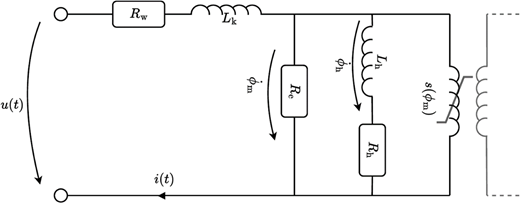
This section gives an overview of the mathematical model derived in Schwartze et al. ( 2025b). The proposed control-oriented model describes one side of a single-phase transformer (i.e. either the primary or the secondary side). This configuration is especially important for model-based testing of transformers, which is the motivation and application considered in this article. It is assumed that a voltage $u$ acts as the input to the system and the output current $i$⁠, on the same side, is regarded as the output of the system. Thus, the model reproduces the dynamics of the inductance seen from one side of the transformer. The corresponding equivalent circuit diagram is depicted in Figure 1.

As the spatial resolution of the relevant field quantities is not important in this context of model-based controller design, a lumped element interpretation can be used.

The proposed control-oriented model consists of three coupled nonlinear ODE, which can be represented in a state-space form (Khalil, 2014) denoted by the following:

where $u$ is the scalar input, $y$ is the scalar output and $x$ represents the state vector:

of the system.

According to the electrical equivalent diagram presented in Figure 1, the states can be interpreted in a physically meaningful way. The first state $x1= ϕm$ denotes the magnetic flux that is present in the ferromagnetic core at any given time instance. The second state $x2= ϕh$ represents a part of this flux, that is responsible for the width of the hysteresis. The output current that flows through the coil is $x3=i$⁠.

As derived in Schwartze et al. ( 2025b), the right-hand side $fx,u$ of the ODE presented in (1a), is as follows:

where $Rw, Lk, Re, Rh, Lh∈ R+$ denote the model parameter. Each of these parameters belong to a corresponding physical effect. The ohmic resistance of the transformer windings is represented by $Rw$⁠. A common approach to model the leakage flux, i.e. magnetic flux that is induced by the coil but not applied to the ferromagnetic material, is to include a leakage inductance $Lk$ in series to the main coil. A constant core-loss resistor $Re$ is used to represent the eddy current losses in the ferromagnetic core. The combination of $Rw$ and $Lh$ is assumed to capture the material-specific hysteresis losses. For a more detailed theoretical analysis, see Schwartze et al. ( 2025b).

As the magnetic flux increases, the ferromagnetic material saturates, which is captured by the function $sx1$⁠. Theoretically, any appropriate function that best describes the saturation characteristic of the ferromagnetic material can be used, a comprehensive overview is given in Fischer and Moser (1956). The function:

presented in Ranta et al. (2011) is found to give an reasonable trade-off between complexity and adaptability to a wide range of different magnetic materials. The positive parameters $β, S, Lm∈ R+$ can be selected to adjust the saturation characteristic. Thus, the proposed model (1) consists of 8 constant parameters, which can be identified through a combination of measurements and optimization, which is explained in more detail in Schwartze et al. ( 2025b).

The characteristics of transformers can be very diverse, depending on their shape, size, ferromagnetic core material and application. To validate the model across a broad range of devices, a data set comprising measurements from 2,000 current transformers (CTs) is analysed.

A standard method for evaluating the operation and accuracy class of CTs is the model-based test (Jäger et al., 2014). A device capable of performing such a test is the CT Analyzer (OMICRON electronics GmbH, 2022). During this test, characteristics of the connected CT are identified. Some important parameters are as follows:

• unsaturated inductance $Lm$⁠: inductance of the CT below the saturation of the material;

• saturation flux $ϕm,s$⁠: material-specific limit for magnetic flux that can be present in the core;

• remanence factor $Kr$⁠: ratio of remanence flux to saturation flux;

• winding resistance $Rw$⁠: ohmic resistance of the windings in the coil; and

• eddy current resistor $Re$⁠: constant core resistor representing the power losses due to the eddy currents induced in the ferromagnetic core.

These parameters are identified purely based on measurements and there is no need for any user input during the procedure. Further, they are connected to physical quantities of the CT such as shape, size and ferromagnetic material. These parameters are assumed to uniquely describe a CT and are therefore selected to form the feature-space for the clustering algorithm.

To identify groups, i.e. clusters, of CTs within the data set, an unsupervised clustering algorithm is used. As described in (Xu and Tian, 2015), selecting a suitable clustering algorithm is not trivial and strongly depends on the data set and the problem at hand. It can be observed that the data points are spread out continuously through the search space which leads to the assumption that the underlying clusters might be convex sets. The present data set is large with a smaller dimensional search space. For this clustering problem, the K-means algorithm (Thorndike, 1953) is an appropriate choice (Xu and Tian, 2015). The K-means algorithm is a well-established method that is computational efficient compared to other clustering algorithms. This property allows multiple reinitializations of the clustering process with reasonable time consumption. The K-means algorithm partitions the data set into $k$ distinct clusters through an iterative process. The data points are assigned to the nearest cluster centroid. In a second step the centroids are updated based on the mean of the assigned points. This process continues until convergence is achieved. For this analysis, the scikit-learn implementation of the K-means algorithm (Pedregosa et al., 2011) is used in Python 3.8.13. The quality of the clustering heavily depends on the initialization of the starting values selected in the first iteration, here the “k-means++” initialization method is used. The algorithm is reevaluated with different starting points for 1,000 times, before the best clustering result is accepted.

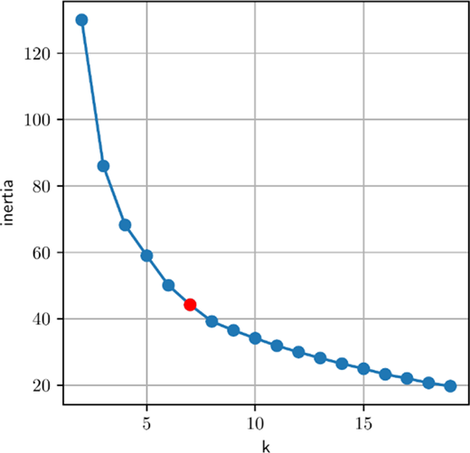
The K-means algorithm needs to know the expected number of clusters $k$a priori. Different methods for selecting the $k$ parameter are described and compared in Yuan and Yang (2019). A simple, yet powerful method is the “elbow-method”. There, the sum of the inertia of all clusters is calculated by the following:

where $nj$ denotes the number of CT measurements per cluster $j$⁠. The variable $dj,i$ represents the $ith$ data point belonging to the $jth$ cluster with the centroid $μj$⁠. This value $J$ is calculated for clustering results with varying values $k$⁠, which leads to the elbow plot depicted in Figure 2. The elbow-method is a visual approach, with the goal of choosing an appropriate number of clusters $k$ that gives a good clustering result (i.e. a small value for $J$⁠) while at the same time preventing over-fitting. The elbow-method is also criticized for being a subjective measure, as no formal definition of the “elbow-point” exists. Therefore, no statement about the optimality for the value of $k$ can be drawn from this method. A detailed analysis of the elbow-method and other alternative approaches is discussed in Schubert (2023). While the elbow-method can be criticized, it is frequently utilized because of its intuitive simplicity and demonstrated effectiveness in practical applications. According to Figure 2, $k=7$ is selected for the considered data set. This marks the first point where the inertia starts to decrease approximately linearly with increasing number of clusters $k$⁠.

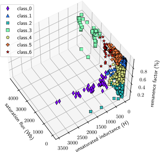
A subspace of the full feature-space depicting the clusters is shown in Figure 3. It is demonstrated that the data set can be visually separated in the feature-space consisting of saturation flux $ϕm,s$⁠, unsaturated inductance $Lm$ and remanence factor $Kr$⁠. This analysis allows to assign some characteristics to each identified group. It is assumed that by verifying the model for the centroid of the cluster, the model will work reasonably well to describe all CTs within this cluster. Three representative CTs of the clusters $C0$⁠, $C2$ and $C3$ are selected for the comparison presented in Section 5 and are described in more detail in Table 1.

The model’s performance is assessed by comparing measurement and simulation over one period, where the voltage $u$ is supplied as an input and the output current $i$ is measured.

Before the control-oriented model can be simulated, its parameters need to be identified during a separate step. This is done based on a combination of direct measurements for the parameters:

• winding resistance $Rw$⁠;

• eddy current losses $Re$⁠; and

• leakage inductance $Lk$⁠.

and an optimization procedure for the parameters:

• hysteresis losses $Rh$ and $Lh$⁠; and

• saturation characteristic $sϕm$⁠.

The identified parameters of the control-oriented model for the CTs from the clusters $C0$⁠, $C2$ and $C3$ are provided in Table 2.

The control-oriented model is also compared to the well-established Jiles–Atherton model, which acts as a baseline and is described in more detail in Albert et al. (2024) and consists of 11 parameters. The ohmic resistance of the windings on the secondary side is reflected in the parameter $Rsec$⁠. The parameters $L12σ$ and $R12σ$ describe the leakage flux between the primary and the secondary side. The geometry of the transformer is modelled by the parameters $Ac$⁠, i.e. the cross-sectional area, and $LFe$⁠, the length of the ferromagnetic core. $RFe$ describes the eddy current losses and corresponds to $Re$ of the control-oriented model. All other parameters are the standard parameters of the Jiles–Atherton model where $Ms$ is the magnetization saturation, $a$ the domain wall density, $α$ the interdomain coupling, $k$ the pinning force and $c$ the magnetization reversibility. The identified parameters of the Jiles–Atherton model are shown in Table 3. For a fair comparison, both, the control-oriented model and the Jiles–Atherton model, are implemented in MATLAB/Simulink 2023a (The MathWorks Inc, 2023a).

To show the general applicability of the control-oriented model, the experiment is performed over a wide range of different input voltage settings $uo$⁠. Here, $o∈1,2,3,4,5,6$ denotes the operation point:

• $u1=58$ V square wave at 50 Hz;

• $u2=56$ V sine wave at 53 Hz;

• $u3=8.75$ V square wave at 50 Hz;

• $u4=14$ V square wave at 50 Hz;

• $u5=118$ V square wave at 5.6 Hz; and

• $u6=118$ V square wave at 7.3 Hz.

Although the input voltage settings cover a large variety, no real statement can be made outside of these experiments. From Schwartze et al. (2025b), it is known that the model is frequency dependent. The exact frequency band within which the model reproduces the measurement up to a certain allowed error is derived and experimentally validated in Schwartze et al. ( 2025a).

This assessment is conducted on the CTs representative for the clusters $C0$⁠, $C2$ and $C3$⁠. While these CTs were deliberately selected to encompass a broad range real and technically feasible CTs, completeness cannot be guaranteed. CTs with uncommon or atypical characteristics that occur infrequently in the data set do not form distinct clusters are therefore not covered by this evaluation.

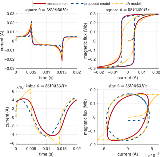
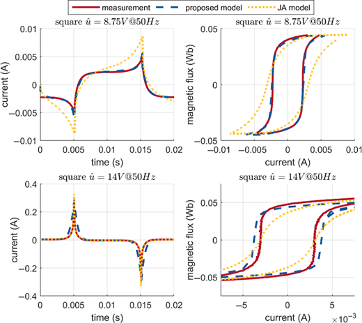
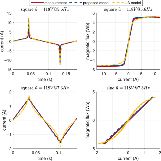
The qualitative visual comparison of the resulting current response and the corresponding hysteresis for the three representative CTs can be seen in Figure 4, Figure 5 and Figure 6.

Both models are able to reproduce the measurements, while the control-oriented model is better at generalizing over a wider range of input settings. This is especially visible for CT$C0$ in Figure 4, where the sinusoidal input $u2$ evokes characteristic saturation currents in the Jiles-Atherton model, whereas the control-oriented model and the measurement show no saturation. This is caused by the selected saturation function. The Jiles–Atherton model uses a hyperbolic cotangent function with limited adaptability. The proposed saturation function (4) of the control-oriented model is more versatile and better at depicting the correct material characteristic.

The overall shape of the hysteresis curve for CT$C2$ in Figure 5 is accurately captured by both the Jiles–Atherton model and the control-oriented model. However, the Jiles–Atherton model overestimates the current amplitude at voltage setting $u3$⁠, while the control-oriented model slightly overestimates it at voltage setting $u4$⁠.

The hysteresis of transformers from cluster $C3$ are generally thinner compared to other clusters, as seen in Figure 6. This is also reflected in the identified parameters of both models, where smaller values for the parameters describing the width of the hysteresis are found. The control-oriented model is capable of accurately describing the current response in the linear range of the material as well as in saturation.

Additionally, to the qualitative visual evaluation, the model is compared quantitatively by calculating the normalised error between the measured current $imes,o$ and the simulated current response $io$ over one period of the input voltage. This quality measure is defined in Schwartze et al. ( 2025b) as follows:

It is calculated at each operation point $o$ corresponding to a voltage setting $uo∈1…6$⁠. The squared error between the simulation and the measurement is integrated over one period. This error is normalized by the integral over the squared measured current. This ensures that the error metric depends less on the amplitude of the current and thus the values at different operation points are comparable. Table 4 shows the calculated error metric for both models at all operation points $uo$ and CTs. It can be seen that the control-oriented model consistently achieves better values in the error metric – with the exception of $u4$ on CT$C2$⁠. The reason for the increased error value is that the model does not estimate the amplitude peak of the current response correctly. A potential solution could be a better fitting saturation function $sx1$ that can more accurately describe the saturation characteristic of this ferromagnetic core material.

In this simulation study, the computational effort of the control-oriented model and the transformer model based on the Jiles–Atherton equations from Albert et al. (2024) is compared. The simulation is performed on an Intel Core i5-8365U CPU @ 1.60 GHz with 16 GB RAM. Both models are implemented in MATLAB/Simulink R2023a (The MathWorks Inc, 2023a). The significant difference between the value of the leakage inductance $Lk$ and the unsaturated main inductance $Lm$ renders solving the parametrized model a stiff problem. This motivates the usage of a stiff solver such as the ODE15s variable step-size solver (The MathWorks Inc,  2023b). For a fair comparison, the same solver settings are selected. The maximum step-size is chosen to be $10-6$ s, which means that the solver can automatically adjust the step-size, up to the specified limit.

To compare the computational effort of the simulation of different transformers, the relative simulation time:

is defined. It is calculated by dividing the computation time $Tc$ that is needed to execute one run of the simulation, with the duration of the simulation $Ts$⁠, i.e. the time instance that is simulated. The value of $Tr$ explains, how much computation time is needed to predict one second of simulation time. A value of $Tr>1$ means that the simulation takes longer than reality. Conversely, a value of $Tr<1$ indicates a simulation that is usable for real-time applications.

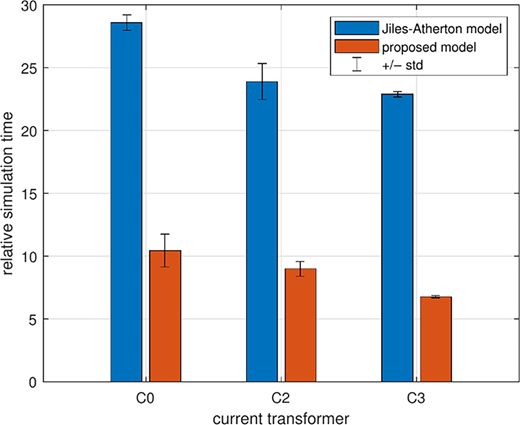
The bar chart in Figure 7 compares the mean relative simulation time $Tr$ for the three selected representative CTs. It can be seen that the relative simulation time for the control-oriented model is significantly shorter compared to the Jiles–Atherton model. Each run-time experiment is performed for 10 consecutive times to minimize random effects introduced by the operating system. By solving the pre-compiled model, the time introduced by the compiler is excluded from the computation time measurement.

The main advantage of the control-oriented model compared to the model based on the Jiles-Atherton equations is the representation of hysteresis. The Jiles–Atherton model is a special implementation of the Duhem hysteresis model (Visintin, 1994), which is given by the differential equation:

where the input to the model is denoted by $u$ and $x$ describes the output. Based on the time-derivative of the input $u˙$⁠, the hysteresis is described by the increasing function $g1u,x$ or the decreasing function $g2u,x$⁠. Therefore, all Duhem-type hysteresis models need the derivative of the input, which is not necessarily available. Thus, for implementation purposes, the derivative is often approximated by a finite difference scheme such that:

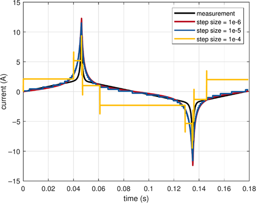
Especially, for noisy inputs or inputs with a large time derivative, such as square waves, this approach can become numerically problematic. In Figure 8, the maximum solver step-size of ODE15s is varied. It is observed that increasing the maximum solver step-size introduces numerical issues which leads to a loss in quality of the predicted output current. To mitigate this numerical issue, the time steps need to be chosen very small, which in turn increases the computational effort and thus the computation time.

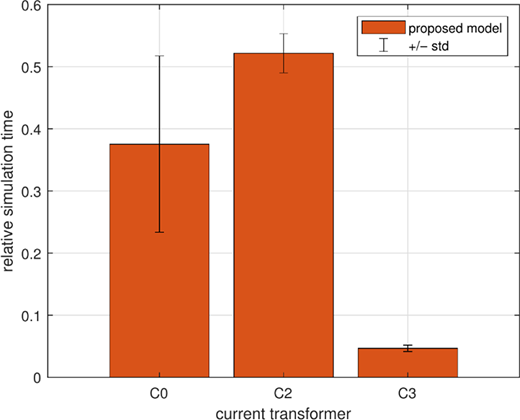
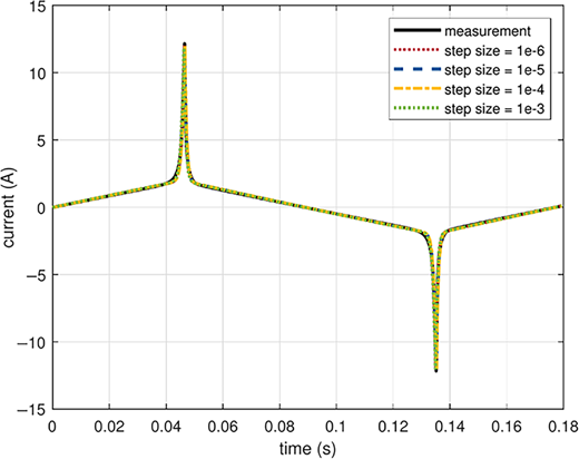
In Figure 9, the same run-time experiment is performed for the control-oriented model. The maximum step-size of the ODE15s is increased to $10-3$⁠, which can be done without any loss of quality in the simulated current response, as demonstrated in Figure 10. The resulting relative simulation time $Tr$ is drastically improved compared to Figure 7. It can be observed that $Tr$ falls below $1$⁠, which means that the computation time is shorter that the simulation time. This allows to apply the control-oriented model in real-time applications where the computed current output $i$ is time critical.

The proposed control-oriented model for inductive transformers can be written in a state-space representation which is especially beneficial for model-based controller design tasks. Additionally, the control-oriented model is valid for arbitrary input signal wave forms. It is validated on a wide range of different transformers, which were chosen based on a comprehensive data analysis. The simulated output current is in good agreement with measurements and other, well-established transformer models. Due to the structure of the proposed control-oriented model the simulation time can be significantly reduced compared to the Jiles–Atherton model, which opens the possibility for real-time applications.

The authors would like to acknowledge the support of the industrial cooperation partner, OMICRON electronics GmbH, for facilitating this study and the experimental analysis.