Diffuse-interface models provide a versatile framework for simulating binary-fluid flows with complex interfacial dynamics, including topological changes and dynamic wetting. Numerical approximation of the underlying Navier–Stokes–Cahn–Hilliard (NSCH) equations is challenging due to spatiotemporal multiscale behavior, -conditional stability and ill-conditioning. The purpose of this work is to evaluate higher-order generalized-α time-integration methods, focusing on the third-order scheme, for approximating the time-evolution of the NSCH equations.
The authors regard the application of higher-order generalized-α methods to the NSCH system. Their two-step single-stage form facilitates temporally varying spatial adaptivity, providing a framework for effectively resolving the spatiotemporal multiscale behavior of the NSCH equations. In addition, generalized-α schemes offer tunable numerical dissipation and built-in error estimates for adaptive time-stepping strategies. A one-dimensional numerical experiment is presented to elucidate the properties of the generalized-α scheme for the NSCH equations and to compare its performance to classical θ-methods.
The generalized-α scheme attains its theoretical asymptotic convergence rate and high accuracy at small time-step sizes, outperforming classical θ-methods. However, at larger time steps, the accuracy of the method deteriorates and nonlinear instabilities arise. Moreover, higher-order generalized-α schemes entail substantial algorithmic complexity for NSCH systems, particularly with non-matching densities and viscosities, due to the systems’ many complex nonlinearities.
Most investigations of time integrators for NSCH systems are limited to first- or second-order schemes. This work is the first to examine higher-order generalized-α methods for the NSCH system exhibiting both their advantages and limitations and providing valuable insights into trade-offs between accuracy, stability, efficiency, versatility and algorithmic complexity of the generalized-α scheme relative to classical time-integration methods.
1. Introduction
Diffuse-interface models offer a powerful modeling framework for intricate binary-fluid flows in science and engineering, in view of their ability to accurately capture complex interfacial dynamics. A key advantage of diffuse-interface models lies in their inherent capability to handle topological changes, such as merging and breakup of interfaces (Khanwale et al., 2022), without the need for ad hoc treatments. In addition, they provide a natural framework for simulating contact line dynamics (Xu et al., (2018; Demont et al., 2026) and can robustly accommodate geometrically complex features (Stoter et al., 2023).
Diffuse-interface models for binary fluids find their origin in the seminal work of van der Waals (1893, 1979), who was the first to describe an interface carrying surface energy as a continuous-transition layer, and of Cahn and Hilliard (1958), who provided the first thermodynamically consistent model for the composition evolution of non-uniform mixtures. The first systematic extension to binary fluids, referred to as model-H, was presented by Hohenberg and Halperin (1977) in the late 1970s. Model-H is an incompressible binary-fluid model, i.e. the mixture velocity is solenoidal. However, it has been specifically derived for binary fluids with uniform mass density, and it is only thermodynamically consistent in this restricted setting. Various extensions of model-H have been presented to account for non-matching component densities, e.g. the quasi-incompressible models by Lowengrub and Truskinovsky (1998) and Shokrpour Roudbari et al. (2018), and the incompressible models by Ding et al. (2007) and Abels et al. (2012). The aforementioned models are collectively referred to as Navier–Stokes–Cahn–Hilliard (NSCH or CHNS) models. An overview and classification of the main characteristics of existing models can be found in Eikelder et al. (2023). In addition, various reformulations (e.g. using different state variables) of these models have been presented, often with the aim of deriving tailored numerical approximation methods that retain certain fundamental properties of the binary-fluid system, such as species conservation and energy dissipation.
Numerical simulation of diffuse-interface models carries several fundamental challenges (Demont et al., 2022; Han and Wang, 2015): (i) spatial multiscale behavior arises due to the extremely thin fluid–fluid interface compared to macroscopic length scales, demanding high resolution; (ii) temporal multiscale behavior stems from the disparity between the fast diffusion dynamics at the interface, slower macroscopic processes and time singularities in topological changes; (iii) -conditional stability imposes severe time-step restrictions tied to a CFL-type condition where the interface displacement per time step is limited to its thickness (), leading to prohibitive computational costs as the sharp-interface limit is approached, i.e. as ; (iv) heterogeneous parameters such as large density and viscosity contrasts can cause instability and ill-conditioning; (v) incompatibility and spurious velocities corresponding to discretization errors that manifest as parasitic flows, with a velocity magnitude that is inversely proportional to the Ohnesorge number and which are, therefore, particularly problematic in low-viscosity regimes; (vi) Ill-conditioning of linear systems complicates the solution of the coupled nonlinear equations due to asymmetry, parameter disparity and subsystem aggregation. Together, these issues present significant barriers to practical and predictive simulations of multiphase systems based on diffuse-interface models, particularly in engineering and scientific applications involving significant parameter variations.
Various methodologies have been proposed to address the aforementioned challenges. Adaptive mesh refinement has proven to be an effective approach to resolving the spatial multiscale behavior of diffuse-interface models (Demont et al., 2022; Garcke et al., 2016; Van Brummelen et al., 2021). To address non-robustness emerging from the temporal multiscale behavior, specific energy-stable time-integration methods have been proposed (Shen and Yang, 2010, 2013; Shokrpour Roudbari et al., 2018; Khanwale et al., 2022; El Haddad and Tierra, 2022; Liu et al., 2023; Garcke et al., 2016). By construction, the energy stability is unconditional in some schemes (Han and Wang, 2015; Garcke et al., 2016; Shokrpour Roudbari et al., 2018; Shen and Yang, 2010, 2013) and conditional in others (El Haddad and Tierra, 2022; Khanwale et al., 2022; Liu et al., 2023). Robustness of the solution process, in the sense of unique solvability of the algebraic system within each time step, is ensured for some of these approaches by monotonicity properties (Han and Wang, 2015) or linearity (Shokrpour Roudbari et al., 2018; Liu et al., 2023; El Haddad and Tierra, 2022; Garcke et al, 2016). In Demont et al. (2022), it was noted that the standard Newton solution procedure fails if the diffuse-interface displacement within one time step exceeds the interface thickness, owing to the fact that the error in the initial estimate provided by the solution in the previous time step then becomes excessively large. This non-robustness can be effectively resolved by means of -continuation, i.e. a continuation procedure in the diffuse-interface thickness, and this -continuation approach is synergetic with adaptive-refinement procedures. The issue of ill-conditioning in NSCH systems can generally be bypassed using a partitioned solution procedure that decomposes the NSCH system into its NS and CH parts (Demont et al., 2022; El Haddad and Tierra, 2022; Garcke et al., 2016; Liu et al., 2023; Shen and Yang, 2013).
By virtue of the preceding advances in computational methodologies, the robustness of time-integration methods for diffuse-interface binary-fluid models has improved significantly. However, the accuracy of energy-stable time-integration schemes is generally limited to first (El Haddad and Tierra, 2022; Shen and Yang, 2010, 2013; Shokrpour Roudbari et al., 2018; Liu et al., 2023) or second (Khanwale et al., 2022; Han and Wang, 2015) order and the artificial numerical dissipation in these schemes in many cases surpasses physical dissipation, unless time steps are applied that are exceedingly small compared to relevant problem-specific time scales, e.g. the period of oscillation of a droplet (Demont et al., 2022). In Demont et al. (2022) the standard second-order Crank-Nicolson scheme, acclaimed for its favorable low numerical dissipation, was applied to the problem of an oscillating droplet, and it was found that without -continuation the robustness of the Newton procedure limits the admissible time step, while with -continuation the accuracy of the Crank–Nicolson scheme is restrictive. This reveals the need for high-order time-integration methods for diffuse-interface binary-fluid models.
In this work, we consider a higher-order generalized- time-integration method for the NSCH equations, with the objective of assessing the properties of such an approach for diffuse-interface binary-fluid flow models. The class of generalized- methods offers higher-order alternatives to conventional two-step schemes such as the -method, which can in principle be extended up to arbitrary order (Behnoudfar et al., 2023, 2021). Generalized- methods hold several advantageous properties that render them promising in the context of the NSCH equations. First, their two-step, single-stage form, as opposed to multi-stage methods such as Runge–Kutta schemes or multi-step methods such as BDFs or Adams–Moulton schemes, facilitates temporally varying spatial adaptivity. Second, in generalized- schemes, the higher-order accuracy is accomplished by means of correction terms based on auxiliary variables corresponding to higher-order derivatives. These correction terms provide an intrinsic a-posteriori error estimate, which can be leveraged in adaptive time-step refinement procedures. Third, the correction stages are linearly implicit and unidirectionally coupled, i.e. each higher-order correction depends on the previous, but not vice-versa. As a result, generalized- schemes generally admit a very efficient implementation. Finally, generalized- methods have tunable numerical dissipation properties.
The remainder of this article is arranged as follows. In Section 2 we introduce the NSCH problem and review relevant numerical solution methods to motivate consideration of the generalized- scheme. Section 3 presents the generalized- method and the resulting weak forms. In Section 4, we present numerical experiments for a prototypical one-dimensional diffuse-interface flow problem pertaining to a uniform translation of the interface, to establish the properties of the third-order generalized- scheme. In addition, we presented corresponding results for two -methods to enable a comparison. Section 5 presents concluding remarks.
2. NSCH model and numerical methods
This section presents the NSCH model as derived by Abels, Garcke and Grün (AGG) (Abels et al., 2012) to describe the dynamics of a mixture of two immiscible incompressible Newtonian fluids separated by a thin-but-finite transition layer. Next, we briefly review the -continuation method used in combination with spatial adaptivity to resolve the spatial multiscale behavior of the NSCH equations and bypass the -dependent time-step restriction in the time-integration process for the NSCH equations.
2.1 Navier–Stokes–Cahn–Hilliard model
In diffuse-interface models, the interface between two immiscible fluids is represented by a finite-thickness transition layer composed of a mixture of both constituents. The fluid species are regarded as being omnipresent and the local composition of the binary fluid is described by an order parameter (or phase-field variable), , where denotes pure species 1 and denotes pure species 2. The AGG NSCH model describes the evolution of the multiphase-flow system in terms of the volume-averaged velocity field, , the pressure, p, the order parameter, and the chemical potential, .
On an open time interval and a spatial domain (), the AGG NSCH equations are given by the following:
The constitutive relations for the relative mass flux , specific to the AGG NSCH formulation, the viscous stress , the capillary stress and the chemical potential are defined as follows:
with the symmetric gradient for vector fields, i.e. . This NSCH system generally admits non-matching densities and viscosities and, accordingly, and . However, to facilitate the presentation in this precursory investigation of the properties of generalized- methods for the NSCH system, we restrict ourselves to matched-density and matched-viscosity scenarios, alluding to the effect of generalizations if appropriate. In the matched-density case, the relative mass flux vanishes and the AGG NSCH equations reduce to the standard model-H (Hohenberg and Halperin, 1977).
The model parameters in equations (1) and (2) involve the interface thickness parameter, and the mobility parameter, . Respectively, these control the diffuse-interface length-scale and the diffusive time scale. The material parameters in equations (1) and (2) are the fluid-fluid surface tension, , mass density, and dynamic viscosity, .
The NSCH system can generally be equipped with various types of boundary conditions, e.g. no-slip conditions (Jacqmin, 2000), (generalized-α) Navier slip conditions (Xu et al., 2018; Demont et al., 2026), dynamic and static contact angle conditions (Jacqmin, 2000; Xu et al., 2018; Demont et al., 2026), etc. For transparency, in the present work, we restrict ourselves to settings in which both the velocity and phase field are subject to stationary Dirichlet conditions on some parts of the boundary, and , respectively, homogeneous traction conditions hold on the complementary part , the phase field satisfies homogeneous Neumann conditions on and satisfies homogeneous Neumann conditions throughout. Denoting by the collected Dirichlet data for and , we define the trial space for the weak formulation of (1) subject to the aforementioned boundary conditions as:
and the test space as its counterpart with homogeneous traces of and on and , respectively. The weak formulation of equation (1) subject to the aforementioned boundary conditions can then be condensed into:
where the bilinear form corresponds to the usual inner-product of its arguments, i.e. for scalar-valued arguments and for vector-valued arguments, and:
Remark 1. For matched densities, the volume term in the trilinear forminequation (5a)is skew symmetric inand. Owing to its skew-symmetric structure, this formulation of the convection operator mitigates spurious energy generation (or dissipation) when the transport fieldis not strictly solenoidal, for instance, when the velocity and pressure are approximated using Taylor–Hood elements; seeLayton (2008).
2.2 Spatial adaptivity with-continuation and high-order time integration
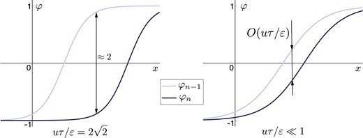
Numerical approximation of equation (4) by a standard Rothe-type approach generally leads to a sequence of nonlinear algebraic equations associated with each time step. Numerical solution of each of these nonlinear algebraic systems by means of a Newton method requires an initial estimate. Conventionally, this initial estimate is obtained from the previous time step. However, this standard procedure leads to -conditional stability: if the diffuse-interface displacement within one time step is large relative to the interface thickness, then the error in the initial estimate is too large, causing breakdown of the Newton procedure; see the illustration in Figure 1. The error in the phase field obtained from a previous time step is in fact approximately for , with u as the transversal velocity of the interface and as the time step. In the limit , the error is ; see Figure 1. Hence, to control the error in the initial estimate in the Newton procedure, the time step must be reduced if the interface thickness is reduced, to ensure that remains sufficiently small.
In Demont et al. (2022), a procedure has been presented to bypass the -dependent time step restriction imposed by the robustness of the Newton procedure. This -continuation method applies a continuation procedure in the interface-thickness parameter, in which the initial estimate for the largest interface thickness parameter, , is obtained from the previous time step, but the initial estimate for each of the subsequent reduced interface thicknesses, ( with ) corresponds to the solution in the current time step at , instead. Accordingly, the time step restriction imposed by the Newton procedure takes the form instead of . The -continuation procedure is synergetic with adaptive spatial refinement based on an a-posteriori error estimate, in that the continuation steps can be combined with the refinement steps in the adaptive process. Such adaptive spatial refinement is instrumental in numerical methods for the NSCH equations, in view of the large gradients that occur in the vicinity of the diffuse interface.
Equipped with the -continuation method, the most stringent time-step restriction derives from the temporal discretization error, related to the temporal-multiscale behavior of the diffuse-interface problem. For instance, for the second-order Crank–Nicolson scheme, the discretization error visibly impacts the results or the robustness of the solution procedure, well before ; see Demont et al. (2022) and also Section 4.2.
Higher-order () time-integration methods can potentially avoid the stringent time-step restrictions of second (or first) order methods. In principle, higher-order methods offer higher convergence rates in the limit . Conversely, for suitably small time steps, this implies that higher-order methods also provide a significant reduction in the discretization error relative to a lower-order scheme. However, when adaptive refinement is used in space to resolve the diffuse interface, the feasibility of various higher-order time-integration schemes can be significantly affected. This is because the diffuse interface must be resolved at every time step and/or stage of the time-integration process, requiring fine spatial resolution over the entire integration sequence. This causes spatial refinement in the length scale to resolve the diffuse interface, in multiple areas near the stages or steps, leading to excessive computational complexity.
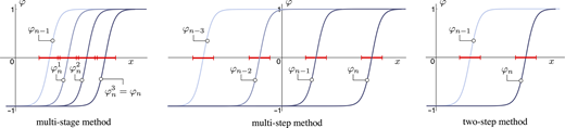
To illustrate the effect of local spatial refinement near the diffuse interface on the computational complexity of higher-order time-integration schemes, Figure 2 illustrates the necessary common refinements for a multi-stage method, a multi-step method and a two-step method such as the generalized- scheme. In multi-stage methods such as Runge–Kutta schemes, the diffuse interface must be resolved in each stage. However, because the approximation space in all stages within one time step must be identical, a common refinement is required that unites the approximation spaces (meshes) for all stages; see the left panel in Figure 2. In addition, a projection step is required at the end of each time step, to avoid the auxiliary refinements for the intermediate stages carrying over to the next time step and, recursively, to all subsequent time steps. For multi-step methods such as BDF, the approximation at time step n involves the computed solutions in time steps , with s the number of steps; see Figure 2 (center). This implies that a common refinement is required that unites the approximation spaces for time step n and all s previous time steps, or the bi-linear and semi-linear forms in (4) must be evaluated for test functions at time level n and trial functions at all time levels (). Both approaches carry a significant computational cost. In addition, auxiliary projection steps may be required to avoid adaptive refinements from carrying over to subsequent time steps. Two-step methods only require a common refinement that unites the approximation spaces for two time levels, namely, n and . Therefore, two-step methods have the potential of being computationally more efficient in comparison to multi-stage and multi-step methods for diffuse-interface models of binary-fluid flows.
3. Third-order generalized- method
Generalized- methods represent a class of higher-order () time-integration methods, alternative to (at most) second-order accurate -methods, designed to provide stable and accurate solutions for time-dependent differential equations. In this work, we focus specifically on the third-order generalized- scheme. This section considers the application of the third-order generalized- scheme to the NSCH equations and elaborates on the different steps in the solution procedure.
3.1 Setup
To provide a setting for a Rothe-type discretization of equation (4), with a generalized- discretization in the temporal dependence, we consider a partition of the time interval . For convenience, we assume the partition to be uniform and denote by the time step. To discretize (4) in the spatial dependence, in turn, we regard a conforming approximation space for time step , subordinate to a mesh-resolution parameter .
In generalized- methods, the state variables of the problem under consideration, , are treated as the primary field, while auxiliary variables are introduced associated with higher-order time derivatives of U. These auxiliary variables are defined by update equations based on Taylor-series expansion and state equations obtained by differentiation of the original weak formulation of the problem under consideration with respect to the temporal dependence. The conforming approximation of the primary variables for the NSCH equations in time step then corresponds to . For the third-order generalized- scheme, the auxiliary variables correspond to the first, second and third-order time derivatives of U. Their conforming FEM approximation at time-step is denoted by , and .
3.2 Application to the NSCH system
In each time step, , the primary variable and auxiliary variables , and in the generalized- scheme are obtained in four sequential steps, which will be elaborated on below.
Step 1
In the first step, the time derivative is extracted from the weak formulation of the NSCH problem (4) with and replaced by suitable approximations:
where we have introduced the condensed notation and . The occurrences of in (6) are implicitly defined in terms of and and via the first update equation:
Hence, is the only unknown in (6). The parameters and in (6) and (7), respectively, are certain user-defined parameters; see Remark 6.
Remark 2. The Dirichlet data foris homogeneous under the standing assumption that the Dirichlet datafor U is stationary. If the Dirichlet data is time-dependent, then the trial space foris subject to non-homogeneous Dirichlet data, which are determined by the prescribed Dirichlet data for via the update equation (7).
Remark 3. The update equation (7) requires datafrom the previous time step. This implies that for, consistent initial data must be constructed for these items. Noting that the NSCH system (1) contains first-order time derivatives forand, the specification of the initial-boundary-value problem requires initial dataand. Given, the initial chemical potential,, can be determined from (1d). In turn,can be derived fromequation (1c). Initial data for pressure and acceleration,and, can be extracted from (1a) subject toequation (1b)differentiated with respect to time, i.e. ∇· = 0. Consistent initial data for higher-order time derivatives can be obtained similarly, based on conditions obtained by differentiating the NSCH equations with respect to time.
Step 2
In the second step, is extracted from the update equation (7), based on data from the previous time step, with index and from step 1. If is a refinement of the approximation space in the previous time step, then the addition in (7) can be executed directly. Otherwise, the identity in equation (7) must be interpreted as a projection. Specifically, in the case of an -projection, follows from:
One may note that the approximation space is not constrained by the Dirichlet data for . The essential boundary conditions on are implicitly accounted for in the construction of ; see Remark 2.
Step 3
The third step produces , based on the weak form equation (4), differentiated in time twice. The differentiation in time leads to a new weak formulation for , which is however significantly more convoluted due to the nonlinearity of equation (4):
where and are abbreviations according to:
The occurrences of in (9) are implicitly defined in terms of , and via the second update equation:
so that is the only unknown in (9). The parameters , and are user-defined; see Remark 6. Similarly to step 1, if the boundary data is time dependent, then the Dirichlet data for is constructed via the update equation (11) and the second-order time derivative of the data, ; cf. Remark 2.
Remark 4. For non-matching mass density and viscosity of the fluid components, the weak formulation (9) forbecomes significantly more complicated, on account of the associated additional nonlinearities. Firstly, the additional termrelated to the relative mass fluxaccording to (2a) must be incorporated in the weak formulation (4), which in turn results in various additional terms inequation (9). Second, the mass density assumes a dependence on the phase field. To account for the fact that the range of the phase field is not generally restricted to, the dependenceis commonly defined by a so-called soft-clipped linear interpolation (Bonart et al., 2019):
with. The mass density appears in the weak formulation as a productwith, which in turn generates a significant number of additional terms inequation (9), requiring higher-order derivatives of the piece-wise expression (12). Third, for non-matching species viscosities, the mixture viscosityis commonly modeled by the Arrhenius mixture-viscosity relation (Arrhenius, 1887;Van Brummelen et al., 2021;Demont et al, 2022):
wherewithandas the molar masses. The nonlinear dependence betweenand the viscous stress tensor,, generates several additional terms in (9). The multitudinous additional terms that occur in (9) as a result of the higher-order derivatives of the additional nonlinear relations associated with the extension to non-matching densities and viscosities, render this extension exceedingly complicated or even unfeasible. It is to be remarked that this complexity is further compounded for higher-order generalized-schemes.
Remark 5. In this manuscript we restrict ourselves to scenarios in which the velocityis sufficiently small to obviate convection stabilization, and we apply the weak formulations in equation (6)and, correspondingly,equation (9)directly. It is to be noted, however, that for larger, the weak formulation (6) must be endowed with additional stabilization terms, which in turn lead to a proliferation of terms inequation (9).
Step 4
The fourth step is analogous to the second step, comprising the construction of via the second update equation (11). This can be accomplished by the -projection:
Analogously to step 2, the approximation spaces do not explicitly incorporate Dirichlet boundary conditions, and these conditions are implicitly accounted for via the construction of boundary conditions on in equation (9) in step three via the second update equation.
Remark 6. The parametersandin the third-order generalized-method are implicitly defined via two user-defined parameters, namely,and, which determine the numerical dissipation and thereby the high-frequency damping (Behnoudfar et al., 2020). Theparameters:
determine the implicit versus explicit character of the scheme. Theparameters in turn determine the twoparameters, which are used in the update equations in solution steps two and four, and which ensure the third-order accuracy of the scheme:
This choice of parameters guarantees an optimal convergence rate and unconditional stability for linear systems (Behnoudfar et al., 2020). For linear problems, the parametersandgovern the spectral radius of the amplification matrix in the high-frequency limit, controlling the numerical dissipation. For nonlinear systems such as the NSCH equations, they act as tunable filters for the high-frequency components of the approximate solution that typically arise from temporal and spatial discretization errors. Smaller values ofintroduce stronger damping, which helps stabilize stiff or convection-dominated flows, while values closer to one preserve more of the transient behavior with minimal artificial dissipation. Hence, the choice ofprovides a flexible means to balance stability, accuracy and temporal smoothness in unsteady flow computations. Jansen et al. (2000) and Liu et al. (2021)proclaim that a spectral radius ofin high-frequency regions generally provides a suitable balance for incompressible Navier–Stokes simulations. In our method, this is obtained by setting. However, for accuracy-sensitive cases,can preserve transient details, at the expense of reduced high-frequency damping. It is to be noted, however, that for sufficiently small time steps, the algorithm’s spectral radius does not bifurcate and the order of accuracy is independent of the selected parameters. To illustrate this aspect,Table A3in Appendix A reports discretization errors for various settings of the stabilization parameters, for the test case presented in Section 4. These results convey that for the considered spatial and temporal resolution, the discretization error is insensitive toand.
Remark 7. The correction terms in the generalized-scheme can be leveraged to obtain an a-posteriori error estimate. Specifically, the expression in the right member of the update equation (8) can be conceived of as a Taylor series expansion ofaround. The Taylor series expansion has remainder ofasforHowever, for admissible values of, it holds that; see Remark 6. Denoting bythe norm associated with the approximation space, the expression:
therefore provides an estimate of the local truncation error. More precisely, under the assumption that the data atis exact, i.e. and U is sufficiently smooth on the interval, it holds that:
while. The error indicatoraccording to (17) is therefore asymptotically exact, i.e. the effectivity indexin the limit. It is to be noted that this asymptotic exactness only holds for the local truncation error, as accumulated errors in the data atwill propagate into the error estimate. We refer to Appendix B for further elaboration and for an analysis of the performance of the error indicator (17) for the numerical experiment in Section 4.
4. Numerical experiment
In this section, we assess the properties of the third-order generalized- scheme for a prototypical model problem, and we compare its performance to two -methods, namely, the implicit-Euler and Crank–Nicolson methods. The model problem pertains to a one-dimensional periodic setting of the NSCH system, with a solution corresponding to a translating (double, to enforce periodicity) interface. For this model, we can construct an analytical reference solution to verify the accuracy of the various time-integration methods. In addition, as the reference solution is characterized by a constant velocity, it is well-suited to assess the impact of the translation velocity of the diffuse interface on the robustness and accuracy of the time-integration schemes.
4.1 Simulation set-up
The considered numerical experiment concerns the convective transport of an equilibrium solution of the NSCH system on a one-dimensional periodic domain . Such equilibrium solutions are hyperbolic tangent functions. On a periodic domain, we require a pair of hyperbolic tangent profiles to enforce periodicity in the translating solution. We define initial conditions for and in accordance with the reference solution:
and (uniformly constant), where is the remainder time, used to enforce periodicity of the reference solution:
The repeating pairs of hyperbolic tangent functions in equation (19) mimic the influence of neighboring profiles of virtually adjacent interfaces. They mitigate continuity issues that would arise due to the mismatch between the hyperbolic tangent profile within the finite domain size and its asymptotic values of and 1.
In addition to the canonical initial conditions for and , the third order generalized- scheme requires initial data for p and , to complete and for and . The initial data for the time derivatives of are obtained via direct time differentiation of the reference solution of the phase field in equation (19). The reference solution of the velocity field is uniform in . Accordingly, the initial conditions for the time derivatives of are homogeneous. Moreover, for uniform in , it follows from equation (1a) that p is uniform in (set to zero) and, hence, the initial conditions for p and its time derivatives are homogeneous. Finally, because corresponds to an equilibrium solution, vanishes uniformly in . Accordingly, homogeneous initial conditions are prescribed for and its time derivatives. It is to be noted that the derivation of the consistent auxiliary initial data that are required by the third-order generalized- scheme is straightforward for the considered reference test case, but not generally; see Remark 3.
The physical parameters and time-stepping parameters used in the numerical experiment are shown in Table 1. They resemble the properties of water at room temperature with a length-scale corresponding to a picoliter droplet. Regarding spatial discretization, we use -continuous cubic splines for the velocity field, phase field and chemical potential, and -continuous quadratic splines for the pressure field. To ensure that the spatial discretization error is at least two orders of magnitude smaller than the temporal discretization error, we use a highly refined mesh consisting of 12,000–48,000 elements. The numerical implementation is performed in Nutils (Van Zwieten et al., 2022).
4.2 Results
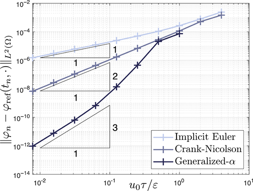
To assess the convergence behavior of the third-order generalized- method in comparison to the Crank-Nicolson and implicit-Euler methods, Figure 3 displays the -norm of the discretization error of the three schemes, , at , versus the normalized time-step size, . One can observe that for sufficiently small time steps, the convergence rate of all three methods is in accordance with theory, i.e. , and for the implicit-Euler, Crank-Nicolson and generalized- method, respectively. For both -methods, the asymptotic convergence behavior occurs for time steps , which corresponds to the time scale at which the diffuse interface moves by approximately its thickness per time step. For the generalized- scheme, however, the asymptotic optimal convergence rate only manifests for time-step sizes . At larger time steps, the error increases rapidly as increases, until it roughly matches that of the Crank-Nicolson and implicit-Euler schemes at . Furthermore, the Crank–Nicolson and implicit-Euler methods appear more robust than the generalized- method for large : for , Newton’s method fails to converge for the generalized- scheme, while it converges effectively for the Crank–Nicolson and implicit-Euler schemes. This nonrobustness of the (linearly) unconditionally stable generalized- scheme is further elaborated in Remark 8 below.
Remark 8. High-order generalized-methods are unconditionally stable for linear problems. This guarantee does however not carry over to nonlinear settings. In practice, we observe that for nonlinear problems and large time steps, Newton’s method (with safeguards) fails to converge. We conjecture that this is primarily due to the breakdown of the high-order Taylor expansions used in the formulation. The auxiliary variables in the generalized-method, corresponding to higher-order time derivatives of the state variables, depend nonlinearly on the state variables and can grow rapidly or lead to severe ill-conditioning of the linear tangent problems in Newton’s method. For instance, the time derivatives of the reference solution in (19) scale asas. Consequently, the Taylor series can diverge, and the residuals in the Newton solver can grow or oscillate, preventing convergence.
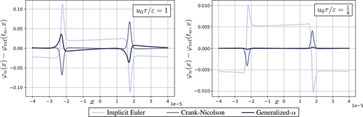
To elucidate the discretization error of the generalized- scheme in comparison to that of the -methods, Figure 4 plots the error in the approximation of the phase field at for time-step sizes and . The time-step size in Figure 4 (left) corresponds to the largest step size for which the Newton procedure converges for the generalized- method, and where the three methods yield similar accuracy; cf. Figure 3. It is notable that the implicit-Euler method shows a significant error throughout the entire domain, while for the Crank–Nicolson method, the error remains confined to a narrow region around the phase transition. For the generalized- method, the error is largest in the vicinity of the diffuse interface, but the error also extends into the single-phase regions. At the smaller time-step size in Figure 4 (right), the benefit of higher-order convergence in the generalized- scheme becomes apparent: its error is substantially lower than that of both -methods.
The computational cost of the generalized- scheme generally exceeds that of the two -methods on account of the auxiliary problems that must be solved. However, as these auxiliary problems are linear, the associated cost is limited. To provide insight into the differences in computational cost of the three schemes, we monitor the wall-clock time and the number of Newton iterations spent per time step. For the generalized- scheme, we moreover record the time spent in solving the auxiliary linear systems. We acknowledge that wall-clock time is only an indirect indicator of computational cost, sensitive to numerous hidden factors. However, the code base for the considered schemes as well as the underlying numerical methods such as integration procedures and linear solvers, are essentially identical. Wall-clock time can therefore serve as a relative indicator for computational cost, enabling a comparison between the different schemes. The results for a single time-step of size are listed in Table 2. We note that the variability of this wall-clock time over the time steps is negligible. Solving the nonlinear NSCH system using a Newton method takes essentially an equal amount of time for the generalized- method and both -methods. The implicit Euler scheme is less expensive per Newton iteration, by virtue of its simple structure, but in this case requires one more Newton iteration per time step than the Crank-Nicolson and generalized- schemes. For the -methods, the nonlinear NSCH system is the only system solved at each time step. Consequently, the total runtime of these schemes corresponds directly to the cost of solving the NSCH system itself. In contrast, the generalized- method requires three additional linear solves. The two update equations associated with equations (8) and (14), incur only minor computational cost by virtue of their simple structure. The time-differentiated auxiliary problem (9), however, requires substantially more time, reflecting its significantly more complex form. Overall, the computational cost of the generalized- method is approximately twice that of the -methods.
Based on the results of this experiment, we conclude that by virtue of its higher-order asymptotic convergence rate, the generalized- method outperforms the Crank–Nicolson method for sufficiently small time-step sizes, in particular, for the considered test case, for . However, due to a steep deterioration of the accuracy of the generalized- scheme in the pre-asymptotic regime, the scheme fails to achieve comparable performance to the Crank–Nicolson method in terms of balancing accuracy and computational expense for . For such larger time-step sizes, both methods yield comparable errors, but the generalized- scheme is more computationally demanding on account of its auxiliary variables. This suggests that the generalized- scheme is only appropriate for applications that require high accuracy. For such applications, its tunable numerical dissipation and built-in error estimation further enhance its potential.
5. Conclusion
The computational approximation of diffuse-interface binary-fluid models presents several fundamental challenges. In this work, we focus on the challenge of efficient and accurate time integration in an effort to combat its inherent temporal multiscale behavior. In earlier work, we introduced the concept of -continuation as a remedy for potential non-robustness of iterative solvers. When this approach is adopted, lower-order time-integration methods transition from being robustness-bound to accuracy-bound in terms of the admissible time-step size. Accordingly, in this work we investigated the feasibility of higher-order time-stepping methods to achieve accuracy when using moderate time-step sizes.
We explored the use of the higher-order generalized- method. In the context of diffuse-interface models, generalized- methods are promising candidates as they are two-step methods, only requiring data from the previous time step to compute the solution in the new time step. This is a crucial property, since diffuse-interface models are commonly combined with spatial adaptivity. A two-step time-integration method requires storage and cross-communication of only two adaptively refined meshes – unlike multi-step or multi-stage methods, where each additional step or stage introduces another refined mesh. Additional properties that render higher-order generalized- schemes a compelling option are their tunable parameters, which provide control over high-frequency numerical dissipation, and the inherent temporal-error estimator, which arises from manipulating the higher-order time derivatives solved for in the scheme.
From an implementation perspective, however, application of higher-order generalized- methods to the NSCH equations proves challenging. Since generalized- methods involve auxiliary (linear) problems based on repeated time differentiation of the governing PDEs with respect to the temporal dependence, the potentially large number of nonlinearities in NSCH models – exacerbated when material properties depend on the order parameter or additional stabilization terms are required – leads to a proliferation of terms. Moreover, the auxiliary state variables resulting from the time differentiation require consistent initial conditions, the derivation of which is unwieldy for nontrivial initial data, in particular for higher-order generalized- schemes. Similarly, for transient data for Dirichlet boundary conditions, the derivation of consistent data for the auxiliary variables is tedious.
To assess the performance of the generalized- scheme for the NSCH equations, we compared the third-order generalized- method with the implicit-Euler and Crank–Nicolson methods for a prototypical one-dimensional NSCH problem corresponding to uniform translation of the diffuse interface. A convergence study confirms their expected asymptotic convergence rates as the time step vanishes. The implicit-Euler and Crank-Nicolson methods (first- and second-order, respectively) each require one solve of a nonlinear system of equations. The third-order generalized- method additionally requires the solution of a linear system of equations, thus resulting in a higher computational cost. As expected, the Crank–Nicolson and generalized- methods consistently outperform the implicit-Euler scheme for sufficiently small time steps. By virtue of its higher-order asymptotic convergence rate, the generalized- scheme delivers superior accuracy compared to both -methods for sufficiently small time-step sizes. However, this superior accuracy of the generalized- scheme does not carry over to larger time steps, due to a steep deterioration of its accuracy in the pre-asymptotic regime. The approximation errors of the three schemes are comparable for time-step sizes for which the diffuse interface moves by approximately its thickness within one time step. Moreover, the generalized- method is less robust, in the sense that Newton’s method fails to converge at larger time-step sizes.
For applications that require very high accuracy, the superior accuracy of the generalized- method, deriving from its higher-order asymptotic convergence rate, outweighs its methodological and computational complexity, compared to the -methods. However, the generalized- method seems non-competitive if moderate accuracy is required and, accordingly, larger time-step sizes are applied. Its additional features – user-controlled dissipation and the inherent error estimation for adaptive timestepping – are potential advantages, the performance and impact of which warrant further investigation.
Acknowledgements
T.B. van Sluijs gratefully acknowledges the financial support through the Industrial Partnership Program Fundamental Fluid Dynamics Challenges in Inkjet Printing (FIP), a joint research program of Canon Production Printing, Eindhoven University of Technology, University of Twente, and the Netherlands Organization for Scientific Research (NWO).
Funding
The Netherlands Organization for Scientific Research (NWO).
References
Appendix 1. Numerical dissipation results
As indicated in Remark 6, the user-controlled parameters determine the numerical dissipation of the generalized- scheme. To elucidate the effect of on the accuracy of the numerical results, Table A1 displays the phase-field error for varying . The results convey that for parameters in the range [0.2, 0.8], the sensitivity of the error is minor. Near the boundaries of the admissibility interval.
[0, 1], the error is more sensitive. For the largest time-step size, the generalized- scheme is unstable for , corresponding to low numerical dissipation.
Appendix 2. time-step error indicator
Remark 7 establishes that the error estimate according to equation (17) provides an asymptotically exact representation of the local truncation error, i.e. the error incurred in one time step under the assumption that the data in the previous time step is exact. In this section we investigate the properties of as an indicator for the incremental error, . Note that the incremental error and the local truncation error are identical if the data in time step is exact, but not otherwise.
We proceed under the assumption that is sufficiently smooth on . To facilitate the exposition, we introduce the Taylor polynomial of degree 4 of at around , in the form:
with . Similarly, we introduce an approximate Taylor polynomial based on the approximate solution:
The triangle inequality yields:
The first term on the right-hand side can be recognized as the error estimate . Under the above mentioned smoothness assumption, the third term can be estimated as as . For the second term, it follows from (B.1) and (B.2) that:
as . The quantity therefore represents an upper bound to the deviation between the incremental error and the error estimate , up to higher order terms. Because the initial data for the generalized- scheme is consistent with the initial data for the NSCH equations, will initially be small, so that the effectivity index of the error indicator is close to 1. As time progresses, however, the error in the approximation of and its derivatives accumulates, leading to an increase of and a deterioration of the effectivity index.
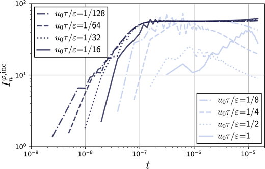
To examine the effectivity of the error indicator in equation (17) as a representation of the incremental error, Figure A1 displays the effectivity index. Specifically, we focus on the incremental error in the phase field, and consider a corresponding effectivity index:
Figure A1 plots versus for different time-step sizes. The results show that the effectivity index is initially close to 1, and that the effectivity index for the first time step approaches 1 as . This is in accordance with the fact that in the first time step, the incremental error is equal to the local truncation error, for which the indicator is asymptotically exact; see Remark 7. The results in Figure A1 moreover indicate that the effectivity index converges in the limit , in the sense that as and such that is fixed, . This limit effectivity index deteriorates as t increases until it reaches a plateau at approximately . The plateau value of approximately 60 indicates that the error estimate yields a loose bound for the actual incremental error. However, the proportionality of the error indicator to the actual incremental error in the limit , suggests that the indicator can still serve to guide an adaptive refinement process.