


This study aims to explore empirical evidence of the impact of greenhouse gas (GHG) emissions on stock market volatility.
Using panel data of 35 Organization for Economic Co-operation and Development countries from 1992 to 2018, we conduct both fixed effects panel model and Prais-Winsten model with panel-corrected standard errors.
The authors document that there is a significant positive relationship between GHG emissions and stock market volatility. The results remain robust after controlling for potential endogeneity problems.
This study contributes to the literature in that it provides additional empirical evidence for the financial risk posed by climate change.
1. Introduction
Over a significant period of time, climate change caused by an increased level of carbon dioxide and greenhouse gases (GHGs) from anthropogenic behaviors has emerged as an important national and social challenge [1]. In this regard, a vast of studies have documented the negative impact of climate change on ecosystems, such as reduced water availability, reduced agricultural yields and increased extreme weather events that ultimately affect human health and well-being (Montgomery, 2017). In addition, climate change poses a large aggregate risk to firms and financial markets (Litterman et al., 2020). Firms have been undergoing a radical shift through increased cost for controlling GHG emissions because of stricter regulations, increased demand for lower-carbon products and increased investor preferences for eco-friendly or sustainable items. Furthermore, more volatile and extreme weather events because of climate change can lead to large financial service providers, such as home mortgage, pensions and life insurance, being unable to shift from their current portfolios, potentially causing financial risks that disturb the stability of the financial market [2].
The risks of climate change that impact financial market can be divided into two categories: physical risk and transition risks. The physical risks are environment events like droughts, floods, storm or rising sea levels. These natural disasters can be a major channel for volatility in the stock market, as they cause uncertainty in the business environment. For example, in an extreme weather event caused by a severe flood, an increase in the number of inundated vehicles can cause insurance companies to incur enormous costs. Prior studies consistently indicate that extreme cold and heat waves have a serious impact on economic activity (Lundgren et al., 2013; Zander et al., 2015; Budhathoki and Zander, 2019). Transition risk arise from changes in policy such as carbon pricing and new technologies such as the growth of renewable energy. For example, there is persistent controversy regarding the appropriate price for carbon emissions. Moreover, uncertainty regarding the extent to which carbon emissions can be limited to decelerate global warning magnifies the uncertainty of climate policies (Barnett et al., 2020). As a result, financial regulators have expressed concerns that investors may be unable to precisely predict the impact of climate change, thereby posing a threat to the overall financial stability (Cœuré, 2018; Carney, 2019). In particular, the risks arising from the uncertainty surrounding climate change regulation and compliance with new regulations can affect business performance (Lee et al., 2015; Nguyen, 2018), consequently reducing the accuracy of analyst forecasts (Pankratz, 2019). The various uncertainties mentioned so far may eventually act in conjunction and increase the volatility of financial markets.
Although we recognize that climate risk would have an impact on firms and financial market, it is difficult to properly understand the impact related to it. This is not only because accurately measuring climate risk is extremely difficult but also because it takes a considerable amount of time for us to feel the impact. While a vast of studies have focus on the association between climate change and financial markets in terms of stock returns, the effects on stock market volatility remains understudied. We contribute to this literature gap by exploring whether equity market volatility rises as exposure to climate change events increases. Furthermore, whereas prior studies linking the effects of climate change on stock prices are limited to specific countries or industries (Oestreich and Tsiakas, 2015; Tian et al., 2016), we perform a cross-country analysis of the Organization for Economic Co-operation and Development (OECD) countries. Extreme climatic hazards, such as flooding, forest fires after severe drought and violent storms, can create climate refugees and destroy economic resources in specific regions or countries; therefore, studies evaluating the impacts of climate change across countries or regions are of great importance. Furthermore, as each country possesses distinct financial systems and policy interventions for climate change, the current comparative study linking climate change and stock market volatility provides significant insight.
To the best of our knowledge, this is the first paper to incorporate the equity market volatility to climate change risk. Using panel data of 35 OECD countries from 1992 to 2018, we document a significant positive relationship between GHG emissions and stock market volatility in OECD markets. We estimate both a fixed effects panel model and Prais–Winsten model with panel-corrected standard errors. The results are robust even after controlling for other factors affecting equity market volatility and endogeneity. Our finding contributes to the academic and policy discussion of the potential financial consequences of climate change-related risks that could constitute a new form of systematic risk with important implication. In this regard, Karydas and Xepapadeas (2019) argue that climate risk potentially leads to extensive financial losses, affecting the stability of the entire financial system.
The remainder of this paper organized as follows: Section 2 describes the data and research design; Section 3 reports the major empirical findings and the discussion of results; and Section 4 concludes the paper.
2. Literature review
In recent years, the theoretical literature on climate change and stock returns continues to grow. For example, Bansal et al. (2017) develop a long-run risks model that accounts for the relationship between temperature-induced natural disasters, future economic growth, and risk. By adopting a dynamic general equilibrium asset pricing model, Barnett (2019) documents the effects of uncertainty climate policy on oil production and prices. Pástor et al. (2021) present an ESG asset pricing frameworks and explain how investor beliefs and preferences about climate change risks fit into the factor model paradigm that dominates empirical asset pricing research. Giglio et al. (2021) construct a measure of attention paid to the risk of rising sea levels coastal US states in housing market and then identify the pricing of this risk. The authors show that low discount rate should be applied to discount the long-run risks of climate change.
Beside theoretical literature, a vast of studies have empirically examined whether climate risk affects stock returns. For example, Karydas and Xepapadeas (2019) incorporate the stochastically time-varying risk of climate change in a dynamic asset pricing model and show that climate change increases equity risk premium. Using carbon emission data of S&P 500 firms disclosed voluntarily, Matsumura et al. (2014) find that firms with higher emissions have lower firm values and firms that choose not to disclose are relatively more penalized. Confounding this, Hsu et al. (2021) document that firms with higher toxic chemical emissions generate higher returns. In particular, a hedge portfolio created from firms with high versus low emission intensity yield, on average, an annual excess return of 4.42%. Pointing out the weak or indirect links between carbon and chemical emissions and climate risk, Berkman et al. (2021) develop firm-specific measures of climate risk exposures based on 10-K disclosures. With these measures, they find that climate change is negatively associated with lower firm value. Using textual analysis method of latent Dirichlet allocation developed by Blei et al. (2003), Faccini et al. (2021) explore whether climate risks are reflected in US stock price. The authors single out four risk factors related to US climate policy, international summits, natural disasters and global warming and find that only the climate policy factor is priced. Their results suggest that only transition risks, which come from domestic political debate on climate change, are priced. Physical risks and transition risk induced by the other component, on the other hand, which may take longer to manifest, are not priced. Most of these studies concentrate on underlying price effects and risk premiums, However, not much has been done on the effect of climate change risk to stock volatility. We contribute to this literature gap by exploring whether equity market volatility rises as exposure to climate change events increases.
3. Materials and methods
3.1 Sample and data description
This empirical study uses a panel data of 35 OECD countries and the data is drawn from OECD database. Because the United Nations Framework Convention on Climate Change (UNFCCC) [3] was adopted in 1992, the sample period 1992–2018 is considered. We focus on each country’s gross direct GHG emissions, excluding emissions or removals from land use, land-use change and forestry. In particular, this proxy includes the total carbon dioxide (CO2 emissions from energy use and industrial processes), methane (CH4 emissions from solid waste, livestock, mining of hard coal and lignite, rice paddies, agriculture and leaks from natural gas pipelines) and nitrous oxide (N2O emissions) emissions. Considering that the amount of GHG emissions varies depending on the size of national economic activities, we use GHG per unit of gross domestic product (GDP) (GHG emission intensity) by dividing the absolute level GHG emissions with GDP. This is a reliable measurement, as OECD also defines GHG emission intensity as GHG per unit of GDP.
Figure 1 indicates the trend of the total GHG emissions among selected OECD countries divided into six groups – Anglo-Saxon countries, Continental Europe, Eastern Europe, Nordic countries, Southern Europe and others. The graph reveals that the total amount of GHG emissions has remained stable over the entire sample period, regardless of the region. Anglo-Saxon countries, such as the USA and Canada, are the highest emitters of the total GHG emissions during the sample period. As Nordic countries are known to pursue the most ambitious climate policies, they have the lowest total GHG emissions among the OECD countries.
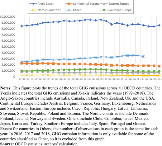
Figure 2 depicts the trend of GHG emissions for the top seven GHG emitters among the OECD countries. The USA has the highest GHG emissions, unrivalled by other countries; this country is followed by Japan. Germany and the UK show a gradual reduction in GHG emissions, whereas Korea and Mexico have increasing emissions. Although China is not included in the sample for this study, at 9,570.8 Mt, it is the largest emitter of CO2 in the world. This is nearly twice the CO2 emissions by the USA, at 4,766.4 Mt, according to the International Energy Agency [4].
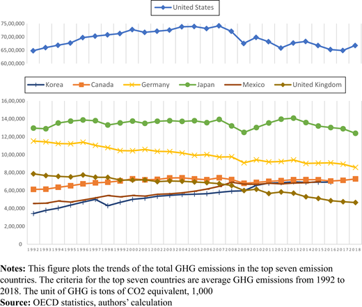
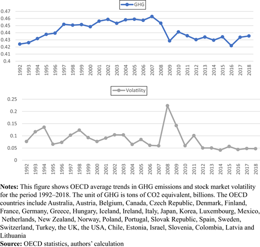
Figure 3 indicates the trend of the average of GHG emission intensity and the average stock market volatility across OECD countries over the sample period. The trend of average GHG emission rises slowly, then suddenly falls during the financial crisis, remaining generally stable thereafter. However, the average volatility of the stock market has been associated with sharp swings in both directions and peaked around the global financial crisis of 2008. Appendix 1 includes the detailed descriptive statistics on GHG emissions from OECD countries used in Figure 3.
Besides GHG emissions, another main variable for our study is equity market volatility, defined as the annualized standard deviation of the natural logarithm of monthly stock indexes for each OECD country (Thomas et al., 2014). We use these indexes because they are powerful indicators for global and country-specific economies, providing a great deal of insight into the country’s economy.
3.2 Research design
We use panel analysis to consider the dynamic relationship between variables and obtain more efficient estimators. Panel analysis also has the advantage of controlling for time-invariant unobserved country characteristics and alleviating the problem of omitted variables. We adopt the following specification:
where t is the time dimension of the data and i is the cross-sectional dimension for individual countries. Independent variable is the total GHG emissions scaled by GDP, because the amount of GHG emissions varies depending on the size of national economic activities (Tucker, 1995). We predict countries with greater GHG emissions have higher stock market volatility and thus, we expect to be positive.
The dependent variable is equity market volatility, measured by the standard deviation of monthly returns using the natural logarithm of monthly share price indices for a particular period. Share price indices are calculated applying the prices of common shares on national stock exchanges, although it is occasionally compiled by agencies such as central banks. The share indices are targeted to be national, all-share or broad price indices and use the closing daily values for monthly data, normally expressed as simple arithmetic averages of the daily data. We consider the share price index 2010 = 100 (reference period) monthly. Considering that all other variables are on an annual basis, we annualize the volatility.
In line with prior literature, we control for a number of country attributes to ensure that the relation between GHG emission and stock market volatility is driven by other factors. We incorporate (lagged volatility) in our panel regression. Given that volatility is highly persistent, most of it can be explained using lagged volatility (Harvey and Whaley, 1992). We use the average market volatility of all OECD countries ( to control the contagion effects from volatility (Baig and Goldfajn, 1999). The rationale behind this is that prior literature shows evidence of common component of cross-country volatility because of deep financial integration and economic cycles (Forbes and Rigobon, 2002; King and Wadhwani, 1990). We expect to be positive. We include the annual inflation rate to capture macroeconomic stability, as inflation is related to volatility of stock price movements because of the risk premium of the interest rate (Bruno, 1993), tax system (Feldstein, 1983) and macroeconomic stability (Engle and Rangel, 2008). To control for depth of the stock market (Bessembinder and Seguin, 1993; Ahn et al., 2001), we add , which is the value of stocks traded in the market. Whereas market depth can affect the positive circle of relationship between transaction costs, liquidity and price volatility through the advantages of economies of scale (Iglesias, 1997; Vittas, 1998), trading with large value or volume could increase market volatility by exaggerating the stock price movements (Nofsinger and Sias, 1999; Sias, 2004). Thus, we do not predict the sign of . We further incorporate (GDP per capita) in our regression, a variable to account for the development of a country (Engle and Rangel, 2008). This variable is typically related to growth rate and terms of trade (Beck et al., 2006) and is a general indicator for capturing differences across countries. We include which represents growth potential (Engle et al., 2013) and is measured by the GDP growth rate in the local currency, to prevent the exchange rate effect. Additionally, volatility can be impacted on the macrolevel by global financial shock or political events and at the country level by country-specific shock or events. Therefore, we add the return of the MSCI world portfolio ( and stock market return of each country ( as control variables. We also include average correlation () of countries’ stock indices (Pollet and Wilson, 2010), measured by averaging the correlation coefficients of countries’ monthly returns by year. Finally, we include and as dummy variables to represent the global financial crisis of 2008 and Paris Agreement of 2015, respectively. These variables have been included because most countries experienced exceptionally high volatility during the global financial crisis, and the Paris Agreement is a legally binding international treaty according to which the international community makes efforts to reduce greenhouse gas emissions. Table 1 presents definitions for the main variables used in the statistical analyses.
Variable definitions
| Variable | Definition | Source |
|---|---|---|
| GHG | Total greenhouse gas emission/GDP | OECD statistics |
| VOL | Volatility, the log of stock market volatility on individual countries i in year | OECD statistics |
| L1_VOL | Lagged volatility, the log of stock market volatility on individual countries i in year | OECD statistics |
| AVOL | Average market volatility of all OECD countries in year t | OECD statistics |
| IF | Annual inflation rate | OECD statistics |
| VST | Natural log of the value of stocks traded in the market | OECD statistics |
| GDP | GDP per head of population. As % of the USA (USA = 100) | OECD statistics |
| GRW | GDP growth rate. GDP is measured in national currency, current prices | OECD statistics |
| MSCI | Yearly return of the MSCI world portfolio | MSCI |
| RET | Yearly returns of individual countries’ stock market index | OECD statistics |
| ACORR | Cross-sectional average correlation across stock indices | OECD statistics |
| D_Crisis | A dummy variable that distinguishes the global financial crisis | |
| D_Paris | A dummy variable that distinguishes after the signing of the Paris Climate Agreement (December 2015) | |
| Forest | Share (%) of forests in the total territorial area | World Bank |
| Fisheries | The aquaculture production in the unit of tons (=1,000 kg) | OECD statistics |
| Feed-in tariffs (FITs) | Prevalent support policies for scaling up renewable electricity capacity | OECD statistics |
Note:s
The sample consists of panel data of 35 OECD countries from 1992 to 2018. All data is obtained from OECD Statistics and World Bank
We conduct a variety of tests to adopt the appropriate panel model specification for our analyses, beginning with a Hausman test to choose between fixed effects or random effect estimator. The results of the Hausman test () allow us to reject the null hypothesis; therefore, the fixed effects model is more plausible for equation (1). Additionally, we test whether there is a cross-sectional dependence among the countries in our model. This is because the panel model assumes that the error terms are independent across cross-sections, and if it exists, the estimated parameters are likely to be inconsistent (Driscoll and Kraay, 1998). Our results reveal that there is a cross-sectional dependence in the model (Pearson’s test of cross-sectional independence = 10.17, = 0.00). Furthermore, we test for heteroscedasticity and serial correlation. In linear panel model, serial correlation biases the standard errors and thus leads the estimator to be less efficient. Accordingly, we conduct Wooldridge test for autocorrelation in panel data and modified Wald test for heteroscedasticity. The results show that there is first-order serial correlation (F-statistics = 59.22, = 0.00) and heteroscedasticity (= 409.10, = 0.00) in the model. If the error terms have autocorrelation and heteroscedasticity in the model, then, as a panel data approach, we can choose either the individual effects model or the panel corrected standard error method (Thomas et al., 2014). Along with the fixed effects model based on the results of the Hausman test, we adopt the Prais–Winsten correlated panels corrected standard errors (Beck and Katz, 1995). We believe this approach can provide more efficient and consistent estimators in the presence of cross-sectional dependence, heteroscedasticity or autocorrelation.
3.3 Descriptive statistics
In Table 2, we present the descriptive statistics for GHG emission intensity, stock market volatility and other control variables used in our analysis. The mean and median of GHG emission intensity is 0.41 and 0.35, respectively, suggesting that GHG intensity tends to be a little right skewed. The average value of volatility is 0.09, much lower than that reported by Thomas et al. (2014), which indicates that a longer time horizon is associated with lower volatility.
Descriptive statistics
| Variables | N | Mean | SD | P1 | p25 | Median | p75 | P99 |
|---|---|---|---|---|---|---|---|---|
| GHG | 1,048 | 0.41 | 0.2 | 0.12 | 0.28 | 0.35 | 0.49 | 1.25 |
| VOL | 978 | 0.09 | 0.09 | 0.02 | 0.04 | 0.07 | 0.11 | 0.32 |
| L1_VOL | 967 | 0.09 | 0.09 | 0.02 | 0.04 | 0.07 | 0.11 | 0.32 |
| AVOL | 1,048 | 0.09 | 0.04 | 0.05 | 0.06 | 0.08 | 0.1 | 0.23 |
| IF | 979 | 5.36 | 21.15 | −0.83 | 1.31 | 2.34 | 3.99 | 66.09 |
| VST | 846 | 24.65 | 2.99 | 17.58 | 22.91 | 24.69 | 27.01 | 31.17 |
| GDP | 1,034 | 67.47 | 28.37 | 19.66 | 47.87 | 70.59 | 82.45 | 175.05 |
| GRW | 1,030 | 0.08 | 0.12 | −0.06 | 0.03 | 0.05 | 0.09 | 0.6 |
| MSCI | 989 | 0.08 | 0.17 | −0.4 | −0.05 | 0.12 | 0.21 | 0.34 |
| RET | 860 | 0.1 | 0.26 | −0.42 | −0.05 | 0.09 | 0.22 | 0.96 |
| ACORR | 989 | 0.43 | 0.16 | 0.12 | 0.32 | 0.43 | 0.55 | 0.73 |
Notes:
The sample consists of panel data of 35 OECD countries from 1992 to 2018. All variables are defined in Table 1
Table 3 presents a Pearson correlation matrix for the variables applied in this study. VOL is positively correlated with GHG at the 1% significance level, consistent with our prediction that GHG emissions are associated with equity market volatility. In addition, VOL is negatively correlated with VST and positively correlated with IF. We also observe a negative correlation between GDP and VOL and a positive correlation between GRW and VOL [5]. Finally, VOL is negatively associated with MSCI and RET, whereas VOL is positively associated with ACORR.
Pairwise correlations
| Variables | (1) | (2) | (3) | (4) | (5) | (6) | (7) | (8) | (9) | (10) | (11) |
|---|---|---|---|---|---|---|---|---|---|---|---|
| (1) GHG | 1.000 | ||||||||||
| (2) VOL | 0.116 (0.000) | 1.000 | |||||||||
| (3) L1_VOL | 0.105 (0.001) | 0.236 (0.000) | 1.000 | ||||||||
| (4) AVOL | 0.126 (0.000) | 0.447 (0.000) | 0.134 (0.000) | 1.000 | |||||||
| (5) IF | 0.063 (0.050) | 0.152 (0.000) | 0.086 (0.008) | 0.052 (0.107) | 1.000 | ||||||
| (6) VST | −0.221 (0.000) | −0.137 (0.000) | −0.155 (0.000) | −0.021 (0.534) | −0.160 (0.000) | 1.000 | |||||
| (7) GDP | −0.317 (0.000) | −0.124 (0.000) | −0.127 (0.000) | −0.055 (0.076) | −0.173 (0.000) | 0.193 (0.000) | 1.000 | ||||
| (8) GRW | 0.215 (0.000) | 0.138 (0.000) | 0.094 (0.004) | 0.011 (0.714) | 0.912 (0.000) | −0.227 (0.000) | −0.322 (0.000) | 1.000 | |||
| (9) MSCI | 0.036 (0.257) | −0.213 (0.000) | 0.168 (0.000) | −0.314 (0.000) | −0.024 (0.459) | −0.034 (0.337) | −0.021 (0.501) | −0.022 (0.490) | 1.000 | ||
| (10) RET | 0.062 (0.067) | −0.094 (0.006) | 0.038 (0.265) | −0.245 (0.000) | 0.313 (0.000) | −0.037 (0.324) | −0.157 (0.000) | 0.481 (0.000) | 0.209 (0.000) | 1.000 | |
| (11) ACORR | −0.211 (0.000) | 0.193 (0.000) | 0.079 (0.014) | 0.296 (0.000) | −0.123 (0.000) | 0.130 (0.000) | 0.017 (0.598) | −0.176 (0.000) | −0.186 (0.000) | −0.248 (0.000) | 1.000 |
4. Empirical results
4.1 Main results
The results of the fixed effects model estimated from equation (1) are presented in Table 4. The joint significance test (F-statistics) indicates that all variables are jointly significant. The coefficient of GHG, central to our analysis, is positively significant at 5% level, indicating that countries with higher GHG emission intensity levels are more likely to have higher volatility in their stock markets. This result is consistent with our argument that the global climate change because of GHG emissions has an impact on the business environment where companies are exposed, consequently increasing the stock market volatility.
Fixed effects panel regression
| Dependent variables: VOL (volatility) | Coefficient | Std. Err | t | P > t |
|---|---|---|---|---|
| GHG | 0.07** | 0.03 | 2.24 | 0.03 |
| L1_VOL | 0.07*** | 0.02 | 4.34 | 0.00 |
| AVOL | 0.72*** | 0.05 | 13.65 | 0.00 |
| IF | 0.00*** | 0.00 | 4.25 | 0.00 |
| VST | 0.01*** | 0.00 | 4.22 | 0.00 |
| GDP | 0.00 | 0.00 | −0.91 | 0.36 |
| GRW | −0.17*** | 0.05 | −3.62 | 0.00 |
| MSCI | −0.02 | 0.01 | −1.43 | 0.15 |
| RET | 0.01 | 0.01 | 1.22 | 0.22 |
| ACORR | 0.02 | 0.01 | 1.23 | 0.22 |
| D_Paris | 0.01 | 0.01 | 1.19 | 0.23 |
| D_Crisis | 0.01 | 0.01 | 0.43 | 0.66 |
| Number of obs. | 718 | |||
| Number of groups | 35 | |||
| R-square within | 0.478 | |||
| R-square between | 0.052 | |||
| R-square overall | 0.239 | |||
| F-statistics | 51.12*** |
Notes:
This table presents the relationship between GHG emissions and stock market volatility, using a panel data of 35 OECD countries. We use the fixed effects panel analysis based on the Hausman test. The dependent variable VOL is the volatility of each OECD country's stock index, and the explanatory variable GHG is the intensity of GHG emissions. All variables are defined in Table 1.
***, **, * denote significant levels at 1, 5 and 10%, respectively
The possible mechanism behind the positive relationship between GHG emissions and stock market volatility is uncertainty in GHG emissions and further uncertainty about the severity and timing of economic and financial losses from climate change. In addition, regulatory climate policies tend to be implemented with high uncertainty (Meah, 2019; Ilhan et al., 2020). The multiple sources of uncertainty make it difficult for investors to precisely quantify the impact of climate change. This could potentially lead to extensive financial losses, exacerbating the stability of the entire financial system (Capasso et al., 2020, Karydas and Xepapadeas, 2019). L1_VOL (lagged volatility) is positively associated with equity market volatility, which is consistent with the autoregressive nature of volatility (Bauwens et al., 2006; Bauer and Vorkink, 2011). AVOL is positively related to the stock market volatility and its coefficient is statistically significant, suggesting that the contagious effects from market volatility exist among OECD countries. This is consistent with the prior research showing that deep financial integration and economic cycle induce a shared component of cross-country volatility (Forbes and Rigobon, 2002; King and Wadhwani, 1990). IF (inflation rates), an indicator of macroeconomic stability (Staff, 1990), has a significantly positive relationship with volatility. This is consistent with prior findings suggesting that inflation can affect volatility by increasing the risk premium of the interest rate (Feldstein (1980; Bruno, 1993). The coefficient of VST, representing the depth of a country's stock market, has a significantly positive value. This is in line with Iglesias (1997) and Vittas (1998) documenting market depth can influence the positive relationship between transaction costs, liquidity and price volatility because of economies of scale. Finally, we find that GRW has a negative coefficient, which is consistent with previous studies showing that stock market volatility tends to be related to the real output growth (Rahman, 2009; Vu, 2015).
The results of the Prais–Winsten regression presented in Table 5 are largely similar to those of the fixed effects regression in Table 4. In particular, the joint significant test (Wald chi2) indicates that all variables are jointly significant and the coefficient of GHG has a positive value at the 1% level, confirming our prediction of a positive relationship between GHG emission intensity and market volatility. Moreover, ACORR (average correlation) becomes positively significant, which is consistent with the literature documenting that an aggregate risk is partially reflected in the average correlation between stock returns (Pollet and Wilson, 2010).
Prais–Winsten regression, correlated panels corrected standard errors (PCSEs)
| Dependent variables: Volatility | Coefficient | Panel-corrected Std. Err | z | P > t |
|---|---|---|---|---|
| GHG | 0.01** | 0.01 | 2.06 | 0.04 |
| L1_VOL | 0.08*** | 0.02 | 5.18 | 0.00 |
| AVOL | 0.70*** | 0.05 | 13.74 | 0.00 |
| IF | 0.00*** | 0.00 | 2.85 | 0.00 |
| VST | 0.00** | 0.00 | −2.08 | 0.04 |
| GDP | 0.00 | 0.00 | −0.31 | 0.75 |
| GRW | −0.07 | 0.05 | −1.40 | 0.16 |
| MSCI | −0.01 | 0.01 | −0.71 | 0.48 |
| RET | 0.01 | 0.01 | 1.10 | 0.27 |
| ACORR | 0.04*** | 0.01 | 3.44 | 0.00 |
| D_Paris | 0.01 | 0.01 | 0.88 | 0.38 |
| D_Crisis | 0.01 | 0.01 | 1.85 | 0.06 |
| Number of obs. | 718 | |||
| Number of groups | 35 | |||
| R-square | 0.521 | |||
| Wald chi2(6) | 627.2*** |
Notes:
This table presents the relationship between GHG emissions and stock market volatility, using a panel data of 35 OECD countries. We use the Prais–Winsten regression, correlated panels corrected standard errors (PCSEs) for controlling cross sectional dependence, autocorrelation and heteroscedasticity based on the Pearson’s test, Wooldridge test and modified Wald test. The dependent variable VOL is the volatility of each OECD country's stock index, and the explanatory variable GHG is the intensity of GHG emissions. All variables are defined in Table 1.
***, **, *denote significant levels at 1, 5 and 10%, respectively
One potential issue related to the test thus far is that both GHG emission and stock market volatility could be endogenously determined. First, reverse causality could be one source of endogeneity. To address this issue, we look into the effects of GHG emission and control variables at year t − 1 on stock market volatility at year t, following Jiang (2008) and Ge and Kim (2014). Results which were not tabulated (coefficient of GHG: 0.12***, t-statistics: 3.21) continue to support the previous findings. Next, endogeneity concerns may rise because of the omitted unobserved country characteristics, such as country policy or business environment, which could result in spurious correlations between GHG emission and stock market volatility. For example, the level of development and commercialization of GHG reduction technologies (Hanova and Dowlatabadi, 2007; Williams et al., 2012) or the timing of activation of the carbon credit system (Gupta, 2011) or carbon taxes (Allan et al., 2014; Luo and Tang, 2014; Goulder, 1992; Tan and Lin, 2020) varies across countries and could simultaneously affect GHG emissions and the entire economy of the country, including the stock market. Furthermore, natural environment (Miles and Kapos, 2008; Van der Werf et al., 2009; Agrawal et al., 2011), fossil fuel-based electric power generation and energy system (Asplund, 2008) or industrial structure (Chang, 2015; Li et al., 2017) can significantly impact both the country’s GHG emission levels and the entire economy.
Additionally, recognizing that GHG emission intensity is the total GHG emissions deflated to GDP, we include GDP and GRW as control variables in our main analysis. Nevertheless, it is still possible that the relationship between GHG and VOL is driven by spurious correlations with GDP. To address this issue, we use a simultaneous equation approach with three equations in column (1) to (3) of Table 6. The parameters of the simultaneous equation model are estimated by a two-stage least square process. The results in column (1) of Table 6 indicate that the potential endogeneity issue does not alter the relation between GHG and VOL. We can notice that GHG still has a significant positive relationship with VOL. In column (2), we include variables that are unlikely to be related to stock market volatility and are likely related with GHG – forest (Miles and Kapos, 2008), fisheries (Cochrane et al., 2009; Parker et al., 2018) and feed-in tariff (FIT) (Fathoni et al., 2014; Sun and Nie, 2015). Forest is defined as the share (%) of forests in the total territorial area, obtained from the World Bank. Fisheries [6] is measured by the aquaculture production, in tons (=1,000 kg), provided by the OECD statistics. FITs [7] are prevalent support policies for scaling up renewable electricity capacity. The OECD data set provides FITs values derived in a manner that are comparable across countries, years and renewable energy subsectors [8]. We use country-level values on the tariff (in US$/kWh) and then derive the sum of the values in subsectors of each country by year. Fisheries and FITs are deflated to GDP in the same way as GHG.
Simultaneous equations
| Dependent variables | VOL | GHG | GDP | |||
|---|---|---|---|---|---|---|
| (1) | (2) | (3) | ||||
| Coefficient | z | Coefficient | z | Coefficient | z | |
| GHG | 1.17*** | 3.49 | −190.85*** | −5.63 | ||
| VOL | −0.22 | −1.49 | ||||
| L1_VOL | 0.21*** | 3.35 | ||||
| AVOL | −1.75 | −1.45 | ||||
| IF | 0.00** | 1.82 | −0.49*** | −4.65 | ||
| VST | 0.02*** | 2.61 | ||||
| GDP | 0.00 | 1.19 | −0.00*** | −3.63 | ||
| GRW | −0.15 | −1.43 | 30.70*** | 3.01 | ||
| MSCI | −0.16** | −2.12 | ||||
| RET | −0.00 | −0.12 | −3.96* | −1.74 | ||
| ACORR | −0.11* | −1.83 | ||||
| Forest | 0.04 | 1.34 | ||||
| Fisheries | −0.04 | −0.17 | ||||
| FITs | −0.07*** | −6.47 | ||||
| Obs. | 373 | 373 | 373 | |||
| R-square | 0.38 | 0.13 | 0.94 | 7 | ||
| Chi-square | 677.02*** | 55.12*** | ||||
Notes:
This table presents the results of simultaneous equations to alleviate endogeneity problem. The main analysis result is in column (1), where the explanatory variable, GHG, still has a significant positive regression coefficient. We include country and year dummy variables in the model. All variables are defined in Table 1;
***, **denote significant levels at 1 and 5%, respectively
The result in column (2) indicates that stock market volatility does not affect GHG emissions, confirming that GHG causes VOL, but VOL does not cause GHG. FITs and Fisheries are insignificantly associated with GHG. The negative relation between GHG emissions and FITs indicates that government subsidies for renewable energy are likely to effectively reduce GHG emissions. In the column (3) of Table 6, where GDP is the dependent variable, we find that countries with lower inflation and higher growth tend to have larger GDP. This negative relationship between GDP and GHG is to be expected, given that the GHG is scaled by GDP.
Finally, we implement a change regression to further confirm our findings, which helps control for the time-invariance factors affecting both GHG emission and equity market volatility. Based on the results from the Hausman test , the random effects linear panel model is adopted. Additionally, we conduct Breusch–Pagan Lagrange multiplier test. The result shows that OLS regression is preferred to random effects panel regression. Accordingly, we regress the change in equity market volatility on the change of the GHG as well as the change of the control variables. As presented in Table 7, the coefficient of GHG is marginally positive, confirming our argument that countries with higher GHG emission likely experience greater stock market volatility.
First-difference estimation model
| Dependent variables: △Volatility | Coefficient | Std. Err | t | P > t |
|---|---|---|---|---|
| △GHG | 0.32** | 0.01 | 2.22 | 0.03 |
| △L1_VOL | −0.11*** | 0.02 | −4.96 | 0.00 |
| △AVOL | 0.00 | (omitted) | . | . |
| △IF | 0.00 | 0.00 | 1.00 | 0.32 |
| △VST | 0.02*** | 0.00 | 3.40 | 0.00 |
| △GDP | 0.00 | 0.00 | 1.64 | 0.10 |
| △GRW | −0.08 | 0.06 | −1.31 | 0.19 |
| △MSCI | 0.00 | (omitted) | . | . |
| △ACORR | 0.00 | (omitted) | . | . |
| △RET | 0.02** | 0.01 | 2.49 | 0.01 |
| D_Paris | 0.09*** | 0.01 | 6.03 | 0.00 |
| D_Crisis | 0.09*** | 0.01 | 6.00 | 0.00 |
| Number of obs. | 681 | |||
| Adj R-squared | 0.51 | |||
| F-statistics | 10.21*** | |||
| Year dummy | Included | |||
| Country dummy | Included |
Notes:
This table presents the result of the first-difference model to address the problem of omitted variables with panel data. We use the OLS regression analysis based on the Hausman test and Breusch–Pagan Lagrange multiplier test. The dependent variable △VOL is the change in the volatility and the explanatory variable △GHG is the change in intensity of GHG emissions. We include year and country dummy variables in the model. All variables are defined in Table 1.
***, **, *denote significant levels at 1, 5 and 10%, respectively
Furthermore, the effect of GHG emissions on stock market volatility is expected to be stronger in countries producing higher GHG emission than in countries with lower GHG emission. This is because the former countries are likely to be more exposed to higher uncertainties related to climate change. Namely, companies in such countries could be more impaired by weather or natural disasters, consequently bringing economic hardships that adversely affect business environment. To check whether the impact of GHG on the stock market varies according to the level of emission intensity, we conduct a subsample analysis. To this end, we classify all countries into higher GHG emitters versus lower GHG emitters by sorting the samples into two groups based on the median of the total GHG emissions by year. Appendix 2 lists the countries with low GHG emission in the left panel and the countries with high GHG emission in the right panel.
Table 8 displays the effect of the changed GHG on the change in stock market volatility for two subsamples. The results show that the coefficient of △GHG is statistically significant only in the sample with higher GHG emissions. This indicates that the positive relationship between △GHG and △VOL is mainly driven by countries with higher GHG emissions, which is consistent with the prospect theory (Barberis and Huang, 2001; Grinblatt and Han, 2005; Kahneman and Tversky, 2013) [9]. Our result is in line with the findings that spillover of volatility arising from unfortunate news is more pronounced, as documented by Koutmos and Booth (1995).
Comparison of countries with high and low GHG emissions
| Dependent variables: △Volatility | Low | High | ||
|---|---|---|---|---|
| Coefficient | t | Coefficient | t | |
| △GHG | 0.11 | 0.47 | 0.53*** | 2.82 |
| △L1_VOL | −0.07*** | −2.68 | −0.22*** | −4.71 |
| △AVOL | 0.00 | (omitted) | 0.00 | (omitted) |
| △IF | 0.00 | 1.15 | 0.00 | 1.11 |
| △VST | 0.01*** | 2.97 | 0.01 | 1.46 |
| △GDP | 0.00 | 0.09 | 0.00 | 1.31 |
| △GRW | 0.11 | 1.04 | −0.21*** | −2.70 |
| △MSCI | −0.16 | (omitted) | −0.09*** | 4.17 |
| △ACORR | 0.00 | (omitted) | 0.00 | (omitted) |
| △RET | −0.00 | −0.06 | 0.04*** | 3.40 |
| D_Paris | 0.01 | 0.46 | 0.07*** | 4.27 |
| D_Crisis | 0.16*** | 6.90 | 0.29*** | 12.76 |
| Number of obs. | 291 | 390 | ||
| Adj R-squared | 0.506 | 0.585 | ||
| F-statistics | 5.29*** | 10.05*** | ||
Notes:
We divide countries into two groups – low/high – based on average GHG emissions by year. This table presents the effect of the changed GHG on the change of stock market volatility. The results indicate that the coefficients of △GHG are statistically significant only in the sample with higher GHG emitters. All variables are defined in Table 7.
***, **, *denote significant levels at 1, 5 and 10%, respectively
5. Conclusion
The aim of this study is to enhance the understanding of the economic consequences of climate change risk on financial markets. Using the panel data of 35 OECD countries from 1992 to 2018, we document the significant positive relationship between GHG emissions and stock market volatility across OECD countries. The results remain significant after controlling for potential endogeneity issues. In particular, by showing that changes in GHG emissions increase changes in stock market volatility, we further confirm our argument that climate change risks can increase equity market volatility. Finally, we observe that the relationship between changes in climate change risk and volatility are mainly driven by high GHG emitters.
Although this study explores whether GHG emissions influence stock market volatility, we acknowledge that this relation, rather than a direct link, could be, in fact, driven by several other mechanisms or factors acting in between them such as uncertainty. Nevertheless, the findings of our paper are shedding light on the broader indirect impact of climate change on financial market in terms of equity market volatility. Along with recent literature by Battiston et al. (2017), Capasso et al. (2020) and Karydas and Xepapadeas (2019), our results indicate that the exposure to climate change risk could potentially result in systematic threads to global financial stability, unless the market precisely estimates the exposures of climate change risk.
To ensure that climate change risks do not pose a threat to financial stability, firms and investors should better manage their climate risk exposures in a way that takes into account not only the direct exposures caused by climate change but also the wider indirect exposures. In particular, institutional investors need to develop better metrics of climate risk exposure, which allow for better pricing and hedging of climate risk. Besides, we suggest that regulators enforce companies mandatory disclosure on financial information about their exposure to climate risks. Climate-related disclosure requirements would enable market pricing that reflects the cost of climate risks inherent in various asset classes, which could reduce the degree of error in estimating equity pricing.
OECD countries' GHG emissions to GDP from 1992 to 2018
| Variable | Obs | Mean | Std. | Min | Max |
|---|---|---|---|---|---|
| Australia | 27 | 0.636 | 0.106 | 0.480 | 0.840 |
| Austria | 27 | 0.260 | 0.037 | 0.200 | 0.310 |
| Belgium | 27 | 0.360 | 0.085 | 0.250 | 0.490 |
| Canada | 27 | 0.582 | 0.094 | 0.450 | 0.730 |
| Chile | 25 | 0.343 | 0.044 | 0.280 | 0.410 |
| Colombia | 23 | 0.313 | 0.036 | 0.250 | 0.380 |
| Czech Republic | 27 | 0.605 | 0.175 | 0.370 | 0.970 |
| Denmark | 27 | 0.311 | 0.086 | 0.180 | 0.470 |
| Estonia | 27 | 0.793 | 0.243 | 0.520 | 1.200 |
| Finland | 27 | 0.393 | 0.100 | 0.250 | 0.570 |
| France | 27 | 0.248 | 0.047 | 0.180 | 0.330 |
| Germany | 27 | 0.334 | 0.065 | 0.230 | 0.450 |
| Greece | 27 | 0.432 | 0.053 | 0.350 | 0.500 |
| Hungary | 27 | 0.368 | 0.100 | 0.240 | 0.540 |
| Iceland | 27 | 0.394 | 0.060 | 0.290 | 0.500 |
| Ireland | 27 | 0.400 | 0.158 | 0.180 | 0.700 |
| Israel | 16 | 0.370 | 0.049 | 0.290 | 0.440 |
| Italy | 27 | 0.259 | 0.029 | 0.210 | 0.300 |
| Japan | 27 | 0.310 | 0.026 | 0.250 | 0.350 |
| Korea | 25 | 0.486 | 0.071 | 0.390 | 0.610 |
| Latvia | 27 | 0.392 | 0.158 | 0.240 | 0.760 |
| Lithuania | 27 | 0.440 | 0.162 | 0.250 | 0.740 |
| Luxembourg | 27 | 0.320 | 0.107 | 0.200 | 0.600 |
| Mexico | 24 | 0.378 | 0.018 | 0.350 | 0.410 |
| Netherlands | 27 | 0.324 | 0.077 | 0.220 | 0.470 |
| New Zealand | 27 | 0.640 | 0.111 | 0.460 | 0.860 |
| Norway | 27 | 0.212 | 0.033 | 0.160 | 0.270 |
| Poland | 27 | 0.688 | 0.255 | 0.390 | 1.200 |
| Portugal | 27 | 0.275 | 0.030 | 0.230 | 0.320 |
| Slovak republic | 27 | 0.500 | 0.204 | 0.260 | 0.950 |
| Slovenia | 27 | 0.401 | 0.090 | 0.270 | 0.550 |
| Spain | 27 | 0.285 | 0.044 | 0.210 | 0.340 |
| Sweden | 27 | 0.197 | 0.057 | 0.130 | 0.290 |
| Switzerland | 27 | 0.146 | 0.017 | 0.130 | 0.180 |
| Turkey | 27 | 0.322 | 0.033 | 0.260 | 0.370 |
| UK | 27 | 0.328 | 0.104 | 0.180 | 0.530 |
| USA | 27 | 0.524 | 0.103 | 0.370 | 0.700 |
Note:
In the panel analysis of this study, two countries (Latvia and Lithuania) are excluded because of the limitation of information on variables other than GHG, and therefore, the number of observations is different from the table above
List of countries with low/high GHG emissions
| Countries with low GHG emissions | Countries with high GHG emissions |
|---|---|
| Austria (25), Chile (21), Denmark (27), Finland (27), Greece (2), Hungary (27), Iceland (27), Ireland (27), Luxembourg (27), New Zealand (27), Norway (27), Portugal (27), Slovak Republic (27), Sweden (27), Switzerland (27), Estonia (27), Israel (27), Slovenia (27) | Australia (27), Austria (2), Belgium (27), Canada (27), Chile (4), Colombia (23), Czech Republic (27), France (27), Germany (27), Greece (25), Italy (27), Japan (27), Korea (25), Mexico (24), Netherlands (27), Poland (27), Spain (27), Turkey (27), UK (27), USA (27), Chile, public |
Notes:
The criterion for the classification of low/high climate change risk groups is GHG emissions, not GHG emissions to GDP. The high group is countries with high GHG emissions based on the median by year, and the low group is the countries with high GHG emissions based on the median by year. The values in parentheses are the number of times the country was included in the low or high group during the sample period
Notes
A recent report issued by the Intergovernmental Panel on Climate Change indicates that human activities have caused an increase in global warming by approximately 0.2°C compared to preindustrial (over the 1850–1900) levels. This report is significantly alarming, cautioning that if this trend continues to grow at the present rate, global warming is likely to increase by 1.5°C between 2020 and 2030.
For example, Pacific Gas, an electricity provider in California, filed for bankruptcy protection in January 2019 because of the large damages caused by wildfires over two years, amounting to billions of dollars in liability costs.
The UNFCCC is an international environmental treaty seeking to reduce atmospheric concentrations of GHG. Its aim is to prevent a dangerous anthropogenic interference with the earth’s climate system.
China is the country with the largest GHG emissions . we exclude it from this study because China does not belong to the OECD and it is difficult to obtain time series of data including GHG emission information. www.iea.org However.
We further examine the variance inflation factor (VIF) and find no significant multicollinearity issue in our analyses. For example, the largest VIF is 5.5 for GDP and the average VIF is 2.6.
Production of fish, crustaceans and molluscs are expressed in live weight, which is the nominal weight of the aquatic organisms at the time of capture. The harvest of aquatic plants is specified in wet weight (OECD statistics).
They are market-based economic instruments, which typically offer long-term contracts that guarantee the price to be paid to a producer of a predetermined source of electricity per kWh fed into the electricity grid.
Subsectors are solar PV, wind, small hydro, biomass, waste, geothermal and marine.
According to the prospect theory, investors react asymmetrically to bad and good information.

