

The purpose of this paper is to examine the impact of structural breaks on the conditional variance of carbon emission allowance prices.
The authors employ the symmetric GARCH model, and two asymmetric models, namely the exponential GARCH and the threshold GARCH.
The authors show that the forecast performance of GARCH models improves after accounting for potential structural changes. Importantly, we observe a significant drop in the volatility persistence of emission prices. In addition, the effects of positive and negative shocks on carbon market volatility increase when breaks are taken into account. Overall, the findings reveal that when structural breaks are ignored in the emission price risk, the volatility persistence is overestimated and the news impact is underestimated.
The authors are the first to examine how the conditional variance of carbon emission allowance prices reacts to structural breaks.
1. Introduction
Structural breaks in volatility (i.e. volatility shifts) are found to characterize the volatility dynamics of many conventional assets such as equities (Stărică and Granger, 2005), commodities (Ewing and Malik, 2017) and currencies. If they are not properly taken into account, they can lead to over-persistent GARCH models (Hillebrand, 2005), affecting volatility forecasts (Stărică and Granger, 2005). While the effect of structural breaks on the modeling and forecasting of the volatility of many assets has been empirically examined, there is very limited evidence of that effect in the carbon emission market.
The carbon emission trading scheme has been remarkably efficient in reducing greenhouse gas (GHG) emissions (Zhang and Sun, 2016; Ji et al., 2018; Zhang, Li, Hao and Tan, 2018; Zhang, Liu and Xu, 2018)[1], leading to broad implications for environmental policy, institutional investors and industries across various sectors[2]. While carbon allowances have emerged as a financial asset, they are characterized by high volatility (Creti and Joëts, 2017), and can be subject to shifts. This has raised concerns among market participants about suitable risk tools to deal with the modeling and forecasting of price volatility. Numerous articles explore the volatility dynamics of carbon allowance prices. Paolella and Taschini (2008) show that the employment of a standard GARCH process in the market for emission allowances provides accurate one-day ahead VaR forecasts. Benz and Truck (2009) use different GARCH models to study the short-term spot price behavior of carbon allowance prices. Their findings suggest that the GARCH methods adopted are suitable for capturing important statistical properties. Chevallier (2011) indicates the presence of outliers in the volatility of carbon prices via GARCH-based models and argues that yearly compliance events, and growing uncertainties in post-Kyoto agreements, may be among the reasons for the instability in the volatility of carbon allowance prices. Rittler (2012) employs multivariate GARCH models in order to estimate the volatility spillover effects amongst the spot and futures allowance markets during the Phase II period. The study reveals that the futures market sends volatility to the spot market. Byun and Cho (2013) focus on the volatility forecasting of carbon futures and find that GARCH-type models have a better performance than implied volatility and the k-nearest neighbor model. Spiesová (2016) examines the conditional variance of carbon emissions prices using various GARCH models. Dhamija et al. (2017) stress the suitability of applying asymmetric GARCH models for modeling the volatility of carbon allowance prices. Dutta (2018) shows that time-varying jumps occur in the emission price series and play an important role in modeling volatility.
The European Union Allowance (EUA) market has become a particularly important sector, representing more than 80 percent of the global carbon emission market (Tian et al., 2016; Dutta, 2018). The participants in the EUA market have increased in number, and previous studies provide evidence for its utility for hedging portfolio risk (Viteva et al., 2014; Zhang and Sun, 2016). Given that financial time series are often characterized by structural changes in volatility (Stărică and Granger, 2005; Hood and Malik, 2018), one can argue whether such structural breaks are also present in EUA prices and, importantly, whether they can affect the volatility modeling and forecasting of EUA prices.
Our work attempts to address this gap in the related literature by modeling and forecasting the volatility (or risk) of the EUA prices after accounting for structural breaks. Specifically, we deal with the presence of structural breaks, and conduct volatility forecast evaluation and value-at-risk (VaR) evaluation.
Methodologically, we detect the presence of structural breaks in the allowance market volatility (Inclan and Tiao, 1994), incorporate the breaks detected into the conditional variance along the line of Ewing and Malik (2017), and then assess whether GARCH models with structural breaks exhibit better forecasting performance than GARCH models without structural breaks (Kanas, 2013). In doing so, we use asymmetric GARCH processes (EGARCH and GJR-GARCH) to model the asymmetric volatility in emission prices and make related inferences about how good and bad news impact the EUA market volatility under structural breaks. We also consider the effects of structural breaks on the VaR measures (Charles and Darné, 2014). Such rich analyses add to previous studies modeling the volatility of carbon emissions with GARCH without accounting for structural breaks (e.g. Paolella and Taschini, 2008; Benz and Truck, 2009; Rittler, 2012; Spiesová, 2016; Dhamija et al., 2017).
The current paper is related to two strands of research in the carbon market. The first considers the prediction and modeling of carbon price volatility by considering spillovers from other markets such as energy markets (Zhang and Sun, 2016; Wen et al., 2017; Ji et al., 2018). The second considers the dynamic behavior of carbon prices (e.g. Zhang, Li, Hao and Tan, 2018; Zhang, Liu and Xu, 2018). In contrast, this study attempts to refine the modeling and forecasting of carbon price volatility by considering the presence of structural breaks emanating from extreme events. Importantly, unlike Zhang, Li, Hao and Tan (2018) and Zhang, Liu and Xu (2018), our focus is on volatility, which represents the second component of price return distribution. As argued by Christoffersen and Diebold (2000), volatility plays a more important role in asset pricing and risk management than the first moment of the price return distribution.
The findings of our empirical analyses indicate that structural changes in the variance of emission prices should be considered when modeling and forecasting the volatility of the EUA market. Otherwise, inferences about the volatility of the EUA market might be misleading. In fact, after accounting for the potential structural breaks, a significant drop is observed in the volatility persistence of emission prices. Furthermore, the effect of positive and negative innovations on EUA market volatility increases under structural breaks. Finally, the forecast performance of GARCH models improves when structural changes in the emission price variance are taken into account.
2. Data
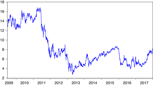
We use daily spot prices of EUA from July 1, 2009 to December 31, 2017, consisting of 2,218 daily observations. Prices are collected from DataStream. Notably, the EU ETS involves three phases: Phase I spans January 2005 to December 2007; Phase II is January 2008 to December 2012; and the EU ETS is currently in Phase III which started in January 2013. Following Tian et al. (2016) and Dutta (2018), our sample period does not cover Phase I because allowance prices at the end of that phase converged to 0 (Tian et al., 2016; Dutta, 2018). Figure 1 shows the emission price index for the sample period under study.
Summary statistics of EUA daily price returns are given in Table I. Price returns exhibit more volatility in Phase III than Phase II. The value of kurtosis is higher than 3 in all cases, suggesting that the distribution of returns is leptokurtic. Except in Phase II, all return series are negatively skewed, suggesting a risk of left tail events. In all cases, the distribution of returns departs from normality, as evidenced by the Jarque–Bera statistics.
Summary statistics
| Mean | SD | Skewness | Kurtosis | Jarque–Bera | |
|---|---|---|---|---|---|
| Full | −0.0093 | 1.3522 | −1.1425 | 26.252 | 50429.29* |
| Phase II | −0.0329 | 1.1000 | 0.2177 | 8.071 | 985.54* |
| Phase III | 0.0071 | 1.5047 | −1.4866 | 27.611 | 33365.54* |
Notes: In this table, we provide summary statistics for daily returns of the emission allowance price index. The statistics are obtained for both full and subsamples. *Statistical significance at 1 percent level
Based on the stationarity tests, specifically the augmented Dickey–Fuller (ADF) and Phillips–Perron (PP) tests, Table II shows that all EUA price series are non-stationary at levels, whereas their return series are stationary.
Results of ADF and PP tests
| ADF tests | PP tests | |||
|---|---|---|---|---|
| Level | First difference | Level | First difference | |
| Full | −1.60 | −34.98* | −1.59 | −46.03* |
| Phase II | −0.62 | −29.10* | −0.64 | −29.08* |
| Phase III | −2.12 | −28.24* | −2.17 | −36.09* |
Notes: In this table, we present the results for the ADF and PP tests applied to both full and subsamples. *Statistical significance at 1 percent level
However, Perron (1989) highlights the need to consider the presence of structural breaks while testing the stationarity of time series. We therefore apply the structural break ADF test and report the results in Table III. They show that EUA prices become stationary at levels when structural breaks are considered. Notably, the results confirm that the three return series are stationary.
Results of unit root testing with structural breaks
| Levels | First difference | |
|---|---|---|
| Full | −5.34* | −46.70* |
| Phase II | −4.36 | −29.76* |
| Phase III | −3.10 | −28.82* |
Notes: In this table, we apply the ADF test accounting for structural break points. The test is applied to both full and subsamples. *Coefficient is statistically significant at the 1 percent level
3. Methods
3.1 GARCH models
The ability of GARCH models to accurately forecast the volatility of financial variables cannot be overstated (e.g. Kang et al., 2009). As indicated in the introduction section, this paper uses both symmetric and asymmetric GARCH processes to model and forecast the risk of EUA prices. Specifically, we employ the symmetric GARCH model (Bollerslev, 1986) and two asymmetric models, the exponential GARCH (EGARCH) model (Nelson, 1991) and the threshold-GARCH (TGARCH) model (Glosten et al., 1993)[3].
The mean equation is given by:
where, rt refers to the daily log return of the carbon emission price at time t. The error term εt is assumed to follow a normal distribution with 0 mean.
The equation of the GARCH (1, 1) model has the form:
where α and β are GARCH parameters, denotes the conditional variance, stands for the volatility news at time t−1. The persistence of volatility is given by α + β.
The TGARCH model of Glosten et al. (1993) is defined as:
where, St−1 indicates a dummy variable taking the value 1 when εt−1 is negative and 0 otherwise.
Asymmetry is said to be present when H0:γ = 0 does not hold. The persistence of volatility amounts to α + β + (1/2)γ.
The EGARCH model assumes the form:
where γ refers to the asymmetric parameter.
3.2 Detecting and dealing with structural breaks
Following Inclan and Tiao (1994), we detect the presence of multiple breaks in the unconditional variance of the EUA market via the iterated cumulative sum of squares (ICSS) algorithm. We augment the GARCH model with structural breaks by adding dummy variables taking a value of one from each point of structural break in variance onwards and 0 elsewhere (Ewing and Malik, 2017). Accordingly, Equation (2) is extended to become Equation (5) and the null hypothesis of no breaks at 5 percent significance level is tested:
As in Ewing and Malik (2017), D1, …, Dn represent the dummy variables that take the value of one for the break periods and 0 elsewhere. The same extension and tests are applied to the two asymmetric GARCH specifications, formulated in Equations (3) and (4).
3.3 Volatility forecast evaluation
We investigate whether including structural breaks in the GARCH models can improve the volatility forecasts for EUA prices. Such an investigation represents an important input for option pricing and risk management decisions. To this end, we follow Kanas (2013) by considering the following regression:
where is the realized volatility[4] of emission prices at the next period, represents the volatility forecast at time t and ξt represents the forecast residual. In fact, is proxied by either the conventional GARCH forecast or extended GARCH forecast; whereas the forecast performance across the various GARCH models is compared based on R2 values.
As a robustness check, we calculate the root mean square error (RMSE) and mean absolute error (MAE) statistics and verify whether considering structural breaks in the GARCH model improves the volatility forecasts for the EUA market. These statistics are defined as follows:
3.4 VaR evaluation
To further study the implications of including structural breaks in the conditional variance of EUA prices, we consider the VaR measure that represents a quantile of the profit–loss distribution (Charles and Darné, 2014). Specifically, we assess whether GARCH models with structural breaks lead to more accurate estimates of the VaR than GARCH models without breaks. We do this for both standard and asymmetric GARCH models. To this end, we first compute the VaR measure as follows:
We then compare the VaR of GARCH models with structural breaks and the VaR of GARCH models without structural breaks via breach frequencies[5]. If the realized breach frequency (failure ratio) of the VaR of the GARCH model with structural breaks does not exceed the selected 5 percent probability level (of that in the VaR), and, importantly, it is lower than the VaR of the GARCH model without structural breaks, we conclude that accounting for structural breaks leads to a more accurate estimate of the VaR measure.
4. Empirical results
4.1 Outlier detection
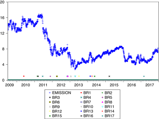
Application of the ICSS algorithm detected 17 structural breaks in the EUA price index. Figure 2 shows the price series with structural breaks, which are generally the consequences of economic and political events such as financial crises, wars, etc (Chevallier, 2011).
4.2 Results of GARCH models
Results from the baseline GARCH model without structural breaks (Equation (2)) and the extended model incorporating structural breaks (Equation (5)) are presented in Table IV. They show that the GARCH parameters are highly significant. The sum of α and β reveals strong evidence of volatility persistence. Therefore, the next period’s volatility is affected by today’s return, which suggests that the future volatility of the EUA prices depends upon the current levels of EUA returns.
Estimates of GARCH (1, 1) model
| Standard GARCH | Extended GARCH | |||
|---|---|---|---|---|
| Parameters/models | Estimates | SE | Estimates | SE |
| ω | 0.0130* | 0.0023 | 0.0946* | 0.0144 |
| α | 0.1153* | 0.0074 | 0.1372* | 0.0149 |
| β | 0.8886* | 0.0063 | 0.7642* | 0.0208 |
| Persistence | 1.0039 | 0.9014 | ||
| Log likelihood | −3,355.48 | −3,280.97 | ||
| AIC | 3.032 | 2.980 | ||
| BIC | 3.045 | 3.034 | ||
Notes: This table shows the estimates of the GARCH (1, 1) process. The extended GARCH model incorporates structural breaks. Persistence is measured as α + β. AIC and BIC refer to Akaike and Bayesian information criteria. *Coefficient is statistically significant at 1 percent level
Further results show that the degree of volatility persistence decreases when structural changes are taken into consideration. For instance, the estimates from the extended GARCH model indicate a significant drop in volatility persistence (i.e. α + β).
The coefficient estimates of the asymmetric GARCH models, exhibited in Tables V and VI, reveal that taking structural breaks into account plays a vital role in modeling EUA price volatility. As with the symmetric case, there is a significant drop in the persistence of volatility for the two asymmetric GARCH processes.
Estimates of TGARCH model
| Standard TGARCH | Extended TGARCH | |||
|---|---|---|---|---|
| Parameters/models | Estimates | SE | Estimates | SE |
| ω | 0.0137* | 0.0024 | 0.0987* | 0.0143 |
| α | 0.0910* | 0.0086 | 0.0956* | 0.0154 |
| β | 0.8855* | 0.0063 | 0.7586* | 0.0207 |
| γ | 0.0546* | 0.0125 | 0.0919* | 0.0235 |
| Persistence | 1.0038 | 0.9001 | ||
| Log likelihood | −3,351.34 | −3,276.38 | ||
| AIC | 3.030 | 2.976 | ||
| BIC | 3.045 | 3.033 | ||
Notes: This table shows the estimates of the TGARCH process. The extended TGARCH model incorporates structural breaks. Persistence is measured as α + β + (1/2)γ. AIC and BIC refer to Akaike and Bayesian information criteria. *Coefficient is statistically significant at 1 percent level
Estimates of EGARCH model
| Standard EGARCH | Extended EGARCH | |||
|---|---|---|---|---|
| Parameters/models | Estimates | SE | Estimates | SE |
| ω | −0.1539* | 0.0084 | −0.1762* | 0.0197 |
| α | 0.2155* | 0.0116 | 0.2465* | 0.0231 |
| β | 0.9868* | 0.0018 | 0.8870* | 0.0126 |
| γ | −0.0335* | 0.0076 | −0.0485* | 0.0143 |
| Persistence | 0.9868 | 0.8870 | ||
| Log likelihood | −3,357.80 | −3,286.07 | ||
| AIC | 3.035 | 2.985 | ||
| BIC | 3.051 | 3.042 | ||
Notes: This table shows the estimates of the EGARCH process. The extended EGARCH model incorporates structural breaks. Persistence is measured as β. AIC and BIC refer to Akaike and Bayesian information criteria. *Coefficient is statistically significant at 1 percent level
Furthermore, the findings of both TGARCH and EGARCH models confirm the existence of asymmetric volatility effects, implying that positive and negative innovations would have heterogeneous impacts on volatility. The coefficient measuring the effects of good and bad news increases significantly when structural breaks are taken into account (see Table VII). These results suggest that for the TGARCH model, for instance, the effect of bad news amounts to 0.145 when breaks are overlooked and 0.186 when breaks are considered. Studying the Chinese carbon market, Zhang, Li, Hao and Tan (2018) and Zhang, Liu and Xu (2018) find evidence of asymmetry, but volatility seems to be more sensitive to good news than bad news.
The magnitude of news impact on volatility
| Standard models | Extended models | |
|---|---|---|
| Panel A: TGARCH process | ||
| Bad news | 0.145 | 0.186 |
| Good news | 0.091 | 0.096 |
| Panel B: EGARCH process | ||
| Bad news | 0.248 | 0.294 |
| Good news | 0.182 | 0.198 |
Notes: In the case of TGARCH models, the effects of good and bad news are α and α + γ respectively. In the case of EGARCH models, the effects of good and bad news are α + γ and α−γ respectively. Extended models incorporate structural breaks
The significance of considering the presence of structural breaks while modeling EUA price returns is further supported by the log likelihood statistic along with other penalized-likelihood criteria such as the AIC and BIC. In fact, when considering structural breaks, the likelihood statistic tends to increase and the AIC and BIC values seem to decrease. Overall, the results indicate that, under structural breaks, standard GARCH models should not be adopted.
4.3 Volatility forecasting performance
Moving to the assessment of whether considering structural breaks in the GARCH models can improve the volatility forecasts of EUA prices, the coefficient estimates of Equation (6) are presented in Table VIII. They show that GARCH models incorporating structural breaks have higher R2 values than the GARCH model without structural breaks. For instance, in the case of the TGARCH specification, the R2 value increases from 0.027 to 0.065 when the structural breaks are taken into account. We document similar findings for the case of the EGARCH model. It can thus be concluded that the predictive ability of GARCH processes incorporating structural breaks is better than that of the GARCH process ignoring the breaks. These results simply reveal that accounting for structural changes in the variance of emission prices improves the volatility forecasts for the EU carbon allowance data, which potentially has implications for investors.
Volatility prediction performance
| Models → | GARCH (1, 1) | Extended GARCH (1, 1) | TGARCH | Extended TGARCH | EGARCH | Extended EGARCH |
|---|---|---|---|---|---|---|
| a | 0.8456* | 1.0333* | 0.9604* | 1.1302* | 1.7122* | 0.5738* |
| b | 0.4883* | 0.3710* | 0.4224* | 0.3213* | 0.0440* | 0.6620* |
| R2 | 0.029 | 0.072 | 0.027 | 0.065 | 0.011 | 0.033 |
Note: *Coefficient is statistically significant at 1 percent level
Table IX shows the values of RMSE and MAE statistics, which support earlier findings presented in Table VIII. That is, considering structural breaks in the GARCH model improves the volatility forecasts for the EUA market. For example, in the case of TGARCH process, the MAE statistics obtained from the original and extended models amount to 2.20 and 1.98, respectively. Similar results are reported in other cases. Therefore, based on both R2 and error statistics, our findings indicate the superior performance of extended GARCH processes.
RMSE and MAE statistics
| Models → | GARCH (1, 1) | Extended GARCH (1, 1) | TGARCH | Extended TGARCH | EGARCH | Extended EGARCH |
|---|---|---|---|---|---|---|
| RMSE | 9.21 | 7.77 | 9.30 | 7.77 | 14.88 | 9.08 |
| MAE | 2.17 | 1.99 | 2.20 | 1.98 | 2.54 | 2.06 |
Generally, our results are in line with those of Charles (2008), Charles and Darné (2014) and Ewing and Malik (2017). Although these papers do not focus on the EUA prices, they highlight the adverse effects of structural breaks on the estimates of volatility processes and indicate that considering structural changes is crucial when modeling volatility. In relation to the market of carbon emission allowance, our findings add to those of Benz and Truck (2009), Chevallier (2011), Byun and Cho (2013), Spiesová (2016), Dhamija et al. (2017) and Dutta (2018) by showing that accounting for structural breaks in emission variance improves the performances of the volatility prediction models. In that sense, our findings complement those of other papers that focus on the forecasting of carbon prices (Zhang, Li, Hao and Tan, 2018; Zhang, Liu and Xu, 2018), or the forecasting of carbon price volatility based on the volatility of energy markets (Zhang and Sun, 2016; Ji et al., 2018). Moreover, earlier studies on the EUA market (e.g. Dutta, 2018) inadvertently ignore structural breaks in emission price series, which might lead to inconsistency in the estimates of volatility persistence. Our findings show that the extended GARCH models not only perform better than the conventional models, but also provide more precise estimates for GARCH parameters. Hence, our empirical analyses suggest that making inferences without considering structural breaks could severely impact the risk assessment procedure.
4.4 VaR performance
The results of the VaR measure of GARCH models with structural breaks and that of GARCH models without structural breaks via backtests, are reported in Table X. They show that the failure ratio (i.e. the percentage of negative returns smaller than the VaR) related to GARCH models with structural breaks is generally lower than that of the GARCH model without structural breaks. This finding suggests that accounting for structural breaks when modeling the volatility of EUA prices leads to a more accurate estimate of the VaR measure, which further supports our earlier choice to account for structural breaks when modeling volatility dynamics in EUA prices. Accordingly, suboptimal capital allocation would more likely be prevented, which may lead to the avoidance of unnecessary extra capital requirements to manage the underlying risk of the EU carbon allowance market.
Backtest results for the VaR measure
| GARCH (1, 1) | Extended GARCH (1, 1) | TGARCH | Extended TGARCH | EGARCH | Extended EGARCH | |
|---|---|---|---|---|---|---|
| VaR | −2.045 | −2.003 | −2.050 | −2.002 | −2.013 | −2.025 |
| Failure ratio (%) | 4.332 | 4.322 | 4.106 | 4.106 | 4.422 | 4.061 |
Notes: Risk measures are computed at 5 percent quantiles over the sample period. Following the related literature, the failure ratio represents the percentage of negative returns smaller than the VaR
5. Concluding remarks
The EU carbon allowance market plays an important role in portfolio analysis. Accordingly, numerous articles explore the price and volatility behavior of the EUA. However, the presence of structural breaks in the variance of emission prices and their effect on EUA volatility modeling and forecasting remains largely under studied.
Employing a set of GARCH-class models, we show that the forecast performance of GARCH models improves when accounting for the presence of structural breaks and that the volatility persistence of EUA prices decreases. We also notice that the effect of positive and negative shocks on the EUA market volatility increases when breaks are taken into account. Furthermore, we show that the VaR estimation can be made more accurate if the structural breaks are taken into consideration. Overall, our findings reveal that when structural breaks are ignored in modeling emission price variance, the volatility persistence is overestimated, whereas the news impact is underestimated.
Given that modeling volatility plays a pivotal role in portfolio optimization, hedging decisions and risk assessment techniques, our findings have potentially important implications for policymakers and investors. Investors could forecast future EUA prices more precisely, as our results suggest that dealing with the presence of structural breaks in the variance of emission prices improves the performances of the volatility prediction models. In addition, investors holding positions in the emission market could make proper asset-allocation and hedging decisions by understanding the effect of structural breaks on the emission price risk. Accordingly, they should carefully evaluate the effect of extreme events when investing in the carbon market, which could help them design better risk management procedures. Policymakers, supervising and operating the emission trading systems, often need to formulate effective hedging strategies to avoid the adverse impact of extreme events. A more accurate estimate of volatility is essential for implementing such strategies. The results of this empirical research may help in this regard. Moreover, policymakers and financial market participants are extremely interested in knowing how major news (good and bad) impacts emission price volatility given that this has a major effect on the carbon-intensive industries. The results of our empirical study are important for academics as well, indicating that both good and bad news have significantly more influence on volatility if structural breaks are accounted for in the model. Researchers could replicate earlier studies which inadvertently ignore the presence of structural breaks in modeling emission price volatility.
Our study is not free of limitations, despite our indication of the importance of accounting for the presence of structural breaks in emission variance in modeling and forecasting volatility. First, we use carbon emission data at a daily frequency. Future research could consider the presence of breaks and its impact on volatility forecasting using high-frequency data. As such, the presence of jumps in higher moments of return can be considered. Second, we have limited our analysis to the European market, even though the Chinese carbon emission market is now well established. Future research could consider the role of structural breaks in modeling and forecasting the volatility of the Chinese carbon emission market.
Future studies could analyze the forecasting accuracy of the implied volatility of options on futures contracts for the delivery of CO2 emission allowances (carbon options) traded on the European Climate Exchange. It would be interesting to observe how, and to what extent, the information on both structural breaks and options can improve the forecasting performance for EU emission market volatility.
Notes
It is worth noting that China generated significant GHG emissions (Davis and Socolow, 2014).
The readers can refer to statistics from the ec.europa.eu.
Dhamija et al. (2017) indicate the suitability of asymmetric GARCH processes in modeling EUA prices.
Following Kanas (2013), our proxy for realized volatility is the squared excess returns.
Recently, Bouri and Jalkh (2018) apply this measure to the implied volatility of gold and silver.

