


Based on the hypothesis of the environmental Kuznets curve (EKC), the purpose of this study is to investigate the relationship between environmental pollutants (as measured by CO2 emissions) and GDP for India, over the period 1980–2012. The presence of an inverted “U” shape relationship is examined while controlling for factors such as the degree of trade openness, foreign direct investment, oil prices, the legal system and industrialization.
To verify whether the EKC follows a linear, quadratic or polynomial form, autoregressive distributed lag (ARDL) bounds testing approach for cointegration with structural breaks is adopted. The annual time series data for carbon emissions (CO2), economic growth (GDP), industrial development (industrialization), foreign direct investment and trade openness have been obtained from World Development Indicators online database. Crude oil price (international price index) for the period is collected from the International Monetary Fund. Data for total petroleum consumption are collected from the US Energy Information Agency. Data for economic freedom variables are from the Fraser Institute's Economic Freedom Index's online database.
The findings support the existence of inverted U-shaped EKC in the short-run, but not in the long-run. A linear monotonic relationship has also been estimated in select model specifications. Additionally, trade openness has been estimated to reduce emissions in models, which incorporate FDI. Else, where significant, its impact on carbon emissions is adverse. A rise in fuel price leads to reduction in carbon emissions across model specifications. Further, the lower size of government degrades the environment both in the long-run and short-run.
Given the existence of the pollution haven hypothesis, wherein more trade and foreign direct investments cause environmental degradation, the paper proposes formulation of appropriate regulatory mechanisms that are environmentally friendly. Additionally, India's new economic policies, favoring liberalization, privatization and globalization, reinforces the need to strengthen environmental regulations.
Incorporation of economic freedom as measured by the “Size of Government” in the EKC model is unique. “Size of Government” deserves a special mention. The rationale for including this explanatory variable is to understand whether countries with lower government size are more polluting. After all, theory does suggest that goods and services, which have higher social cost vis-à-vis private cost, shall be overproduced in economies that adopt more market-friendly policies, necessitating government intervention. In the study, size of government is measured as per the definition and methodology adopted by Fraser Institute's Economic Freedom of the World Index.
1. Introduction
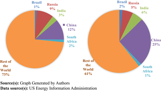
Energy has always been closely associated with economic growth and development. However, in the process the negative externalities associated with the usage of energy have not been taken care of adequately. Adverse externalities are major roadblocks to sustainable development. Climate change caused by anthropogenic global warming can undoubtedly be considered as the major hurdle to sustainable development. Left unmanaged, climate change may reverse the development progress and compromise the safety and security of present as well as future generations. According to the IPPC's fifth assessment report (AR5), the period between 1983 and 2012 has been the warmest 30-year period in the Northern Hemisphere. It is primarily caused by increased concentration of CO2, CH4 and nitrous oxide since industrialization. In fact, the concentration of CO2 in 2012 was 40% more than it was in the mid-1800s [1]. Fossil fuel and land use changes primarily cause global increase of CO2 concentration. Crude oil accounted for 39% of the world total primary energy source in 2017 and contributed to 33% of the global CO2 emissions. In 2018, CO2 emissions reached a historic high of 33.1 Gt. Nearly two-thirds of global emissions for 2011 originated from only 10 countries, with shares of China (25.4%) and the United States (16.9%) far surpassing the rest. Combined, these two countries alone produced 13.2 Gt of CO2. The two high emitter countries are followed by India, Russian Federation, Japan, Germany, Korea, Canada, Islamic Republic of Iran and Saudi Arabia. Further, by 2012, Brazil, Russia, India, China and South Africa (BRICS) countries emissions had increased to 39% of the total world emissions, from 27% in 1992. As represented in Figure 1, a quarter of the total world emissions in fact are from China alone. India presently is the third largest emitter of CO2 in the world. The emissions of Brazil and India as a percentage of total emissions in the world doubled in 2012 compared to 1992. Over the same period, Russia and South Africa's contribution to total world emissions decreased to 5 (from 9.44%) and 1% (from 1.5%), respectively, over the same period.
Globally, crude oil prices fell from 100US$ per barrel in mid-2014 to below 30US$ per barrel in early 2016. Natural gas and coal prices also fell during this period. International Monetary Fund (IMF) quantifies lower fossil fuel prices to act as a form of economic stimulus. According to World Energy Outlook (WEO, 2015), lower oil prices not only supports growth, but stimulates oil use as well. It also diminishes the case for efficiency investments for switching to alternative fuels.
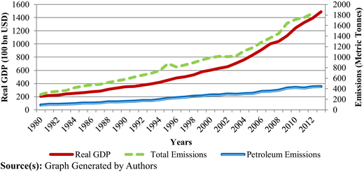
For emerging economies such as India, [2] it is important to understand how much environment friendly its economic growth is India's GDP growth rate and carbon emissions increased steadily over the period 1980–2013. India's GDP growth rate peaked at around 10% in 2010 and then slowly moved down to around 7% by 2013. In Figure 2, India's real GDP and carbon emissions from total energy consumption, as well as, from petroleum consumption for the period 1980–2013 are presented. India's real GDP witnessed a steady increase from around US $0.2tn in 1980 to around US$1.48tn in 2013. A similar increasing pattern is witnessed in carbon emissions from total energy consumption, which increased from around 291 million metric tonnes in 1980 to around 1830 million metric tonnes in 2012. Similarly, India's carbon emissions from petroleum consumption also increased from around 100 million metric tonnes in 1980 to around 435 million metric tonnes in 2012.
Government policies in developing countries are crucial in deciding the flow of foreign direct investment (FDI) to these countries. According to the UN trade body, India is the 9th largest recipient of FDI of US$52 bn in 2019. The net inflow of FDI as a percentage of GDP though is considerably small for India, it has increased from 0.02% in 1991 to 3.62% in 2008. By 2019, the net flow of FDI is at 1.76%. India's new economic policy of liberalization, privatization and globalization adopted in 1991 led to this increase in FDI inflow/outflow. However, one of the key factors influencing foreign investment in developing countries like India, is that they set environmental standards below efficiency levels. As international trade relates one country to another, developing and underdeveloped economies rely on technology transfer through FDI that may reduce pollution in the long-run (Dinda, 2004; Dean, 2004; Wheeler, 2000).
Pressure is mounting on India to commit for a legally binding agreement on cutting CO2 emissions. Under such circumstances, the need to examine the impact of various contributing factors to CO2 emissions cannot be negated. In this regard, an important element to analyze is the impact of GDP on CO2 emissions. This hypothesized inverted U-shaped relationship between environment pollutant and economic growth in economic literature is referred to as the environmental Kuznets curve (EKC).
Simon Kuznets first proposed the inverted U-shaped relationship in 1955, while explaining the relationship between income inequality and per capita income. The Kuznets curve was adapted in environmental economics literature in 1990's by economists such as Grossman and Kruger (1991), Shafik and Bandhyopadhay (1992), Panayotou (1993) and Selden and Song (1994). The EKC hypothesis summarizes a dynamic process of change – namely, as income of an economy grows over time, emission levels first grow; reach a crest and then start turning down after a threshold level of income (Y1) has been attained (Figure 3). Further, as the economy reaches income levels higher than Y2, the direction of relationship between environmental degradation and per capita income (GDP) changes. Beyond Y2, both environmental degradation and GDP move in the same direction. EKC is a long-term phenomenon and does not make an explicit reference to time. It is a development path for a single economy that grows through different stages over time. Other things remaining constant, in their process of development, each country experiences income and emission situations lying on the specific EKC. While a typical EKC is an inverted U-shaped curve, linear and N-shaped curves are also plausible.
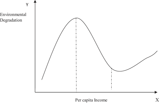
Scale effects, technological effects and composition effects are the three channels through which economic growth affects the environmental quality (Grossman and Krueger, 1991). In this initial stage of economic development, pollution increases with increasing output. As, the economy transforms from an industrial to a service economy, the pollution level plateaus. Also, with technical progress like the adaption of cleaner technologies, pollution level further reduces. Thus, scale effect that has a negative impact on the environment dominates the first stage; then with economic growth, composition effect and the technological effect that has a positive impact on the environment start dominating; thereby the inverted-U shaped curve.
International trade is a crucial factor that can explain EKC. As trade volume increases, environmental quality could decline or improve because of opposing directional impacts of scale effect, composition effect and technique effect. The composition effect is associated with two related hypotheses: displacement hypothesis and pollution haven hypothesis (PHH) (Dinda, 2004). The displacement hypothesis states that trade liberalization or openness will lead to the more rapid growth of pollution-intensive industries in less developed economies, as developed economies enforce strict environmental regulations (Harrison, 1996; Rock, 1996; Tobey, 1990; Dinda, 2004). PHH argues that with trade increasing income levels, there will be more demand for a cleaner environment, thereby pushing heavy polluting industries to countries with weaker regulations. PHH refers to the possibility of multinational firms, especially the ones engaged in highly polluting activities, relocating to countries with lower environmental protection rules and regulations. Environmental regulation exerts a moderating effect on the inverted-U shaped relationship with economic development and carbon emissions.
Since EKC is a long-run phenomenon (Lindmark, 2002), the same using time series technique is considered more appropriate (Akbostanci, 2009). As such, we use a time series methodology for the present study. In this study, we hypothesize the EKC between carbon emissions and GDP. The control variables used are, crude oil prices, trade openness, FDI inflow and select variables of economic freedom, especially as captured by size of government.
The flow of the paper is as follows: Section 2 provides the review of literature. This is followed by Section 3, where the methodology (pertaining to unit root test with structural break and ARDL technique) and data sources are discussed. Empirical results are reported in Section 4. Finally, in Section 5, the paper concludes from a broad policy perspective.
2. Review of literature
In last few decades, there has been an increasing attention on how economic growth impacts environmental degradation. Though literature documents this relationship, in general, the causal links and direction of impact remains ambiguous. While reviewing the EKC literature we begin by examining research papers that use similar econometric methodology as adopted in the present research. Thereafter, papers that adopt an alternative methodology have been reviewed. Accordingly, the next two subsections follow:
2.1 Papers based on autoregressive distributed lag (ARDL) econometric methodology
In this subsection, papers that support the EKC relationship are reviewed first, followed by papers that do not support the EKC hypothesis. Thereafter, specific papers that examine the EKC relationship for India are reviewed.
Balaguer and Cantavella (2016) perform a structural analysis on EKC for Spain for the period 1874–2011. In the research paper, real oil prices are used as an indicator of variations in fuel energy consumption. Evidence supports the EKC hypothesis in the long-run, as well as, in the short-run. Further, empirical results support the idea that changes in real oil prices are relevant in order to explain CO2 emissions. They observe that with a 1% rise in oil prices, the CO2 emissions reduce by 0.4% in Spain. They also check the possibility of flatter EKC curve in presence of technological effectiveness put forward by Dasgupta et al. (2002) and reject the same for the sample period for Spain. Boluk and Mert (2015) provide empirical evidence for the potential of renewable energy within an EKC framework for Turkey. Using ARDL approach, the relationship between carbon emissions, income and the electricity production from renewable energy sources has been investigated for the period 1961–2010. Based on their analysis, the authors conclude that there is an inverted U-shaped relationship between per capita emissions and per capita real income, supporting the EKC hypothesis in both the long and short-run. Jelbi and Youssef (2015) investigate the dynamic causal relationships between CO2 emissions, economic growth, renewable and nonrenewable energy consumption, and trade in Tunisia during the period 1980–2009. The authors observe that EKC hypothesis is not supported in the long-run, whereas in the short-run the inverted U-shaped EKC hypothesis is supported. In case of trade, both per capita exports and imports have a positive impact on per capita CO2 emissions.
The study by Ahmed and Long (2012) hypothesize EKC to investigate the relationship between CO2, energy consumption, economic growth, trade liberalization and population density in Pakistan. The study uses an ARDL model approach for a sample period from 1971 to 2009. Two main findings of the study are – first, while there is a long-run inverted U-shaped relationship between variables; there is no evidence to support the existence of EKC in the short-run. Second, trade openness improves the environment only in the short-run. Additionally, Pakistan's population density has been estimated to contribute to environmental degradation.
Tiwari et al. (2013) test the EKC hypothesis for Indian economy by incorporating coal consumption and trade openness. The study employs an ARDL model for the period 1966–2009, and reinforces the results using Johansen cointegration. Based on their analysis, the authors conclude that there is presence of EKC both in the long-run and short-run. Further, both coal consumption and trade openness also contribute to carbon emissions in the long-run. Jayanthakumaran et al. (2012) using ARDL methodology compares the relationship between growth, trade and energy use for India and China. Structural breaks are endogenously determined for the period 1971–2007 using the Lagrange multiplier unit root test proposed by Lee and Strazicich (2003, 2004). Further, existence of EKC relationship is established for both India and China. In India, the increase in energy consumption increases per capita emission by 0.97% in the long-run. However, the authors find that when manufacturing – GDP ratio is incorporated in the model, the long-run relationship between the variables no longer exists for India.
2.2 Papers based on econometric methodology, other than ARDL
For the period 1951–1986, Holtz-Eakin and Selden (1995) employ a panel data model for 130 countries. Their findings suggest evidence of diminishing marginal propensity to emit CO2 as economies develop. Further, the forecast results indicate that global emissions of CO2 will continue to grow at an annual rate of 1.8%. The study by Apergis (2016) assesses the “emission-income” relationship in EKC hypothesis using common correlated effects, fully modified ordinary least squares and the quantile estimation procedures. The analysis for 15 countries is done using data for the period 1960–2013. The results of the study indicate the presence of a nonlinear link between emissions per capita and personal income per capita across the majority of 15 countries. The paper concludes by recommending the use of more renewable sources of energy to reduce energy dependence and ensure energy security.
Using the panel data over the 1996–2012, Li et al. (2016) estimate the impact of economic development, energy consumption, trade openness and urbanization on the carbon dioxide, liquid waste and solid waste emissions for 28 Chinese provinces. The generalized method of moments estimate (GMM) estimator, as well as, ARDL estimates (long-run as well as short-run) support the EKC hypothesis for three major pollutants, namely, carbon dioxide, industrial waste water and industrial waste solid emissions in China. The results also indicate that trade openness and urbanization leads to environmental degradation in the long-run (estimates are insignificant in the short-run) in China, though the magnitude of severity varies across different pollutant emissions.
Robalion-Lopez et al. (2015) analyze various conditions for fulfillment of EKC hypothesis in the medium term for an oil-producing developing country, Venezuela. Using a model based on Kaya and Yokobori (1993), they use data from 1980 to 2010. The value of the GDP, the energy consumption and the CO2 emissions from 2011 to 2025 have also been estimated under four different scenarios which constrain GDP, productive sectoral structure, energy intensity and energy matrix. Based on the analysis, authors conclude that Venezuela does not fulfill the EKC hypothesis under any of the scenarios. The results show that Venezuela in 2010 is still in the first stage of the EKC. However, the authors state that the country could be on the way to achieve environmental stabilization in the medium term, if economic growth is accompanied with increasing use of renewable energy, appropriated changes in the energy matrix and in the productive sectoral structure.
Saidi and Hammami (2015) use a dynamic panel model to examine the impact of energy consumption and CO2 emissions on economic growth of 58 countries. The results show that energy consumption and FDI have a positive and significant impact on economic growth in the panel of countries and that CO2 emissions have a negative and statistically significant impact on economic growth. Zakaraya et al. (2015) analyze the interactions between total energy consumption, FDI, economic growth and CO2 emissions in the BRICS countries for the period 1990–2012. The major contribution in their study is the consideration of environmental pollution and the amount of carbon emissions caused by foreign investment. Their study reinforces the view that environmental policies of developing countries are incomplete. Resultantly, foreign investors who are limited by policies in their own countries, are attracted to developing economies resulting in environmental degradation.
Tutulmaz (2015) investigates the EKC relationship between CO2 emissions and GDP per capita for Turkey for the period 1968–2007. An initial phase of an inverted U-shape EKC relationship has been determined for Turkey from their estimations. Rather surprisingly, this result is conflicting with that of similar models for Turkey. Basis that, the authors title their paper as, “Environmental Kuznets Curve time series application for Turkey: Why controversial results exist for similar models?” Wang et al. (2015) provide specific application of EKC in explaining the effect of population growth on environment using overlapping generation model. Further, using data for 30 provinces from China between 2001 and 2010, effects of population growth on the population–income relationship is examined. The empirical analysis supports the presence of an inverted U-shaped relationship between polluting emissions and income. Simulation results in the paper illustrate that higher population growth makes the EKC steeper with higher peaks.
Pao and Tsai (2011) examine the dynamic relationship between CO2 emissions, energy consumption and economic growth in Brazil for the period 1980–2007. The results support the EKC hypothesis as energy–income relationship appears to be an inverted U-shaped curve. Ghosh (2010) probes the relationship between CO2 emission, energy supply and economic growth while controlling investment and employment in India for the period 1971–2006. The empirical results (using ARDL), establishes a long-run equilibrium among the variables. The results show the presence of bi-directional causality between CO2 emissions and economic growth, justifying India's stand against mandatory emissions cut by developing nations. Further, results also establish presence of unidirectional causality from economic growth to energy supply and energy supply to carbon emissions.
Cole (2004) constructs a model to examine the evidence for the PHH and to assess the extent to which trade, through pollution haven effects and structural change has contributed to the EKC relationship. Using detailed data on North–South trade flows for pollution intensive products, the evidence for the PHH is assessed. EKC analysis for six air pollutants and four water pollutants has been undertaken; and pollution haven effects have not been found to exist for all pollutants. Also, when found, their economic significance has been limited. The author also interprets that the share of manufacturing output in GDP has a positive and statistically significant relationship with pollution. Hill and Magnani (2002) too examine the EKC relationship for a panel of 156 countries using generalized least squares model. However, they find no evidence of an inverted U-shaped EKC hypothesis as emissions monotonically increase with income per capita.
List and Gallet (1999a, b) use a state-level panel data of sulfur dioxide and nitrogen oxide emissions for the period 1929–1994 for several states of America to test the appropriateness of the “one size fits all” reduced-form regression used in EKC literature. The results provide evidence to support the presence of inverted-U path. Further, the results also indicate that state-level EKC's differ from one another and over time as well, which restricts cross-sections to undergo identical experiences over time. Another observed trend is that states whose EKCs peak to the left of the traditional confidence interval tends to have higher per capita emissions of the respective pollutant presumably because states with higher per capita emissions react more quickly to adopt policies designed to reduce pollution.
To summarize, while literature on EKC is rich, the specific EKC relationship is unique to each country. Resultantly, the motivation to take up the present EKC study for India. Also, since the environment impact of India's New Economic Policy (which promotes liberalization, privatization and globalization), remains largely unexplored, the present paper analyzes the same.
3. Research methodology and data sources
The objective of the study is to verify the EKC hypothesis for India. In order to do so we examine whether the EKC follows a linear, quadratic or polynomial form. Though literature predominantly discusses quadratic form, we also examine if a cubic form EKC relationship exists between environmental pollutants and economic growth. The time period of our study is from 1980 to 2012.
In this study, to test the validity of EKC hypothesis the following equation has been estimated [3]:
Where:
EP: It represents environmental pollutant as measured by carbon emissions (CO2). In our study, carbon emissions (CO2) are from the consumption of petroleum. CO2 is in million metric tons.
Y: It represents real GDP per capita. It is the gross value of goods and services produced within the domestic territory of India in a specific period, adjusted for inflation. Real GDP divided by mid-year population provides real GDP per capita. Data are in constant 2005 US$. As represented in Eqn (1), its square and cubic form is also incorporated.
Z: It represents other variables such as trade openness, foreign direct investment, crude oil price, petroleum consumption and economic freedom as measured by Size of Government. Each of these is hereby described:
Trade openness is total value of import and exports as a percentage of GDP; FDI is net inflows as a percentage of GDP; Crude oil price is the simple average of three spot prices: Dated Brent, West Texas Intermediate and the Dubai Fateh (Base year −2005); Petroleum consumption is the total value of crude petroleum consumed. It is in thousand barrels per day and economic freedom as measured by “Size of Government”.
Among the above variables, “Size of Government” deserves a special mention. The rationale for including this explanatory variable is to understand whether countries with lower government size are more polluting. After all, theory does suggest that goods and services, which have higher social cost vis-à-vis private cost, shall be overproduced in economies that adopt more market friendly policies, necessitating government intervention. In our study, size of government is measured as per the definition and methodology adopted by Fraser Institute's Economic Freedom of the World Index. Among the five components of Economic Freedom Network Index [4] in which economic freedom is measured, size of government is one. It incorporates aspects such as government consumption, taxes and subsidies, government enterprises and investment, and top marginal tax rate. The first component, government expenditure indicates the extent to which countries rely on the political progress to allocate resources and goods and services. When government-spending increases relative to spending by individual's decision-making, its substitutes for personal choice and economic freedom is reduced. Similarly, its second component as measured by taxes also reduces the freedom of individuals to keep what they earn. The third component measures the extent to which countries use private investment and enterprises rather than government investment. Economic freedom is reduced as government enterprises produce a larger share of total output. The fourth component is based on taxes, namely, the top marginal income tax rate and the top marginal income and payroll tax rate. High marginal income tax rates are also indicative of higher government intervention. The degree to which a country relies on personal choice and markets rather than government budgets and political decision-making explains the economic freedom based on “Size of Government”. Therefore, countries with low levels of government spending as a share of the total, a smaller government enterprise sector and lower marginal tax rates earn higher ratings in terms of economic freedom as measured by “Size of Government”. It is important to appreciate that a lower size of government implies higher economic freedom as measured by this variable.
t: represents time
: constant term and coefficient parameters
e: error term
jointly determine the shape of EKC curve, i.e. a linear, inverted-U or N type EKC curve.
Mathematically
A linear relationship implies: 0 and .
An inverted U-shaped relationship implies:
A U-shaped curve implies:
A N-shaped figure or a cubic polynomial relationship implies:
The variables are briefly explained:
Data: The annual time series data for carbon emissions (CO2), economic growth (GDP), industrial development (industrialization), FDI and trade openness has been obtained from World Development Indicators (WDI) online database. Crude oil price (international price index) for the period is collected from IMF. Data for total petroleum consumption is collected from the US Energy Information Agency. Data for economic freedom variables are from Fraser Institute's Economic Freedom Index's online database.
To examine the said relationships, unit root tests with structural break, and ARDL technique has been adopted.
Unit root tests: Numerous unit root tests are available in applied economics to test the stationarity properties of the variables. The unit root tests are augmented Dickey–Fuller by Dickey and Fuller (1979), Phillips–Perron (P–P) by Phillips and Perron (1988), Ng–Perron by Ng and Perron (2001) and Kwiatkowski–Phillips–Schmidt–Shin by Kwiatkowski et al. (1992). All these do not have information about structural break points that occur in the series and hence provide biased and spurious results. Thus, in our paper, we perform a breakpoint unit root test similar to that of Perron (1989). The null hypothesis is that the time series has a unit root with possibly nonzero drift, against the alternative that the process is “trend-stationary”. For carbon emissions, the break point has been estimated in the year 1993, for both the “intercept” and “intercept and trend” model
Autoregressive distributed lag model (ARDL): Cointegration is defined as a systematic comovement among two or more macroeconomic variables over the long-run. The presence of cointegration can be considered as a pretest for possibility of “spurious” correlation among variables. A standard ARDL equation with a dependent variable, y, and two other explanatory variables, x1 and x2 will be:
where is the first difference operator.
The ARDL method of cointegration analysis was first introduced by Hendry (1995) and extended by Pesaran and Shin (1999) and Pesaran et al. (2001). An ARDL model gives a simple univariate framework for testing the existence of single level relationship between the dependent and independent variables, when it is not known with certainty whether the regressor are purely I(0) , purely I(1) or mutually cointegrated.
One of the key assumptions in the bounds testing methodology of Pesaran et al. (2001) is that the errors of Eqn (2) must be serially independent. To test for serial correlation of the residuals the Q-stat correlogram test is performed. Since we have a model with autoregressive structure we have to be sure that the model is “dynamically stable”. To test for the stability of the long-run relationship over time, the cumulative sum of recursive residuals (CUSUM) [5] test is utilized. This stability test is appropriate in time series data, especially when we do not know when structural change might happen.
After estimating regression Eqn (2), the Wald test can be carried out by imposing restrictions on the estimated long-run coefficients. The null and alternative hypotheses herein are as follows:
(No long-run relationship exists).
(A long-run relationship exists).
The computed F-statistic value is evaluated with the critical values tabulated in Pesaran et al. (2001). Pesaran et al. (2001) supply bounds on the critical values of the asymptotic distribution of the F-statistic. They give lower and upper bound critical values for various situations (different number of variables, (k+1)). In each case, the lower bound is based on the assumption that all the variables are I(0), and the upper bound is based on the assumption that all of the variables are I(1). If the computed F-statistic falls below the lower bound one concludes that the variables are I(0), so no cointegration is possible. If the F-statistic exceeds the upper bound, it is concluded that cointegration exists. Finally, if the computed F-statistic falls between the lower and upper bound values, then the results are inconclusive. Further, if there is evidence of long-run relationship (cointegration) among the variables, ARDL-EC model is used to estimate the long-run relationship and also to estimate the short-run dynamics.
4. Empirical results
4.1 Unit root test
To ensure that none of the variables are stationary at I (2) or beyond that order of integration, breakpoint unit root test has been conducted. All variables have been tested at level and at first differences. Table 1 reports the results of the breakpoint unit root tests with “intercept” and “intercept and trend”. It shows that all variables are stationary at I (0) or I (1).
Breakpoint unit root test
| Intercept (t statistic) | Intercept and trend (t statistic) | |||
|---|---|---|---|---|
| Level | 1st difference | Level | 1st difference | |
| CO2 | −1.28 | −7.06*** | −6.37*** | |
| GDP | 1.45 | −5.41*** | −3.35 | −6.64*** |
| GDP2 | 4.32* | −2.16 | −7.97*** | |
| GDP3 | −1.97 | −3.82 | −3.68 | −7.65*** |
| Oil price | −3.15 | −7.36*** | −4.69** | |
| Petroleum consumption | −1.38 | −6.34*** | −2.94 | −6.65*** |
| Trade openness | −1.36 | −6.93*** | −5.47*** | |
| FDI | −3.53 | −6.75*** | −3.52 | −6.85*** |
| Size of government | −5.90*** | −6.84*** | ||
Note(s): ***, ** and * denote level of significance at 1, 5 and 10%, respectively
4.2 ARDL
Thereafter, the ARDL bound testing approach has been applied to examine the long-run relationship between variables. The advantage of bound testing is that it is flexible regarding the order of integration of the series[6]. Following the Schwarz criteria (SC), a lag length of 2 was chosen, for all models. The structural break of CO2 emissions series estimated at year 1993 is taken across all model specifications.
The aim of the present study is to investigate the relationship between environmental pollutant (as measured by CO2 emissions) and GDP for India. Following the methodology as developed by Jebli and Youssef (2015) and Jayanthakumaran et al. (2012), among others, we develop two models based on EKC hypothesis: Model 1 and Model 2 [7].
The general empirical form of Model 1 is:
Model 1 can be rewritten as an ARDL model with intercept and trend as follows:
Model 2 is an extension of Model 1 and includes two more explanatory variables, namely, size of government and FDI.
Table 2 reports the results of ARDL bounds testing approach to cointegration in the presence of a structural break in the series. The results show that our calculated F-statistics is greater than upper bound at 1 and 10% levels in models 1 and 2, respectively. This leads us to reject the null hypothesis of no cointegration. This indicates that there is a cointegrating relationship among the variables across models in the long-run. Q-stat for Model 1 and Model 2 are provided in Tables A1 and A2.
Bounds testing for cointegration
| F-statistics | With a time trend | ||
|---|---|---|---|
| Model 1 | CO2 and GDPPC, crude price, petroleum consumption, trade openness | 8.97*** | |
| *F-critical at 1% level1 k (6) | I(0) | I(1) | |
| 3.60 | 4.90 | ||
| Model 2 | CO2 and GDPPC, crude price, petroleum consumption, trade openness, FDI, size of government | 3.68* | |
| *F-critical at 10 % level2 k (8) | I(0) | I(1) | |
| 2.26 | 3.34 | ||
Note(s): ***, ** and * indicates level of significance at 1, 5 and 10%, respectively
Q-stat for Model 1
| Q-statistic probabilities adjusted for 1 dynamic regressor | ||||||
|---|---|---|---|---|---|---|
| Autocorrelation | Partial correlation | AC | PAC | Q-stat | Prob* | |
| | .…| | | .…| | 1 | 0.013 | 0.013 | 0.0064 | 0.936 |
| | .…| | | .…| | 2 | 0.015 | 0.015 | 0.0150 | 0.993 |
| |* .…| | |* .…| | 3 | 0.091 | 0.090 | 0.3309 | 0.954 |
| | .…| | | .…| | 4 | −0.018 | −0.021 | 0.3436 | 0.987 |
| *| .…| | *| .…| | 5 | −0.153 | −0.157 | 1.3130 | 0.934 |
| *| .…| | *| .…| | 6 | −0.118 | −0.126 | 1.9123 | 0.928 |
| **| .…| | **| .…| | 7 | −0.294 | −0.298 | 5.7483 | 0.569 |
| *| .…| | *| .…| | 8 | −0.149 | −0.151 | 6.7759 | 0.561 |
| **| .…| | **| .…| | 9 | −0.268 | −0.313 | 10.222 | 0.333 |
| | .…| | | .…| | 10 | 0.060 | 0.032 | 10.402 | 0.406 |
Note(s): *Probabilities may not be valid for this equation specification
Q-stat for Model 2
| Q-statistic probabilities adjusted for 1 dynamic regressor | ||||||
|---|---|---|---|---|---|---|
| Autocorrelation | Partial correlation | AC | PAC | Q-Stat | Prob* | |
| *| .…| | *| .…| | 1 | −0.107 | −0.107 | 0.4016 | 0.526 |
| **| .…| | **| .…| | 2 | −0.228 | −0.242 | 2.2873 | 0.319 |
| *| .…| | *| .…| | 3 | −0.080 | −0.147 | 2.5283 | 0.470 |
| *| .…| | **| .…| | 4 | −0.191 | −0.308 | 3.9500 | 0.413 |
| |* .…| | | .…| | 5 | 0.106 | −0.050 | 4.3987 | 0.494 |
| | .…| | **| .…| | 6 | −0.060 | −0.241 | 4.5484 | 0.603 |
| | .…| | | .…| | 7 | 0.058 | −0.057 | 4.6964 | 0.697 |
| | .…| | **| .…| | 8 | −0.028 | −0.211 | 4.7309 | 0.786 |
| |* .…| | |* .…| | 9 | 0.185 | 0.175 | 6.3581 | 0.704 |
| *| .…| | *| .…| | 10 | −0.069 | −0.165 | 6.5938 | 0.763 |
| **| .…| | **| .…| | 11 | −0.278 | −0.235 | 10.608 | 0.477 |
| | .…| | .**| .…| | 12 | 0.000 | −0.268 | 10.608 | 0.563 |
| | .…| | **| .…| | 13 | −0.005 | −0.226 | 10.610 | 0.643 |
| |**. | | *| .…| | 14 | 0.263 | −0.068 | 14.783 | 0.393 |
| |* .…| | | .…| | 15 | 0.134 | 0.011 | 15.931 | 0.387 |
| *| .…| | **| .…| | 16 | −0.192 | −0.248 | 18.442 | 0.299 |
Note(s): *Probabilities may not be valid for this equation specification
As for the expected sign of explanatory variables other than, and (estimated coefficients of GDPPC, GDPPC2 and GDPPC3, respectively), one expects the coefficient of crude oil price to be negative since an increase in price of oil is expected to reduce oil consumption. Further, the coefficient for petroleum consumption is expected to be positive, as higher consumption is expected to promote pollution. The coefficients of trade openness and FDI may be positive or negative depending upon the level of economic development. In general, if developing economies have less stringent environment regulations, greater trade openness and more FDI are expected to increase pollution. Finally, coefficient of economic freedom index as measured by “Lower Size of Government” is expected to be positive as economies with greater private sector participation may overproduce goods and services for which social costs outweigh private costs. This certainly is the case with pollution emitting industries where negative externalities are immense.
The results of cointegration tests are reported in Table 3. We proceed with a cubic form for EKC hypothesis for both the models.
Estimation of EKC models for India
| Variables | Model 1 | Model 2 | ||
|---|---|---|---|---|
| Long-run | Short-run | Long-run | Short-run | |
| GDPPC | 0.0011*** (0.0003) | 0.0027*** (0.0005) | 0.3823*** (4.1419) | 2.5047*** (4.6648) |
| GDPPC2 | −0.0000 (0.0000) | −0.0000**** (0.0000) | 0.0001** (2.3727) | −0.0044*** (-4.8145) |
| GDPPC3 | −0.0000*** (0.0000) | 0.0000*** (0.0000) | −0.0000*** (−7.1727) | 0.0000*** (4.8327) |
| Crude oil price | −0.0015** (0.0005) | −0.0009*** (0.0002) | −0.1178** (−2.9326) | −0.3190*** (−3.2847) |
| Petroleum consumption | −0.0000 (0.0000) | 0.0001** (0.0000) | 0.07482*** (13.2693) | 0.0707*** (6.1319) |
| Trade openness | 0.0057** (0.0024) | 0.0008 (0.0012) | −1.5929*** (−8.3154) | −36.3374*** (−14.0013) |
| FDI | 5.5617*** (5.9571) | −11.5328*** (−4.3841) | ||
| Size of government | 10.2671*** (14.1573) | 27.7889*** (14.0115) | ||
| Break1993 | −0.0057 (0.0053) | −0.0062 (0.0054) | 23.9877*** (11.3482) | 64.9250*** (9.4844) |
| Trend | −0.0099** (0.0031) | −0.0108*** (0.0027) | −2.2457*** (−3.8060) | −6.07817*** (−4.3306) |
| Constant (C) | −0.1404* (0.0715) | −92.0408*** (−4.4271) | ||
| Error correction term | −1.0872*** (0.1539) | −2.7066*** (−15.3902) | ||
| R2 | 0.9972 | 0.9997 | ||
| DW | 2.3409 | 2.2051 | ||
Note(s): ***, ** and * denote level of significance at 1, 5 and 10%, respectively. Figures in parenthesis represent standard errors
In models 1 and 2 [8], the coefficient of GDPPC remains positive and significant across specifications. For Model 1, the coefficient of GDPPC square and GDPPC cube equals zero implying that there is a monotonic increase in carbon emissions with an increase in per capita GDP. This largely implies that EKC's linear model hypothesis (and not inverted U-shaped hypothesis) is valid for India both in the long-run and short-run. However, in Model 2, in the short-run, presence of an inverted U-shaped EKC has been estimated. Further, as expected, increase in crude oil price has a negative and significant effect on carbon emissions, as the estimated coefficient is negative (and significant) across model specifications. Also, where significant, the coefficient of petroleum consumption is positive. This implies that higher consumption of energy is associated with increase in carbon emissions. This result is also as per expectation. In Model 1, the coefficient of trade openness is positive and significant at 5% level in the long-run. This implies that increase in trade openness is expected to be linked with higher carbon emissions in the long-run. However, in Model 2, the coefficient of trade openness is negative and significant at 1% level, both in the long-run and short-run.
Further, in Model 2, the coefficient of FDI is positive and significant at 1% level in the long-run but negative and significant in the short-run. This implies that an increase in FDI is expected to be linked directly with carbon emissions in the long-run, but not in the short-run. In Model 2, the coefficient of economic freedom as measured by lower “size of government” is positive and significant. This means that periods during which size of government is lower are associated with higher carbon emissions. In Model 2, the coefficient of trade openness and size of government in the short-term corroborates with the long-term relationship established.
In the short-run as expected, the coefficient of the error correction terms is negative and significant across model specification (at 1% level). This corroborates with our established long-run relationship between carbon emissions, GDPPC and other variables. The changes in carbon emissions are expected to be corrected within a year. Further, it is expected that full convergence will take place within a year and reach the stable path of equilibrium. Thus, we may conclude that the adjustment process is fast for the Indian economy.
5. Conclusion and policy recommendations
Based on the hypothesis of EKC, the study investigates the relationship between environmental pollutants (as measured by CO2 emissions) and per capita GDP for India, over the period 1980–2012. Making use of the ARDL bounds testing approach for cointegration with structural breaks, the presence of EKC has been examined (in two model specifications: both long-run and short-run) while controlling for factors such as oil prices, petroleum consumption and trade openness in Model 1, as also, FDI and size of government in Model 2.
The main findings of the study are:
A monotonic relationship is observed between per capita carbon emissions and per capita GDP in Model 1, both in the long-run and short-run. Evidence to support existence of an inverted “U” shaped EKC, in India is validated only in the short-run for Model specification 2. This implies that carbon emissions begin to decline, once the threshold level of GDP per capita is achieved.
Rise in fuel price leads to reduction in carbon emissions and increase in petroleum consumption promotes emissions.
Impact of trade openness is ambiguous across model specifications. While in Model 1, the long-run impact of trade openness induces carbon emissions,in model 2, increase in trade is associated with lower levels of carbon emissions. The short-run impact of trade openness in Model 2 is negative (and significant) implying that as the Indian economy opened to trade, in the short-run, the CO2 emissions reduced.This can be on account of technological and composition effects that are expected with economic growth and FDI inflow in an open economy.
In Model 2, an increase in net FDI inflow has an adverse effect on environment in the long-run, though the short-run impacts on environment are favorable. Some of these findings are in line with those of Pao and Tsai (2011), Jian and Rencheng (2007) and Havens (1999), as they too have estimated that higher FDI increases environmental degradation. This indicates that India (like other developing countries) attracts FDI in polluting industries, maybe because of lower environmental standards. This incentivizes heavy polluters to move to countries with lower environment regulations. The migration or displacement of “dirty” industries from the developed regions to the developing regions is referred to as “Pollution Haven Hypothesis (PHH)”. The PHH theory of polluting multinational companies coming to countries with lower environmental standards is supported by our results. In addition, the environmental quality could decline through the scale effect as increasing FDI/trade volume raises the size of economy, which per se increases pollution as well.
Our findings indicate that higher economic freedom as measured by lower size of government has a positive impact on carbon emissions. Adverse impact of lower size of government on environment is in sync with the theory of negative externalities as proposed by Stiglitz. This relationship validates the theory that greater participation by the private sector in economic activities of a nation, promotes negative externalities such as those caused by smoke or air pollution. To address concerns of market failure, governments must introduce effective regulations to address climate concerns.
Based on our findings, important policy recommendations are hereby proposed:
Adopting interventionist policies to control environmental degradation: Several studies (Tiwari et al., 2013; Jayanthakumaran et al., 2012; Agras and Chapman, 1999; Sajeev, 2018) have shown that one may expect a delinking between environmental degradation and economic growth beyond the threshold limit, as and when it is attained. In such cases, promotion of economic growth seems to be a sufficient condition for safeguarding environment. However, our finding suggests that growth and carbon emissions go together. Since economic growth cannot be compromised, especially for developing economies such as India, governments need to actively introduce interventionist policies to control environmental degradation.
Rationalizing and phasing of government fossil fuel subsidies: According to the IEA statistics, oil subsidies in India were 29.7bnUS$ in 2014 (Real, 2013). For the same period, China's oil subsidies stood at 11.8bn US$. Such high subsidies need to be reduced and rationalized. IEA reports that removing fossil fuel subsidy can limit carbon emissions by 2.6Gt by 2035, which is nearly half of the reduction needed to limit global warming to 2°C. While the main aim for subsidy is to make it more affordable, especially for the poor and vulnerable, often the impacts are not optimal due to poor targeting and/or associated systemic leakages. Since subsidies reduce the incentive to curb wasteful energy consumption, there is an associated environment cost of subsidy as well. Straining of government budgets in such cases also reduces government's flexibility to invest in greener technologies. To mitigate the adverse social consequences of removal of fossil fuel subsidies, cross-subsidization can be introduced for promoting use of renewable energy sources, as also more energy efficient technologies.
Imposition of carbon tax: The explicit costs of carbon emissions, in general, are paid by the public in the form of rising health care costs and higher food prices due to crop failures. Stern Review (2006) suggests that climate change is a classic example of market failure. By introducing carbon tax, governments can reduce the gap between private and social cost of fossil fuel consumption. This shall promote more efficient usage and utilization of the fuel as carbon tax increases the price that consumers pay for energy. IMF proposes a global carbon tax at $75 per tonne of carbon to help limit global warming to 2°C above preindustrial levels. The IMF estimates that a carbon tax of $75 per tonne of carbon consumed in India will increase the price of coal by 230%, natural gas by 25%, electricity by 83% and petrol by 13%. Fortunately, the current fall in oil prices have presented an opportunity to emerging economies to introduce a flexible regime of carbon taxing that can be linked with crude oil prices. Removal of fossil fuel subsidy and carbon taxation should be integrated with clean energy and energy savings scheme derived from technology transfers that are aimed under the Kyoto Protocol. Usage of renewable energy sources is to be promoted as well for energy secure future.
To conclude, reinforced by India's stance on promoting liberalization, privatization and globalization, effective environment friendly regulatory mechanisms must be in place.
Notes
International Energy Agency Report, 2015, Outlook-India report. International Energy Agency.
Fastest growing economy in 2018 with a growth rate of 7.3%, ADB.
Economic freedom of the world measures the degree to which the policies and institutions of the countries are supportive to economic freedom.
CUSUM test and the cumulative sum of squares of recursive residuals (CUSUMSQ) test was proposed by Brown et al. (1975). The null hypothesis is that the coefficient vector is the same in every period and the alternative hypothesis is that they are different. The CUMSUM and CUSUMSQ statistics are plotted against their 5% critical bound. If the plot of these statistics remains within the critical bound, one fails to reject the null hypothesis of no structural change.
The variables can be integrated of the order I(0) or I(1) or I(0)/I(1).
Only the Models that are stable and without autocorrelation are reported in the study.
Model 1, controls for trade as a factor influencing EKC, whereas in Model 2, FDI and size of government along with trade and other variables are considered. Thereby, contributing to the differences in results of EKC between Models 1 and 2. In Model 2, both in the long- and short-run an increase in volume of trade is associated with lower levels of carbon emissions. This can be attributed to technological and composition effects on account of economic growth and FDI.

