


Integral bridges are common structures due to their robust structural system and good durability characteristics. The structural behaviour of an integral bridge links together the superstructure, substructure and embankment soil. However, it is not clear what the resulting stiffness of the embankment soil is when the bridge superstructure undergoes daily and seasonal changes in its length, which cause cyclic translational displacements of the bridge ends with stub-type end screens that might be uneven. Using the ‘integral bridge simulator’, an experimental campaign was conducted to study the behaviour with a single soil material under different compaction ratios. The results of the study indicated that soil behaviour is sensitive to the compaction ratio, which suggests that the compaction ratio may be a contributing factor to the uneven displacements of integral bridge ends from thermal loads. A comparison of empirical design models revealed that the resulting displacement–pressure curve is associated with two factors – the displacement required to mobilise a certain ratio of passive earth pressure and the actual value of the passive earth pressure. The latter in particular varies with the compaction ratio of the soil.
Notation
- Ahys
area under hysteresis loop
- B
width of loading plate
- C
stiffness parameter of soil
- c
cohesion of soil
- d
movement of loading plate or bridge end screen
- drange
movement range from most contracted to most expanded state of bridge end
- dtot
total movement of loading unit
- du
wall movement when KP is reached
- d50
wall movement when 50% of KP is reached
- Eur
reference elastic modulus of soil during unloading and reloading
- E50
reference stiffness modulus of soil in hardening soil model
- F
applied force
- H
height from top of soil to bottom of loading plate
- h
height of loading plate
- Kmob
mobilised earth pressure coefficient
- KP
passive earth pressure coefficient
- K0
earth pressure coefficient at rest
- K50
earth pressure coefficient at 50% of KP
- kCR
compression modulus of cellular rubber (CR) layer
- kre
modulus of lateral subgrade reaction during reloading of minor cycle in test
- ktot
resulting lateral modulus of subgrade reaction
- m
soil stress exponent
- pav
average earth pressure along area of loading plate or bridge end screen
- Rf
factor that enables the hyperbolic equation to reach a final value instead of a near-asymptotic value
- r
wall friction
- w
water content of soil
- z
depth coordinate of soil in tests or in bridge approach embankment soil
- αp
stiffness parameter of soil
- γs
measured dry density of soil
- △H
distance between top of soil to top of loading plate
- ϕ
friction angle of soil
1. Introduction
1.1 General
The integral bridge is a common bridge type due to the structural benefits it provides compared with conventional abutment bridges. This has been acknowledged by many researchers, including White et al. (2010). When compared with conventional abutment bridges, integral bridges can often be built using a smaller amount of construction materials and with a shorter building time (Laaksonen, 2011; Maruri and Petro, 2005). Integral bridges also have the advantage of eliminating the need for costly maintenance of expansion joints, which can contribute to significant costs over the bridge's lifespan (Burke, 1988; Horvart, 2005; Kerokoski, 2005; Pétursson, 2015). Integral bridges are also known for their good resistance during earthquake events (Erhan and Dicleli, 2014).
However, although integral bridges are prevalent, the design models that account for soil–structure interaction (SSI) at bridge ends vary between countries and regions. One recognised uncertainty in these models is the complex SSI under cyclic loading (Huntley and Valsangkar, 2013; Tabatabai et al., 2017; White et al., 2010). The restrained effects between the superstructure, substructure and the movement of bridge ends primarily due to thermal load are essential characteristics of integral bridges. The temperature variations of bridge superstructures have been studied by several researchers (e.g. Arsoy, 2008; Vill et al., 2021). One explanation for the limitation of the maximum length of an integral bridge is the limited embankment soil deformations at the bridge ends. Movement of the end screen of an integral bridge towards the embankment leads to the generation of significant reaction forces from the soil against it. Consequently, the embankment soil exerts a substantial influence on the longitudinal stiffness of an integral bridge and significantly impacts the displacements of bridge ends due to thermal loads.
Based on bridge monitoring, researchers have concluded that the movements of integral bridge ends are unequal between supports (Barker and Carder, 2000; Darley et al., 1998; Laaksonen, 2011). One proposed reason for this unequal movement is strain ratcheting in the embankment soil (England and Tsang, 2005). Another suggestion is that the uneven movements may be due to SSI and uncertainties related to soil properties. However, the factors that cause these unequal movements remain unclear.
1.2 Scope of this study
In this study, experimental research on the behaviour of soil was conducted in the context of stub-type end screens under conditions of cyclic transversal movement, with the soil compaction ratio being a variable. The findings of the experimental study were compared with design models and the parameters of these models were subsequently fitted to the results.
A comparison of the results with long-term monitoring results of a typical integral bridge in Finnish conditions (Haavistonjoki Bridge) was also carried out. Detailed discussions of the bridge’s structure and analysis can be found elsewhere (Kerokoski, 2006; Laaksonen, 2004, 2011). An additional objective of this study was to demonstrate the effect of the elastic layer on the SSI of the end screen and embankment soil. Numerical modelling was beyond the scope of this study, as was the behaviour of the bridge under seismic or dynamic events.
1.3 Literature review
Test devices and test series to measure passive earth pressures have been conducted in several studies. One early experimental study with a wide scope was conducted by Rowe and Peaker (1965). In that study, the relationship between wall displacement and passive earth pressure was studied for the case of fine sand. A monotonic loading history was applied and it was observed that the soil strength and stiffness were significantly influenced by the compaction ratio of the soil. When the ratio between lateral movement and the height of the loading plate (d/H) was 5.6%, the earth pressure was two times higher with dense sand, and the friction angle (ϕ = 39°) was higher than that for loose sand (ϕ = 33). The passive earth pressure coefficient (KP) was 4.5 for loose sand, while it was 7.5 for dense sand before the wall friction (r) was exceeded on the surface of the loading plate.
The mobilised earth pressure (Kmob) of a wall structure with transversal displacement at the top (rotational displacement mode of the wall) was studied in full-scale tests by Vogt (1983). No significant difference was obtained between the values of Kmob under monotonic and cyclic loading, and it was found that Kmob could be approximated as:
Thus, Kmob is a function of the depth coordinate z and the transversal movement d. The model includes the classical coefficients of the earth pressure at rest K0 and the passive earth pressure coefficient KP. It was defined that the stiffness parameter of the soil (αp) multiplied by z should match the displacement when 50% of passive earth pressure (K50) is mobilised (Vogt, 1983). It can be concluded that the soil properties and compaction ratio can be accounted for by means of the stiffness parameter αp. The Vogt model is applied in German guidelines for bridge design (BDV, 2022). For compacted soil, the proposed values for αp are in the range 0.01–0.03 (BDV, 2022; Vogt, 1983); for loose soil, αp = 0.11 provides a good match (Laumans, 1977). The αp values mean that K50 is reached at a displacement d50, which is equal to 0.2–0.8% of the abutment height H. It needs to be emphasised that the end part of Equation 1 is hyperbolic, and then it has asymptotic value. A failure ratio (Rf) was proposed for the hyperbolic failure criterion by Duncan and Chang (1970), with Rf being the ratio between the values of the asymptotic and failure. Using Rf, the failure value can be determined. Duncan and Chang (1970) proposed Rf = 0.75 – 1.00.
Similarly to Laumans (1977) and Schmidt (1981), Vogt (1983) concluded that, with small movements, the same degree of Kmob is achieved along the depth z. With an increase in movement, soil friction is reached first near the top surface.
The Austrian guideline (Önorm, 1993) gives Equation 2 for Kmob in the case of rigid abutment transversal movements:
Equation 2 includes the whole range of displacements (drange) from the most contracted to the most expanded state of the superstructure at the top part of the wall. It seems that strain ratcheting is considered because of the application of drange in the equation. According to Equation 2, in the case of a rigid abutment, K50 is reached when d50 equals 1% of H.
Fang et al. (1994) developed a testing apparatus in which the loading plate can be driven by translational movement or by rotational movement due to a varying centre of rotation on the top or bottom of the loading plate. In that study, monotonic loading was applied and sand with a single compaction ratio was used. Fang et al. (1994) concluded that, with translational wall movement, the pressure distribution was essentially hydrostatic. The friction angle of the soil was ϕ = 31° and the resulting value of KP was 5.5. The results were in good agreement with the findings of Rowe and Peaker (1965). The results for the case of the centre of rotation at the bottom of the plate yielded experimental data such as the pressure distribution of the frame type of integral bridges. This test device was advanced because the loading plate was driven by a variable-speed motor and driving rods, and lubrication layers were placed next to the side walls to prevent friction in order to obtain two-dimensional results from the tests.
Full-scale passive loading tests on site were conducted and reported by Thompson and Lutenegger (1998) and Thompson (1999). The width B of the test wall was 2.44 m and the height H was 4.57 m. The centre of rotation for the test was on the base of the wall. The test arrangement included three wing-wall orientations of 0°, 45° and 90° with respect to the wall. The tests were conducted using one granular soil with one target density. The results indicated that the wing-wall orientation had a significant effect on stiffness because wing walls confine the backfill soil. The relative degree of compaction compared with a Proctor compaction test (RD) was on average 91%, but varied from 85% to 93% between filling layers. The results also showed large variations in Kmob at different depths. Bozorgzadeh (2007) conducted full-scale tests, and emphasised that soil properties must be carefully determined and that the level of compaction had a significant effect on the stiffness of the embankment soil.
The full-scale tests conducted by England et al. (2000) demonstrated the effects of cyclic loading. The strain ratcheting effect was observed in this study. In contrast to the tests conducted by Vogt (1983), which involved gradually increasing movement, the tests were initiated with the application of maximum displacement. The model accounted for both loose and dense sands, as well as the effect of the compaction ratio. The displacement d50 varied between 4% and 1% of the abutment height H for loose and dense sand, respectively. The effect of compaction indirectly accounted for the ratcheting effect because it provides a range of earth pressures along displacements for bridge design.
Full-scale passive loading tests with one-way increasing load cycles were reported by Lemnitzer et al. (2009). They reported KP = 16, with soil friction angle ϕ = 40° and soil cohesion c = 14 kN/m2, while the r value in the tests was in the range of 1/3ϕ–1/2ϕ.
In the Swiss (Astra, 2011) and British guidelines (BSI, 2011), Equation 3 is provided for Kmob in the case of rigid abutment transversal movements:
The proposed value for the stiffness parameter C of the soil is 40 (Astra, 2011; BSI, 2011), meaning that K50 is reached when d50 is 0.4% of the abutment height H. Both guidelines also include a method that accounts for the effects of annual cyclic loading, which is done by giving the range of Kmob that needs to be considered along the cyclic movement range. Most probably, the model was based on the research conducted by England et al. (2000).
According to the Finnish guidelines (FTA, 2021), KP is reached through displacement du equal to 1.5% of H. In addition, K50 is reached at displacement d50 = du/4, which equals 0.38% of H. The linear interpolation between the previous points is provided in the guidelines. KP is set as a constant value of 8.0 and the soil friction angle is assumed to be 38°. Strain ratcheting is accounted for by considering equal Kmob in a certain displacement range. The range is given by shifting the Kmob–d output of the monotonic case towards the contracted side. The resulting output is rather similar to that given in the British guidelines (BSI, 2011).
A recent experimental campaign was conducted by Alqarawi et al. (2024). In that work, H = 1.1 m and movement was applied monotonically or cyclically, in addition to large movements away from the backfill. The used soil in tests was black sand with a friction angle of 31° and a density target of medium–dense. The resulting earth pressures exceeded the assumed earth pressure level based on the British guidelines (BSI, 2011). The effect of the elastic layer was also tested by applying an expanded polystyrene layer between the loading plate and the backfill, which decreased backfill deformations by up to 60%.
It can be concluded from this literature review that there is need for experimental validation of the design models. This is particularly evident in the case of a shallow stub-type end screen of an integral abutment bridge, where movement resulting from thermal load is predominantly transversal and does not involve significant rotation. The sensitivity of soil behaviour to varying compaction ratios is also not yet fully understood, so additional information would be beneficial when updating the design models.
The literature shows that it is common practice in bridge design to derive the stiffness properties of the soil using with relatively straightforward methods with simple soil parameters. KP is derived and the displacement required to achieve KP, or part of it, is assessed. The required displacement is often assumed to be related to the height of the structure. In the case of a stub-type integral bridge, this relationship is to the H of the end screen. It can also be concluded that the movement (d ) needed to mobilise earth pressure is larger in loose soils than in dense soils. It appears that strain ratcheting is considered in some models directly, while some models include it but it is not mentioned explicitly.
If the soil properties of an embankment differ, eccentric displacement of the bridge abutments may occur when thermal loading causes larger movement toward the less compacted embankment. It is necessary to study how the elastic layer would affect this behaviour.
2. Test configuration of the integral bridge simulator (IBS)
2.1 Assembly
To study the interaction between the end screens and the embankment of an integral bridge, a test apparatus called the IBS was constructed (Mäntyranta, 2011, 2015). Instead of full-height abutment walls, the scope of the simulator covers shallow stub-type end screen structures. The IBS has also made it possible to test the effects of the incorporation of a flexible material (Tuominen, 2008) between the end screen and the embankment to reduce the stresses and uneven displacement of the bridge ends.
The obvious advantage of the test setup is that results can be obtained much more quickly than collecting data from existing bridges. In addition, the compaction levels can be obtained with greater accuracy. On-site measurements also introduce unknown factors due to long-term settlement of the embankment soil from causes other than the actual SSI.
The IBS consists of two opposite loading plates and soil containers filled with soil material that is been compacted. The soil in the containers represents the soil of the bridge embankment. A cross-sectional view and dimensions of the IBS are shown in Figure 1.
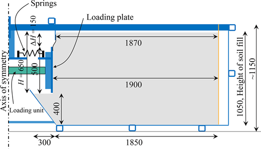
The movements of the loading plates and the reaction force are generated by a displacement-controlled step motor. The loading plates interact with each other like the actual end screens of an integral bridge through the bridge superstructure. The system allows the loading plates to have different movements, representing unequal movements of the bridge ends. The movements of the loading plates are horizontal without significant rotation because they have translational movement along the steel guides on both sides of the IBS. A small rotation (≈0.015 rad at the highest load) was generated during the highest loads due to deformation of the steel frame of the IBS.
Force was applied to the centre of the loading plates (h × B = 0.5 × 1.2 m). The height from the top of the soil to the bottom of the loading plate (H ) was 0.65 m. Hence, the distance between the top of the soil and the top of the loading plate (ΔH ) was 0.15 m. Plaster-coated plywood panels (PCPPs) were mounted on the loading plates to imitate contact between the concrete of the screen and the embankment backfill soil. Tests with cellular rubber (CR) were also conducted to study the effects of a flexible material between the bridge end screen and the embankment. The dimensions of the soil fill in the containers were 1.2 m wide (the same as B), 1.05 m high and 1.9 m long.
A photograph of the IBS is shown in Figure 2, with the locations of the loading plates inside the soil containers highlighted. The loading plates are guided by linear bearings and steel guides outside of the containers.
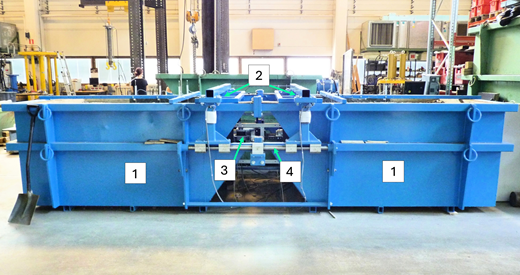
The IBS: 1, soil container; 2, loading plates; 3, loading unit; 4, sliding guides for loading plates
The IBS: 1, soil container; 2, loading plates; 3, loading unit; 4, sliding guides for loading plates
The side walls of the soil containers near the loading plates were built using plywood splices covered with a flexible material (Figure 3(a)). The side wall was designed as a flexible structure to minimise friction between the soil material and the side walls. This was achieved by allowing the side walls to compress along with the displacement of the soil material to form near a half-space boundary.
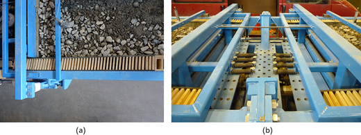
(a) Structure of side walls in soil containers of the IBS. (b) Springs between the frame of the test device and the loading plates
(a) Structure of side walls in soil containers of the IBS. (b) Springs between the frame of the test device and the loading plates
Springs were added between each loading plate and the steel frame of the device (Figure 3(b)). The steel frame is attached to the walls of the containers and then to the test floor. This was implemented to avoid a situation where the rig of the loading plates and the step motor could freely move along steel guides; for example, one loading plate would undergo almost all movements (the container with the looser soil) while the other plate (the container with the stiffer soil) would undergo very small movements.
The stiffness of the springs was set so that they represented a lower bound of the stiffness of the structures of real integral bridges with relatively flexible supports. The total stiffness of the springs per loading plate was set to 0.12 kN/mm (Mäntyranta, 2011). The elastic springs were relatively loose because they simulate the longitudinal stiffness of bridge piers, and they are often relatively slender in road bridges – at least in Finnish practice. In this way, the apparatus allows unequal displacements of the loading plates between the containers but does not lead to unrealistic behaviour of the system with very large movements on one loading plate.
2.2 Measured values
The measurement set of the IBS includes:
the horizontal movements of the loading plates
the horizontal force
the vertical position of the resultant of the passive earth pressure
the friction force between the soil and the loading plates
the settlements at the top of the soil fill
the longitudinal strain in the soil.
The applied force in the tests was measured with a load cell installed next to the loading unit. The resultant force of the earth pressure and the force produced by the loading system are equal when the force caused by the stretching of the springs is subtracted from the loading force. Transversal movements of the loading plates were measured at each corner of the plates by means of displacement gauges. The settlements at the top of the soil fill were measured at four locations on both soil containers.
2.3 Loading curves
The loading plates were displacement-controlled during the tests. The loading rate was affected by the desired loading time and range of total displacement. The tests included a cyclic displacement history, single loading and failure loading. The cyclic displacement history was used to simulate annual changes of the bridge length caused by temperature fluctuations. The cyclic displacement history followed a double sine curve with the horizontal axis representing time and the vertical axis representing the total displacement of the plates. One main cycle of the displacement history represented the range of one annual thermal displacement curve. Short-term changes in thermal displacements were taken into account by combining a 17-fold higher frequency sine curve to the annual thermal displacements (Figure 4).
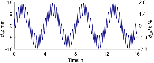
The total amplitude of the combined annual and short-term displacement curves was 17.5 mm. The amplitude is the total displacement of the loading unit (dtot), which represents the expansion and contraction of the bridge superstructure. The amplitude of a minor cycle was set to 5 mm. The amplitudes and frequency were estimated based on observations of the monitoring of bridges by Laaksonen (2011). The appropriate loading rate was tested by performing the main cycle for 4 h, 24 h and 72 h. The results from the tests were practically identical and therefore 4 h per main cycle was considered suitable for the actual test series (Mäntyranta, 2015).
3. IBS tests and bridge monitoring
3.1 Haavistonjoki Bridge
Details and results of the monitoring of Haavistonjoki Bridge between 10 October 2003 and 10 October 2010 have been presented in several publications, mainly those of Laaksonen (2004, 2011, 2023) and Kerokoski (2006). The data for this study were collected and derived directly from the original database of the research. Haavistonjoki Bridge, with a concrete slab, has a total length of 51.2 m between the surfaces of the end screens at end supports T1 and T4, and H = 2.5 m.
3.2 Soil material properties
The test material was selected to represent the actual soil in constructed embankments of integral bridges. Crushed soil aggregate with a maximum grain size of 50 mm was used in the tests. A grain size chart of the test soil can be found elsewhere (Mäntyranta, 2011), along with that for the monitored Haavistonjoki Bridge (Kerokoski, 2006). Triaxial tests were performed to determine the soil parameters. Using a large-diameter laboratory triaxial test, three samples of soil in the IBS and two samples of soil at Haavistonjoki Bridge were assessed. The results and the soil parameters of Haavistonjoki Bridge (Kerokoski, 2006; Laaksonen, 2004, 2011) are shown in Table 1. The soil properties with equal RD were of same magnitude as the soil in the IBS. As shown in the table, there was certain amount of variation in the results of the laboratory tests, which could be due to way the test was conducted (i.e. with a single cell pressure or with several levels).
Properties of soil used in the IBS and soil at the site of Haavistonjoki Bridge
| IBS | Haavistonjoki Bridge | ||||||||
|---|---|---|---|---|---|---|---|---|---|
| Laboratory triaxial test, 300 × 600 mm | On-site plate load test, diameter = 300 mm | ||||||||
| Sample ID | Depth from road surface, z | ||||||||
| 474_1 | 474_2 | 474_3 | 358_1 | 358_2 | z = 4 m End T4 | z = 1 m (first compaction) End T1 | z = 1 m (second compaction) End T4 | ||
| ϕ: degrees | 39.4 | 43.6 | — | 42.7 | 40.1 | E1: MPa | 34b | 71 | 167 |
| c: kPa | 18.4 | 50.3 | — | 81.5 | 69.2 | E2: MPa | 160 | 300 | 400 |
| E50: MPaa | 160 | 390 | 110c | 310 | 350 | E1/E2 | 4.6b | 4.1b | 2.4 |
| Eur: MPaa | 890 | 1440 | — | 1150 | 1560 | ||||
| RD: % | 94.0d | 97.4d | 94.7d | 97.1e | 98.0e | ||||
| w: mass percentage (m%) | 2.8 | 2.2 | 2.5 | 3.4 | 3.2 | ||||
aReference stress 100 kPa, tabulated values extrapolated with stress exponent m = 0.45 from 20 kPa cell pressures from the multilevel triaxial test
bIndicates need for further compaction
cTriaxial test conducted only with single cell pressure of 40 kPa
dMaximum dry density with Proctor test = 2100 kg/m3; rock density = 2650 kg/m3
eMaximum dry density with Proctor test = 2230 kg/m3; rock density = 2650 kg/m3
Plate load tests were conducted on the embankment of Haavistonjoki Bridge. The first test was carried out at end support T4 at z = 4 m, which was below the lowest level of the end screen. The next test was carried out below the transition slab at z = 1 m after completion of the embankment filling and compaction at the end support T1 (first compaction). The test showed that further compaction was necessary. After a second compaction, the final test was carried out at end support T4. If additional compaction was done at the upper level, there is a high possibility that the RD would be lower at the lower level.
The effect of the RD on soil properties can be seen from the values in Table 1. The table also includes values for the hardening soil model, which is used widely when modelling granular soils; E50 is the reference stiffness modulus of the soil and Eur is a reference elastic modulus of the soil during unloading and reloading.
3.3 IBS test series
This paper follows on from the test series performed by Mäntyranta (2015). The effect of the RD on cyclic performance was the main interest in the tests. Different degrees of RD (i.e. the density compared with a Proctor compaction test) were achieved by varying the thickness of each filling layer and the amount of compaction (with a tamping rammer) of each layer. The goal was to have three different RDs in the test series (around 85%, 90% and 95%) and the realised values of RD are shown in the results. The water content was around 0.5–1.0 m%. In some tests, the RD was varied between the soil containers of the IBS. The backfill in the soil containers had the same target for the RD in some tests; in other tests the RD differed between the soil containers.
The RD was calculated by comparing the volume of the backfill added per layer to the volume of the soil container and by weighing the amount of the backfill used to fill that layer. The failure load experiments are only referred to by the resulting KP values in this paper. Due to the method of calculating the RD, some inaccuracy is inevitable, but the RDs for the tests imply the general differences between the tests well. The RDs of both soil containers (Co1 and Co2) are shown in Table 2. Tests 1–5 were performed with PCPPs, while flexible material (CR) was used in tests 6–10.
Results of tests in the IBS
| Test | Number of compacted layers | RD: % | Kmob | KP | Kmob/KP: % | kre: MN/m3 | |||||||
|---|---|---|---|---|---|---|---|---|---|---|---|---|---|
| Co1 | Co2 | Co1 | Co2 | Co1 | Co2 | Co1 | Co2 | Co1 | Co2 | Co1 | Co2 | ||
| 1 | PCPP | 3 | 3 | 86 | 85 | 7.5 | 7.5 | 14 | 14 | 54 | 54 | 13.3 | 11.5 |
| 2 | PCPP | 4 | 4 | 90 | 90 | 10.5 | 10.5 | 17 | 17 | 62 | 62 | 22.2 | 17.9 |
| 3 | PCPP | 4 | 3 | 90 | 86 | 8.5 | 9.0 | 17 | 14 | 50 | 64 | 24.0 | 11.4 |
| 4 | PCPP | 6 | 6 | 98 | 97 | 16.0 | 16.5 | 26 | 26 | 62 | 63 | 45.0 | 34.1 |
| 5 | PCPP | 6 | 4 | 98 | 91 | 13.0 | 14.0 | 26 | 18 | 50 | 78 | 52.3 | 18.1 |
| 6 | CR | 3 | 3 | 88 | 85 | 6.0 | 6.0 | 13 | 13 | 46 | 46 | 10.0 | 8.4 |
| 7 | CR | 4 | 4 | 92 | 89 | 6.5 | 6.5 | 17 | 17 | 38 | 38 | 12.6 | 10.9 |
| 8 | CR | 4 | 3 | 92 | 86 | 6.0 | 6.0 | 17 | 13 | 35 | 46 | 13.0 | 8.2 |
| 9 | CR | 6 | 6 | 98 | 96 | 11.0 | 11.0 | 24 | 22 | 46 | 50 | 19.8 | 18.9 |
| 10 | CR | 6 | 4 | 98 | 90 | 8.0 | 9.0 | 33 | 24 | 33 | 50 | 19.7 | 11.4 |
The effect of the flexible material was investigated by mounting three layers of 16 mm thick CR sheets, forming a layer of total thickness 48 mm. The test results with the CR were compared with similar tests with a PCPP on top of the plates. The short-term modulus of elasticity of the CR (0.8–1.2 MPa) was obtained at the stress level of 80–140 kPa (Tuominen, 2008), yielding a compression modulus of the flexible layer kCR = 16–25 MN/m3.
4. Results
4.1 General
When analysing the test results of the IBS, the earth pressure distribution is assumed to be hydrostatic (i.e. the pressure increases linearly with the depth coordinate z). Based on this assumption, the relationship between the mobilised earth pressure coefficient and the average pressure ( pav) between the loading plate and the soil is:
in which F is the applied force and γs is the dry density of the soil. The results and characteristics of the tests are shown in Table 2. The target RDs were achieved with reasonable accuracy. With three compacted layers, RD = 85–88%, with four layers RD = 89–92% and with six layers RD = 96–98%. In addition, the values of the first set of tests with PCPP (tests 1–5) were in line with the values of the second set with CR (tests 6–10). The values of the Kmob were in the range of 7.5–16.5, while those of KP were in the range of 13–26.
4.2 Tests 1, 2 and 4 with equal RDs in IBS containers
The design models were fitted to the experimental results so that the curve fitted the K50 value of the experimental result. Fitting was done during the first main cycle (MC1) of the movement history (‘first year’ cycle) and during the last main cycle (MC4) (‘fourth year’ cycle). Fitting was made to the models of Vogt (1983) and the British design model (BSI, 2011) with parameters αp and C. As a modification for the Vogt model, Rf = 0.9 was used to obtain the KP value because, otherwise, there would be unnecessary differences between the models. The Finnish model (FTA, 2014) was also used for comparison.
Figure 5 shows the fitted design curves for MC1 and MC4 in tests 1, 2 and 4 in container Co1 of the IBS. Strain ratcheting can be clearly seen between the results of MC1 and MC4. The earth pressures were of different magnitudes and the soil behaviour was stiffer during MC4 than MC1. On the minor cycle (unloading and reloading), the soil stiffness was higher, as expected. The stiffness of the reloading curve of non-linear behaviour is shown as the line kre. This stiffness also matched the initial stiffness of the soil fill relatively well.
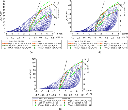
Relationship between pav and d in design models and in IBS Co1: (a) test 1; (b) test 2; (c) test 4
Relationship between pav and d in design models and in IBS Co1: (a) test 1; (b) test 2; (c) test 4
An estimation of KP was made for MC1 because one of the model inputs is KP, and it cannot be measured. KP inevitably changes due to the most probable increase in the RD during cyclic loading. The BSI model (BSI, 2011) fitted MC1 very well. The Vogt model (Vogt, 1983) yielded with softer output on small movements significantly less than d50. The best fit value of αp decreased from 0.016 to 0.008 during the loading cycles. This is comparable to the values proposed for αp in the literature. The factor C of the BSI model increased during the cycles from 15 to 23. The difference between MC1 and MC4 can be clearly observed from the results. Both models gave relatively good results for the MC4. The difference between the models was greatest for small movements. It seems that the soil underwent additional compacting and other permanent strains during the loading cycles, which led to the change in soil behaviour. The Finnish model (FTA, 2021), with du values of 2.5% and 3.5% of H produced results in the same range, but the simplified bilinear approach did not capture the small-strain behaviour.
The values of αp and C were affected by the RD. The relative movement d50/H in MC4 was 0.9%, 0.7% and 0.6% in tests 1, 2 and 4, respectively. Similarly, in MC1, d50/H = 1.3%, 1.0% and 0.75%, respectively. The change between MC1 and MC4 decreased with an increase in the RD. This is most probably due to the reduced, or negligible, increase in the RD during cyclic loading, with the higher initial RD in test 4.
The values of the design models fitted to tests 1–5 are shown in Table 3. From the results in Table 2, it can be concluded that KP is correlated with RD: KP = 14 when RD = 86% and KP reached a value of 26 when RD = 98%. The KP values were high, especially at the highest RD values, and this had an impact on the results. The values include uncertainties because the IBS might lead to high results due to the limited size of the soil containers.
Fitted model parameters from IBS test series
| Test | αp | KPa | C | ||||||||
|---|---|---|---|---|---|---|---|---|---|---|---|
| Co1 | Co2 | Co1 | Co2 | Co1 | Co2 | ||||||
| MC1 | MC4 | MC1 | MC4 | MC1 | MC1 | MC1 | MC4 | MC1 | MC4 | ||
| 1 | PCPP | 0.035 | 0.012 | 0.035 | 0.014 | 10 | 10 | 11 | 17 | 11 | 14 |
| 2 | PCPP | 0.018 | 0.009 | 0.017 | 0.010 | 15 | 15 | 15 | 23 | 17 | 21 |
| 3 | PCPP | 0.014 | 0.008 | 0.035 | 0.015 | 17 | 11 | 15 | 26 | 11 | 12 |
| 4 | PCPP | 0.014 | 0.008 | 0.012 | 0.008 | 22 | 25 | 15 | 26 | 19 | 26 |
| 5 | PCPP | — | 0.008 | — | 0.012 | 22 | 18 | — | 26 | — | 14 |
aEstimated value because the test could not measure this parameter
Furthermore, the final KP values were not reached because of the limitation of the maximum force of the IBS, and values for most dense soils are extrapolated (Mäntyranta, 2015). However, preliminary tests on fine sand and tests with lower RDs led to outputs where the failure surface was clearly within the soil container before the end wall of the IBS (Mäntyranta, 2011, 2015). On the other hand, the test soil material was very firm and had high strength, so the outputted KP values could be very high. The wall friction (r) in the tests was 2/3ϕ (Mäntyranta, 2015), which supports the high KP values.
4.3 Tests 3, 5, 8 and 10 with unequal RDs in IBS containers
The relationships between pav and d in tests 3, 5, 8 and 10 are shown in Figures 6, in which pav is plotted on the left-hand vertical axis and Kmob for Co1 and Co2 of the IBS are plotted on the right-hand vertical axes. Kmob was not equal for the same pav because the initial RD was different between the two containers (Co1 and Co2) of the IBS. The movements were strongly increased towards Co2 where the RD of the soil was lower (dCo2.max > dCo1.max), while pav was basically the same for both.
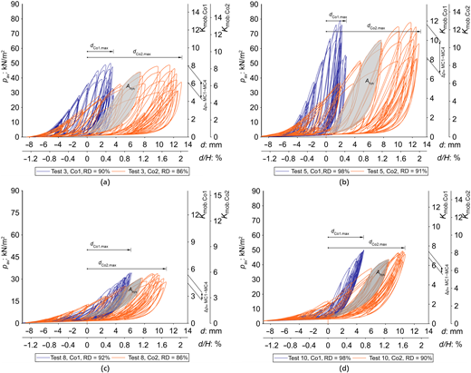
Relationship between pav and d in IBS Co1 and Co2: (a) test 3; (b) test 5; (c) test 8; (d) test 10
Relationship between pav and d in IBS Co1 and Co2: (a) test 3; (b) test 5; (c) test 8; (d) test 10
Tests 3 and 8 were conducted with almost equal soil RDs in the containers, as were tests 5 and 10. The difference was that the tests 8 and 10 included a CR layer while tests 3 and 5 had a PCPP layer. The CR reduced the unequal movements of the loading plates. The elastic springs decreased the uneven displacements of the loading plates in the most contracted state to avoid unrealistic movements. The increase in Kmob from MC1 to MC4 and the area of the hysteric loop (Ahys) was clearly reduced when the CR layer was used. In addition, the result for the highest RDs (test 10) showed rather linear behaviour during the cyclic loading. Based on the results, it seems that the CR layer reduced stresses, permanent strains and accumulating RD during cyclic loading.
In general terms, the soil behaved non-linearly while the CR behaved rather linearly. During the minor cycle, the soil exhibited more linear behaviour during reloading. Tests with nearly equal RDs without a CR layer (tests 1 and 5) and with a CR layer (tests 6 and 10) were conducted. Assuming the same kre values for tests 5–10 and tests 1–5, kCR could be estimated. This was done by assuming the stiffnesses in series resulting in:
A similar approach was adopted by Pietra et al. (2019) for non-linear soil behaviour with the Vogt model together with an elastic layer. The best fit to the results of tests 6–10 was reached with kCR = 27 MN/m3, which corresponds to a 1.3 MPa modulus of the CR for a 48 mm thick layer. This result is on the upper bound of predefined CR material properties based on research conducted by Tuominen (2008). This might occur for the case where the predefined modulus is a secant value, while the tangent modulus might yield higher values. Additionally, the larger grains of the crushed soil aggregate might partly push in the CR layer, leading to a higher apparent stiffnesses in IBS tests.
4.4 Comparison with monitoring results
The results obtained from monitoring of Haavistonjoki Bridge indicated the average earth pressure ( pav) as measured from the end screen at support T4. However, the distribution of the earth pressure cells (EPCs) was not uniform on the end screen of Haavistonjoki Bridge due to the limitation of a transition slab, which may result in slightly higher values of pav when the average of EPC results is used. Conversely, it was discovered that the wing walls had reduced the earth pressure at the corners due to friction between the wing wall and the embankment soil.
Furthermore, it was concluded that the earth pressures were higher directly under the transition slab because it tended to move less than the end screen (Laaksonen, 2004, 2011). For the sake of simplicity, only the mean values from the EPCs are compared. Also, the temperature of the embankment soil was used to indicate if the embankment soil was frozen or not. Haavistonjoki Bridge has undergone global longitudinal displacements. To compare the material behaviour, the displacement of the end screen was calculated based on the temperature variations and a constant value of the thermal expansion length of the superstructure. This was done in order to have comparable values without long-term longitudinal displacements occurring from settlement of the embankments and shrinkage of the superstructure.
Figure 7 shows a comparison of the results from Haavistonjoki Bridge and from test 1 in Co1 of the IBS. The unfrozen soil behaviour of the embankment of Haavistonjoki Bridge fits relatively well with the IBS result. The relative movement range (d/H) was wider in the IBS in comparison with the results of Haavistonjoki Bridge.
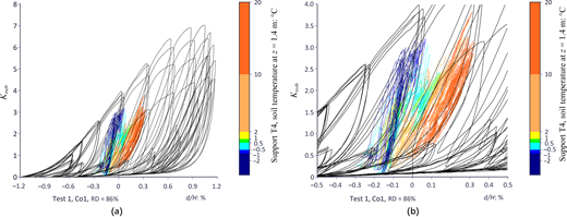
Comparison of results from (a) Haavistonjoki Bridge and (b) IBS test 1 (Co1)
Comparison of results from (a) Haavistonjoki Bridge and (b) IBS test 1 (Co1)
The RD of 86% is somewhat low when compared with the general requirement in Finnish guidance for RD = 90–95% (FTA, 2021). On the other hand, the magnitude of Kmob aligns with the design guidance (FTA, 2021). Furthermore, the real embankment was also subjected to multiple surcharge loads during the monitoring period. Settlement on the road embankment may have also occurred, making a direct comparison of results more uncertain. Much stiffer behaviour occurs when the embankment soil is frozen. Once the soil melted, the pressure decreased to the unfrozen level.
The movements of the loading plates in containers Co1 and Co2 in tests 3 and 8 and the movements of abutments T1 and T4 of Haavistonjoki Bridge between 10 October 2003 and 10 October 2010 are shown in Figure 8. The movement of the plates was found to be more uneven under higher earth pressure. The most uneven movements of the loading plates were measured during MC2, but the uneven movement stabilised during MC3 and MC4 in test 3. With negative movements, the springs between the plates and the frame of the test device reduced unrealistic eccentric displacement, imitating bridge structures that provide longitudinal stiffness. The CR layer clearly reduced the uneven movements. The uneven movements decreased during main cycles from MC1 to MC4.
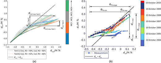
(a) Displacement of loading plates in containers Co1 and Co2 in test 3 and test 8 in the IBS. (b) Movements of abutments T1 and T4 of Haavistonjoki Bridge
(a) Displacement of loading plates in containers Co1 and Co2 in test 3 and test 8 in the IBS. (b) Movements of abutments T1 and T4 of Haavistonjoki Bridge
The results for Haavistonjoki Bridge for the first two years differed. The movements were highly concentrated to movements of the end support T4. The uneven movements decreased after the first two years. The difference was so large that the observed settlement of embankment T4 might partly explain the results. In addition, the bridge was finished in October 2004, and the first large movements of the end supports were due to contraction of the superstructure due to a decrease in temperature. It appears that the uneven behaviour of embankments may become more pronounced in this situation. In the case of expansion of the superstructure, abutment T4 showed approximately 20% higher displacements than abutment T1. This indicates a difference in the transversal stiffness of the embankment, which could be due to different RDs of the embankment soil between the end supports.
In the case of frozen soil, with high contraction of the superstructure, abutment T4 showed clearly higher displacements. It can be also seen that the movement caused by shrinkage of the superstructure accumulated more to negative movement of end support T4 than to end support T1. Therefore, the fact that embankment soil undergoes several loading cycles from a change in bridge length and from surcharge loading needs to be accounted for. This may result in a continuous change of the properties of the embankment soil.
During the monitoring period, it was observed that the road surface suffered settlements above end support T4, with the same support also having larger displacements from the temperature variations of the bridge superstructure (Laaksonen, 2011). A similar effect was observed from the IBS tests in the container where the movement of the loading plate was greater (Mäntyranta, 2015). This was concluded to be a consequence of the compaction and accumulation of permanent soil deformations resulting from repeated loading.
5. Conclusions
The development of earth pressure was much stiffer and the maximum values of the earth pressure were higher when the RD increased by only a reasonably small amount. In light of these findings, a potential explanation for the high variability of granular soil behaviour is the varying levels of RD compared with the assumptions made during structural design.
The findings of this work indicate that strain ratcheting has an influence on the outcomes, and the effect was more pronounced in soils with a smaller RD. This suggests that soils with lower RD may experience a greater accumulation of permanent strains.
The compared design models reproducing the transversal behaviour of the end screen were fitted with parameters for each main loading cycle in the IBS test. The parameter αp of model of Vogt (1983) model was in range 0.016–0.009 when a failure ratio (Rf) of 0.9 was applied in addition to the original model. The value of the factor C in the BSI model (BSI, 2011) was 10–15 during the first main cycles and 15–24 during the last main cycles. These values are lower than the value of 40 proposed in the design guidance (BSI, 2011). Earlier studies suggested that the value of 40 might be somewhat high (Kaufmann, 2008). In the context of the estimation of soil behaviour, the variation in KP across different RD levels had a substantial influence on the d–Kmob curve in the design models. Lower KP values are employed in design models, resulting in higher αp and C values.
The upper bound of cyclic loading will be reached with simplified design models and the results will be good, for example, for monotonically increasing movement caused by a temperature increase of the superstructure. In instances where the end screen undergoes unloading and subsequent reloading (i.e. minor cycles), the output is stiffer than expected based on design models. This behaviour is particularly evident in the case of braking load. The SSI at end screens is stiffer because the bridge end is pushed against the embankment and the other end is pushed out from the embankment. Even in the case of a simultaneous temperature increase of the superstructure, the other end behaves in stiffer manner during event of a brake load. And if the brake load takes place after a temperature decrease, both bridge ends might behave in a stiffer manner.
The different RDs in the embankment soil of an integral bridge might cause uneven movements of the bridge ends. The uneven movements can take place during loading cycles even with a reasonably small difference in the RD between bridge ends. However, the most uneven movements of bridge ends may occur during the most contracted situation with frozen soil conditions.
It seems possible that the stress levels and uneven movement of bridge ends can be reduced by using flexible material between the bridge end screen and the embankment soil. It is also conceivable that analysis of flexible layers could be carried out in a relatively simple manner.
Further research is necessary to study the creep effects of soil and the effects of the traffic surcharge loads. These might have an effect on the long-term behaviour of the embankment soil. The IBS may also be used to investigate and compare the effects of a wider variety of soil materials. Detailed numerical modelling with comprehensive soil material properties is needed to link material properties to the test outcomes between dense and loose granular soil behaviour, as noted by Bloodworth et al. (2012).
Acknowledgements
The authors thank the laboratory staff at Tampere University of Technology for their invaluable work during the research project and the Finnish Traffic Agency for funding this project.


