


Given that government financial assets represent a large proportion of gross debt accumulation, this study examines their impact on debt leveraging and potential returns on the gap between interest rates and economic growth (r-g).
This research focuses on the co-movements of r-g differentials, government financial assets and the primary deficit through a channel of gross debt, investment, external balance and ratings, using a sample of 27 European Union economies from 2000 to 2022. The following co-integration methods were estimated: (1) for the aggregate, panel quantile autoregressive distributed lags (QARDL), ARDL- pooled mean group (PMG) for panel data, implemented with a (PMG) and (2) ARDL-error correction (EC) for individual countries at a granular level.
While government financial assets drive short- and long-run debt trajectories, granular country heterogeneities reveal differentiated results for financial assets leveraging potential returns on the differential between interest rates and output growth (r-g). Government financial assets may enhance r-g, but may risk even undermining gains from primary deficit consolidation efforts. By comparing aggregate estimations with country granular approaches, outliers from non-statistically significant estimations reveal the epistemological limits of aggregation, statistics and probability theory, warning against overconfidence in such mere guidance tools, which are not safeguarding guarantees.
Statistical asymptotics and instability of non-independent and identical distributions may underestimate variance. Furthermore, skewness and leptokurtosis may benefit from extreme value theory. In addition, technological changes, policy regimes, geopolitical events and economic crises can change in-built long-run relationships.
Heterogeneity of government financial assets effects depend on socio and macrofinance conditions, advocating the principle of subsidiarity. Financial assets, such as sovereign wealth funds linked to natural resources, oil in Norway, copper in Chile, may benefit from financial assets assessments. The strengthening of democratic accountability calls for transparency about financial assets contribution to debt trajectories, r-g effects and risks of potential undermining primary deficit consolidations. Accounting reporting should appropriately disclose changes in assets value from exposition to market volatility, accumulation of holding costs due to constraints to asset liquidation, due to non-active secondary markets, or long investment horizons.
To strengthen democratic accountability, there should be transparency about their contribution to debt trajectories, r-g effects and risks to potential undermining primary deficit consolidation. Their performance depends on financial markets and socio- and macro-finance conditions, calling for the principle of subsidiarity.
Rather than the traditional emphasis on government debt, this study examines the leverage effect on the gap between interest rates and economic growth (r-g differential). While the literature primarily addresses stock-flow adjustments (SFAs), the focus is narrowed to financial assets underlying government interventions on the supply side of the economy. Evidence is provided on the risks of financial assets undermining primary deficit consolidation efforts. While the literature highlights the short and medium terms, estimates are divided into short-term dynamics and hypothetical in-built long-run cointegrations. Panel aggregation is compared with granular estimates, uncovering heterogeneities and supporting governance subsidiarity. Support for statistical pluralism is provided by comparing results and methodological limitations.
1. Introduction
Government borrowing capacity is considered an important factor in a country’s development potential. However, debt is not an end in itself; rather, it is a mean of generating greater potential growth (otherwise unattainable) beyond borrowing costs—the differential between the interest rate and GDP growth (r-g).
While government debt and deficit binomial are at the heart of public finance, government financial assets are typically excluded from fiscal spending accounts, circumventing deficit limits and underlying large and persistent discrepancies between changes in public debt and primary deficits. This ambiguity raises the research question: What is the leverage effect of financial assets, in interaction with the primary deficit, on expanding or contracting government financing capacity to generate growth exceeding borrowing costs?
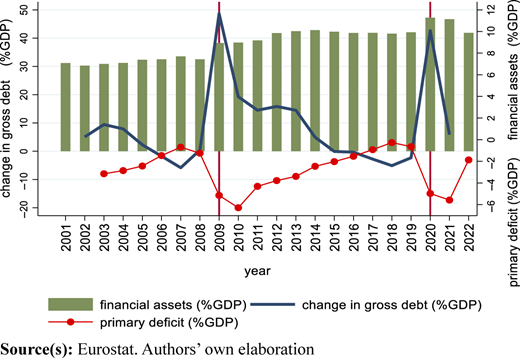
In the European Union, increases in government financial assets coincide with two spikes of primary deficits and gross debt around 2009–2010 and 2020–2021 (Great Financial Crisis and the COVID-19 pandemic). These episodes were followed by consolidations, with larger reductions in primary deficits than in financial assets (Figure 1).
The innovative contributions of this study to the literature are as follows: first, although traditional sustainability assessments focus on debt consolidation, this work posits that government debt is not an end in itself; rather, it is a means of leveraging the expansion of the financing capacity to generate growth (which otherwise would be unattainable), beyond borrowing costs (r-g differential). Second, while the literature is centered mainly on stock-flow adjustments (SFAs), this study narrows the scope to financial assets, which underlie government interventions on the supply side of the economy. Third, evidence is provided on the risks of financial assets undermining primary deficit consolidation efforts. Fourth, while the literature on SFAs usually highlights short and medium terms, financial asset estimates were divided into short-term dynamics and hypothetical in-built long-run cointegration. Fifth, panel aggregation is compared with granular estimates, uncovering significant heterogeneities depending on country specificities and strengthening the support of subsidiarity principles. Sixth, the hypothesis that financial assets and the primary deficit were strategically managed together was rejected only in three countries. Seventh, this study supports statistical pluralism for policy decision-making by comparing results and methodological limitations.
The rest of the paper is organized as follows: Section 2 reviews the relevant literature. Section 3 discusses the methodological approaches, data and sources. Section 4 reports the results of aggregate panel analysis and individual countries' estimates. Section 5 discusses the results, policy implications, limitations and future research. Section 6 summarizes the main conclusions. Furthermore, in the Appendix, the intertemporal budget constraint (IBC) is derived. The Supplementary file displays all estimation coefficients and respective technical details.
2. Literature review
The theoretical framework for the IBC is grounded in traditional public finance debt sustainability, advocating that present value obligations should not exceed primary balances (Debrun et al., 2020).
Government indebtedness was justified by Barro (1979) in the “tax smoothing hypothesis,” limiting changes in distortionary taxes, keeping an optimal tax rate across time. Only permanent expenditures would be relevant for taxation, whereas temporary changes would leave taxes unaltered, with borrowing used to cover government financing needs [1], such as during wartime and economic depressions, which are viewed as transitory phenomena. However, it can be argued that the time frame may be long and characterized by persistent dynamics, justifying a co-integration approach.
Although, according to Romer and Romer (2019), countries with lower debt-to-GDP would benefit from higher debt levels to support economic crisis, attention has been drawn to the risks of large debt surges leading to persistent lower economic growth, especially when the initial debt level was already high, as noted by Jalles and Medas (2022). In this context, significant attention has been given to government debt, which is driven not only by primary balances, but also by stock-flow adjustments (SFAs) [2]. They were found to be as important as primary deficits in explaining debt surges and consolidations (Abbas et al., 2011). Weber (2012) documented SFAs inducing significant debt increases in 14 European Union countries, playing a minor role in explaining debt decreases. Afonso and Jalles (2020) reported SFAs’ contributions to significant debt-to-GDP increases. Jaramillo et al. (2017a) found that peaks in SFA accumulation were associated with public debt and financial market distress, leading to a higher probability of non-declining debt paths.
On the policy side, von Hagen and Wolff (2006) showed how governments strategically use SFAs to circumvent fiscal rules, under-reporting deficits in the European Economic and Monetary Union. Correlations between budget transparency and SFAs denote the low quality of budgetary institutions, creating space for fiscal gimmickry (Alt et al., 2014), emphasizing the need for fiscal transparency and reducing off-budget operations. Jaramillo et al. (2017a) hypothesized that SFAs are not only residual values; rather, they can intentionally be used as creative accounting to circumvent fiscal rules, undermining two core features of prudent fiscal policy: transparency and sustainability (Milesi-Ferretti and Moriyama 2006). Alt et al. (2014) and Reischmann (2016) showed that SFAs were tactically used in pre-election periods to attract voters. In contrast, for Afonso and Jalles (2020), SFAs neither correlated with fiscal rules transparency nor with budget deficit manipulation. SFAs were found to have methodological effects on overly optimistic fiscal forecasts, advocating for their inclusion in debt sustainability accounting (Acosta-Ormaechea, 2020), akin to measuring public debt costs as proposed by Hall and Sargent (2011) and Ellison and Scott (2020).
This literature narrowed the scope to financial assets, which are components of SFAs and underly government interventions in the supply side of the economy. For example, for Abbas et al. (2020) nationalizations, subsidies and loans to the economy accounted for, on average, about 90% of SFAs during the Great Depression.
The focus on financial assets expands the literature to include their impact on r-g differentials, beyond their impact on debt, extensively analysed in Seiferling (2013) and their long-term contribution to debt in Eichengreen et al. (2019). For Afonso and Alves (2019), higher interest rates penalize debt service, requiring non-attainable growth, leading governments into liquidity shortages and austerity (Afonso et al., 2021).
This study integrates a transmission channel of effects on financial assets from scattered literature, such as interest rate channels, which reflect financial markets liquidity and credit risks (Jaramillo et al., 2017b). It also integrates the impact of financial assets through external trade accounts. In the twin deficit hypothesis by Afonso and Coelho (2023), cyclically adjusted primary budgets determined current accounts. For Perla et al. (2021), economic growth benefits from trade, increasing export opportunities, since foreign competition induces faster technological adoption. This literature dates back to Solow (1956), who studied the positive impacts of foreign direct investment on economic growth by introducing new technology into production. This was subsequently augmented by Mankiw et al. (1992) accounting for the accumulation of human and physical capital, which may explain heterogeneities among countries.
This study examines the heterogeneous effects of government financial assets following the line of inquiry established by Bhandari et al. (2017), who focused on heterogeneous multi-agents with uncertainty and incomplete markets, which modelled planners’ preferences for minimizing the welfare costs of transfer fluctuations, relying on asset returns, making policies over the business cycle differ from those in Ramsey’s representative agent outcomes.
3. Methodology
3.1 Research design
The research was designed, as illustrated in Figure 2, to answer the following question: What are the impacts of financial assets, when interacting with the primary deficit, on the government’s financing capacity, particularly in leveraging potential returns on growth relative to borrowing cost differentials? Effects on r-g differentials depend on whether debt burdens grow or shrink, and whether the respective interest rates on debt (r) exceed or fall below economic growth (g). This study focuses on the r-g effects mediated by investment, external trade balances and ratings.
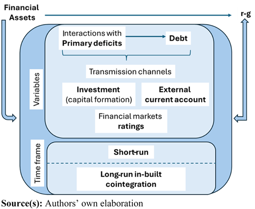
These effects are inherently long-run phenomena, while short-term analysis may miss persistent long-term co-movements. Short-term dynamics and long-run co-integration were estimated: (1) for the aggregate, panel quantile autoregressive distributed lags (QARDL) and ARDL for panel data with a pooled mean group (PMG); and (2) heterogeneity of results implied estimating granular ARDLs for individual countries.
3.2 Data and variables
The sample of financial assets for 27 European Union countries [3] ranged from 2000 to 2022. Quarterly data from Eurostat were used, expressed as a percentage of GDP and annualized. Besides financial assets (FA), primary deficit (PD), gross debt (GD) and net debt (ND), the study focused on the channels of gross capital formation (GCF) and external trade balances (CAB). Sovereign bond ratings were retrieved from the World Government Bonds [4] site.
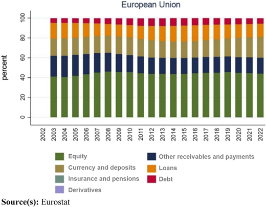
Net change of financial assets (purchases minus sales), depreciations/appreciations—mostly of equity and investment fund shares—currency and deposits, as well as loans and debt were included (Figure 3).
3.3 Analytical approach
The theoretical approach is translated into a government IBC, fully derived in Appendix and summarized in Section 3.3.1. The government borrowing constraint was formalized by an intertemporally balanced budget framework in present value terms, following Hamilton and Flavin (1986). Debt sustainability, satisfying the IBC, was derived from the difference between safe interest rates and economic growth and is closely related to Bohn’s (1995, 1998) work. Besides the primary deficit, the IBC equation also accounts for government financial assets, since they explain large and persistent discrepancies between changes in public debt and budget deficits, as outlined in the stock-flow adjustment approach by Weber (2012).
The theoretical relationships of the IBC were specified with econometrically testable equations and identification conditions, to meet the estimation requirements of econometric methods. Persistent paths of the IBC were approached with a long-run in-built stationary equilibrium and dynamic short-run corrections following the general framework of Castle et al. (2021). Specific techniques are detailed in Section 3.3.2.
3.3.1 Government intertemporal budget constraint (IBC)
The following summary of the government IBC is fully derived in Appendix.
Past debt stock is carried forward, compared with the present value of future income, including a terminal debt stock. At the end of any previous period t−1, debt progression on the outstanding legacy of nominal debt stock changes in the present period t by: debt service, ; debt change (amortizations and issues) ; nominal primary budget balance and change in government financial assets .
Taking real government debt and real output growth as a function of real GDP , adjusted for inflation (GDP deflator), the leverage effect at any period t, represented by the differential between real interest and real growth rates ( differential), will depend on outstanding debt stock legacy ; change in debt stock ; primary balance and change in government financial assets .
The expected value of the current outstanding debt at period t, , evolves according to the expected net present value of future primary budget balances , changes in government financial assets , accounting for terminal values (assuming a null transversality condition):
3.3.2 Econometric specification
This study focused on the leverage effects of government financial assets (ΔFA), interacting with the primary deficit (PBB), in amplifying or shrinking r-g, through the transmission channel: financial market conditions proxied by changes in sovereign bond ratings (Δratings), gross capital formation (GCF) and external trade balances (CAB).
The study began at an aggregate level, applying quantile panel ARDL and panel PMG cointegration. Since samples were organized in 27 countries, data panel dimensions may statistically be interpreted as replicating 27 blocks, resulting in a number of N cross-sections larger than the size of the fixed time periods (N > T). Because of the cross-sectional dimension of data, data dynamics were not restricted to the panel specifications, since fixed-T, large-N asymptotics were estimated (in-depth technical details in Wooldridge, 2010).
Heterogeneity of results demanded a more granular approach, proceeding towards individual country ARDL specifications. Estimations of error correction terms and short-run VARs provided adjustment coefficients and in-built long-run co-integration equations. Since inferences are asymptotically invalid on mis-specified models with heteroskedasticity and serial correlation, diagnostic tests were estimated and standard errors were corrected, as detailed in the Supplementary file.
3.3.2.1 Quantile panel QARDL
Estimates of quantile-dependent r-g differentials employed a panel quantile autoregressive distributed lag (QARDL), as an extension of the autoregressive distributed lag, adapted from Cho et al. (2015):
where α1 represents short-run coefficients and βi/β0 (i≠0) represents long-run coefficients (Table 1). False results from heteroskedasticity, skewness, multicollinearity (Dawar et al., 2021) and structural breaks (Selmi et al., 2018) are avoided. As a caveat, this is only applied to first differences and not beyond (Arshed et al., 2022).
Quantile panel ARDL
| Q1 | Q2 | Q3 | Q4 | ||
|---|---|---|---|---|---|
| Short-run coefficients | Δratings | −0.535*** | −0.429*** | −0.903*** | −1.637*** |
| CAB | −0.399*** | −0.289*** | −0.405*** | −1.069*** | |
| GCF | −0.704*** | −0.608*** | −0.725*** | −1.096*** | |
| ΔFA | −0.003*** | 0.034*** | 0.057*** | 0.349*** | |
| Convergence | r − g | −0.154*** | −0.130*** | −0.145*** | −0.283*** |
| Lag coefficients | Δratings | −1.300*** | −0.899*** | −1.830*** | −5.286*** |
| CAB | 0.024*** | 0.001*** | −0.042*** | 0.073*** | |
| GCF | −0.043*** | 0.011*** | 0.041*** | −0.025*** | |
| ΔFA | −0.087*** | −0.047*** | −0.042*** | −0.471*** | |
| Long-run coefficients (1) | Δratings | 8.442*** | 6.915*** | 12.621*** | 18.678*** |
| CAB | −0.156*** | −0.008*** | 0.290*** | −0.258*** | |
| GCF | 0.279*** | −0.085*** | −0.283*** | 0.088*** | |
| ΔFA | 0.565*** | 0.362*** | 0.290*** | 1.664*** |
Note(s): *, ** and *** significance at 10%, 5%, 1%
(1) Long-run coefficients are the ratio of lag coefficients to convergence coefficients
Source(s): Authors’ estimations
3.3.2.2 Panel PMG cointegration
To choose a re-parametrized ARDL specification for panel data, the Hausman specification test was applied, estimating whether individual effects were correlated with or independent of the explanatory variables. Pooled mean-group (PMG) was compared with dynamic fixed effects (DFE), with equality assumed across panels (results in Section 4.1.2). Since the test did not support DFE specifications, PMG was estimated (Pesaran et al., 1999), with long-run effects equally constrained across panels, but differentiating equilibrium correction terms and short-run coefficients for each country i in period t, as follows:
Xit is the vector of co-integrating variables: (1) changes in ΔFA-financial assets; primary deficit- PBB; (2) channels of GCF investment (gross capital formation); CAB external trade balances and ratings. Parameters are θi speed of adjustment; β’s long-run coefficients; the error correction terms; and the short-run dynamics coefficients.
Effects on r-g through debt, applying panel PMG, were parallel to previous specification (3), but matrix Xit of explanatory variables is now the vector of changes in government bond ratings, changes in gross debt (Δgross debt), and net debt (Δnet debt) (Table 4 of the Supplementary file).
3.3.2.3 Individual country ARDLs
Individual countries’ ARDLs were estimated for three specifications: (1) a twin model (TM) with financial assets, primary deficit and gross debt together; (2) financial assets as a standalone model (SM) with gross debt and (3) primary deficit as a SM with gross debt. Comparing coefficients estimates of standalone (SM) and twin (TM) specifications allowed the estimation of whether financial assets and the primary deficit were interrelated, or, instead, independently affecting gross debt.
To disentangle how much the data contained information about short-run and hypothetical persistent long-run co-variabilities, in feedback corrective loops towards an in-built long-run equilibrium, country-specific autoregressive distributed lags, reparametrized in the so-called error-correction form, ARDL (p, q)-EC, were estimated with lag orders p and q for each country i and period t:
is the matrix of cointegrating variables: changes in financial asset holdings ΔFA and primary deficit PBB.
Reparametrizing the above Equation (4), taking the speed-of-adjustment coefficient and long-run coefficients , into account, the error correction (EC) for country i includes a p−1 lag vector error correction (VEC), that is, the underlying vector autoregression VAR order minus 1, as pointed out in Lütkepohl and Krätzig (2004):
Further technical details are found in the respective tables of the Supplementary file.
Impulse responses (IRFs) and variance decompositions (VD) were based on structured VAR information sets, with the target variable being the change in gross debt and exogenous shocks including changes in financial assets and the primary deficit. Forecast-error decompositions were based on Cholesky’s approach, known as orthogonalized IRFs. Only the larger estimates are reported (Section 4.2).
4. Results
4.1 Aggregate panels
4.1.1 Quantile panel ARDL
In the short-run (Table 1), in all quantiles of the r-g distribution, the lowest coefficients were estimated for financial assets, negative (−0.003) in the first quantile and positive afterwards (adverse r-g effects). The coefficients for ratings, investment and external trade balance coefficients were negative across the entire r-g distribution, contributing to a favourable leverage. At the lowest 50% quantile, the largest coefficients were driven mostly by investment (−0.704; −0.608), followed by ratings (−0.535; −0.429). At the upper 50% quantile of larger r-g differentials, ratings had the most significant impact (−0.903; −1.637).
In the long-run, the convergence speed coefficient towards equilibrium was negative and statistically significant, however, denoting a rather low adjustment (−0.130 to −0.283). Rating coefficients were preponderant, followed by financial assets. The impacts of investment and external trade balances were lower.
In the short-run, the effect of financial assets on r-g differentials was lowest (−0.003 to 0.349) with a positive sign at the upper 75% quantile, denoting an unfavourable leverage (increasing r-g). In contrast, the long-run effects of financial assets on r-g were the second largest (after ratings) and positive, also denoting an unfavourable leverage, increasing r-g (lower economic growth compared to higher debt burden). Coefficients were higher at the tails of the quantiles (0.565; 1.664) and lower in the middle quantiles (0.362; 0.290), which is characteristic of leptokurtic distributions. Long-run estimates highlight the leading role of ratings, with increases towards r-g, reducing the space for output growth below the interest burden.
Capital formation was second in magnitude in the short-run, influencing the decline of r-g, more significantly than external trade, with a favourable leverage effect that expands the space for output growth above interest rates. However, in the long-run, at the tails of the distribution, it contributed to positive (r-g deteriorating) effects (0.279; 0.088).
External trade coefficients were third in magnitude (−0.399 to −1.069), mostly negative in the middle quantiles (r-g improvement). On the contrary, above quantile 50% and below quantile 75%, the effect was positive (unfavourable impact increasing r-g). These estimates are consistent with external trade balance coefficients being lower in the short-run and higher in the long-run, since trade opportunities take time to materialize.
4.1.2 PMG – financial assets and primary deficit interactions
The choice of panel PMG cointegration was preceded by Hausman specification tests, which, except in one model, as explained below, did not accept fixed effects specifications (Table 2). Two models were tested: (1) financial assets and primary deficit effects on r-g, through investment and external trade channels and (2) financial assets and primary deficit effects on r-g.
Panel ARDL Hausman (1978) test
| Channel: investment, external trade | Channel: gross and net debt; ratings (3) | |
|---|---|---|
| Ratings (1) | (a) (2) | |
| H0: difference in coefficients not systematic | ||
| = −116.67 (b) (e) (f) | Prob > = 0.120 (b) | = −46.27 (b) (f) |
| Prob > = 0.997 (c) (e) | = −548.22 (c) (f) | |
| Prob > = 0.0000 (c) (d) (e) | ||
Note(s): (a) Countries without ratings or stable ratings: Denmark, Estonia, Germany, Luxembourg, Netherlands
(b) Estimates the contrast variance for tests of exogeneity and overidentification. Covariance matrices are based on the estimated disturbance variance from the efficient estimator
(c) Estimates use all equations, basing (co)variance matrices on disturbances variance estimates from efficient estimators
(d) Includes constants, the estimated intercept(s), in model comparison
(e) The difference between the variance-covariance matrices of the models is not positive definite
(f) The model fails to meet the asymptotic assumptions. However, the seemingly unrelated estimation (SUEST) is unable to generate required scores for the DFE model
Source(s): Authors’ estimations
For the specification with ratings (column 1), the chi-square was negative, failing to meet the Hausman test’s asymptotic assumptions. However, seemingly unrelated estimation (SUEST) could not be applied because DFE did not generate scores. Using all equations, the p-value was 0.997, but since the difference in variance matrices was not positive definite, it was not accepted that the PMG was a more efficient estimator. For the specification without ratings (column 2), the p-value was just above 10%; thus, the PMG estimator was not rejected.
The model of financial assets and primary deficit effects on r-g, by gross and net debt through the ratings channel (column 3), was the only model with a p-value <0.05, but the difference of variance matrices was not asymptotically positive definite. Considering heterogeneities across panels, a PMG was also implemented, allowing for country-differentiated short-run and equilibrium correction terms.
4.1.2.1 Channel – investment, external trade and ratings
In the long-run, negative and statistically significant error correction terms (Table 3 of the Supplementary file) implied that the processes were converging to an in-built equilibrium. Co-integration coefficients were negative for all variables, pointing to favourable r-g leverages, increasing growth above interest rates. Primary deficit contributions to r-g (−0.671 in the full model with ratings; −0.684 without ratings) were larger than those from changes in financial assets (−0.153; −0.154). Ratings were the second largest contribution (−0.637), followed by investment (−0.629; −0.521) and external trade balance (−0.385; −0.243).
Short-term coefficients of financial asset contributions to r-g were significantly larger than those of the primary deficit in most countries, except in Luxembourg and the Netherlands. Comparing statistically significant coefficients, the effects predominantly originated from financial assets towards increasing r-g (from a minimum of 10.191 in Greece to a maximum of 66.996 in France). In contrast, coefficient estimates were lower regarding the primary deficit’s effects on the r-g differential declines (−0.485 in Cyprus, −3.530 in Croatia). France’s estimates of financial asset coefficients displayed the largest deterioration (increase) of r-g, with debt service costs rising steeply above those of comparatively lower counterparts from growth, followed by changes in financial asset coefficients for Italy (58.915) and Belgium (56.458). The lowest financial asset coefficients were observed in Greece (10.191), with the primary deficit not statistically significant.
For those countries with statistically significant investment and external trade balances, most estimates reported negative coefficients, favourably impacting r-g declines, except for the positive coefficients of external account balances in Latvia (1.384) and Romania (2.813).
Countries where investment had a larger effect on r-g were Italy (−5.459), Spain (−4.426), France (−3.877), Denmark (−3.310), Sweden (−2.961), Lithuania (−2.705) and Austria (−2.583), denoting predominant economic growth over interest rates. Countries where external trade balances had a greater impact on r-g, reinforcing growth over debt service, were estimated for Italy (−3.268), France (−2.853), Denmark (−2.394) and Germany (−2.108).
4.1.2.2 Channel – gross and net debt
Only panel aggregate gross debt estimates were statistically significant (Table 4 of the Supplementary file). All equilibrium correction terms were positive, implying that long-run processes were not converging to an in-built long-run equilibrium. Instead, they were explosively widening the gap between interest burden and output growth, questioning long-run co-integration from either gross or net debt, and validating the use of gross debt (accounting for changes in financial asset holdings), rather than net debt, as significant indicators of potential leveraging effects (r-g).
In the short-term, ratings reported higher coefficients impacting r-g, well above those of gross and net debt. For many countries, the effect of ratings was negative, towards decreasing (improving) r-g differentials (Belgium, Ireland, Italy, Latvia, Lithuania, Malta, Poland, Portugal, Romania, Slovakia, Slovenia, Spain and Sweden). Exceptions were Denmark, Germany and the Netherlands (due to rating stability), and Austria, France, Cyprus and Greece with increasing effects on r-g. These estimates highlight the predominance of financial markets in determining r-g differentials.
In all countries, gross debt coefficients (accounting for financial assets) were larger than those of net debt, with the highest values in Romania (0.908), Latvia (0.609), Croatia (0.552), Malta (0.531) and Lithuania (0.527). Net debt (without financial assets) showed statistically significant negative coefficients, denoting an impact on decreasing r-g differentials (interest rates below economic growth).
4.2 ARDLs for individual countries
Aimed at building an aggregation rationale for country ARDLs, the results (Figure 4 and Table 5 of the Supplementary file) were organized into clusters according to statistical commonalities and the coefficients of financial assets and primary deficit.
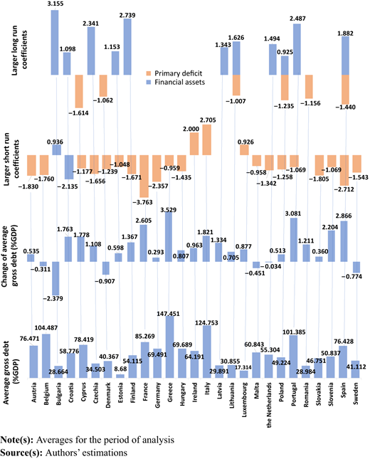
In a small group of four outlier countries (cluster C3.2), estimates of financial assets were statistically significant only in the short-run, rejecting the hypothesis of comoving together with gross debt in the long-run, and downplaying the effectiveness of policies managing government debt with financial assets.
4.2.1 Cluster C1 ‒ largest coefficients from financial assets in the short- and long-run
The predominance of financial asset contribution to gross debt was statistically significant only in Bulgaria and Latvia. Bulgaria’s adjustment term in the TM was one of the highest in the sample, with deviations from the in-built long-term equilibrium corrected at 75% adjustment speed. Long-run effects of financial asset contributions to building up gross debt were larger than those of primary deficit containment. On average, the decline in gross debt was larger (−2.379% of GDP), whereas the gross debt level remained low (28.644% of GDP). Latvia’s largest coefficient was also driven by financial assets (in the long-run 1.343 as a SM and 0.944 in the TM), justifying an average gross debt increase of 1.334.
4.2.2 Cluster C2 ‒ alternance of predominance of assets and primary deficit
Belgium’s estimates were the largest long-term contributions of the sample of financial assets to gross debt (3.155 in the SM). In the short-run, primary deficit coefficients were larger than those of financial assets (larger at lags, −1.047 in the SM). On average, gross debt was reduced by 0.311% of GDP.
Ireland’s long-run coefficients were larger for financial assets. However, the adjustment term (−3.582) was highly oscillatory. In the short-run, primary deficit predominated, with the largest coefficient (2.000 in the SM) contributing, on average, to 0.963% of GDP gross debt increase, accounting for 64% of GDP.
In Germany, in the long-run, financial assets assumed preponderance (but with the bounds test not statistically significant and a low adjustment term of −0.178), contributing to an average gross debt of 69% of GDP and a 0.292% increase in GDP. The preponderance of financial assets is illustrated by larger IRFs (Figure 5), estimating that a shock of one standard deviation in financial assets influences gross debt growth up to approximately 3.383% (at lag 12), whereas VD explained more than 30% of gross debt variance. In contrast, primary deficit estimates were lower, with the IRF at 1.86% and the VD up to 29.8%, both at lag 12.
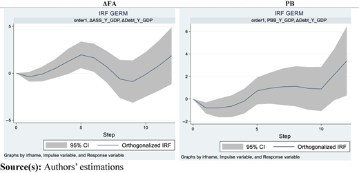
Impulse responses (IRFs) of gross debt from financial assets and primary balance (Germany)
Impulse responses (IRFs) of gross debt from financial assets and primary balance (Germany)
In Austria, while the largest short-run coefficients for the primary deficit reduced gross debt growth, in the long-run, the predominance of financial assets contributed to gross debt growth (0.928 as the SM, although the bounds test is not statistically significant). Long-run debt containment from primary deficit consolidation was low, resulting in a slight amplification of average gross debt (0.535% of GDP).
In the TM, the larger coefficient for Cyprus’ long-term financial assets (2.341 in the SM) was reduced (0.656 for financial assets; −1.631 for the primary deficit). The adjustment speed corrected deviations from the in-built equilibrium at 50% for each period. In the short-run, primary deficit coefficients were larger (−1.296 at lag 7) than those of financial assets. Primary deficit consolidation was undermined by financial assets amplifying gross debt growth, resulting in a 1.778% increase in gross debt relative to GDP and an average of 78% of GDP.
In the short-run, on average, the Netherlands’ gross debt of 55% of GDP decreased by 0.034% of GDP, mostly driven by the primary deficit rather than by financial assets. Effects alternated between increasing and decreasing gross debt. In the long-run, the adjustment coefficient was at most −24%, with larger coefficients from financial assets driving gross debt growth, which increased slightly on average (0.034% of GDP).
Spain’s long-term financial asset coefficients (1.882 in the SM) reported a slow adjustment term of −10.8%. Coefficients declined in the TM, conceding predominance to the primary deficit (−1.141) and reducing gross debt growth. Lower coefficients of the TM weaken the hypothesis that financial assets and the primary deficit were strategically managed together. With an impulse of a one standard deviation shock from financial assets impacting gross debt growth by approximately 2%, the effects alternated (Figure 6): decreasing gross debt growth from lag 1 to 4 and increasing it from lag 8 to 10. IRFs from the primary deficit were lower, while VD of financial assets explained up to 37% (at lag 11) of gross debt growth variance, which was also larger than those of the primary deficit (only 7%).
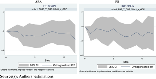
Impulse responses (IRFs) of gross debt from financial assets and primary balance (Spain)
Impulse responses (IRFs) of gross debt from financial assets and primary balance (Spain)
Hungary’s primary deficit was statistically significant and preponderant in the SM, but only in the short-term (−1.435 at levels and 1.137 at lag 1). In the long-run, the effects on financial assets (0.649) predominated, amplifying gross debt growth more than primary deficit containment (−0.485). The speed of equilibrium corrections was one of the highest in the sample: deviations from the in-built equilibrium were corrected at 78.6% for each period. On average, gross debt increased by 0.807% of GDP, reaching 69.689%.
Lithuania’s low gross debt (on average 30.855% of GDP) slightly increased by approximately 0.705% of GDP, mainly driven by financial assets, which reported the largest long-term coefficient, while primary debt contributed less to the containment of gross debt growth.
Estonia’s average gross debt was the lowest in the sample, below 9% of GDP. In the short-run, the effects of primary deficits were larger than those of financial assets. In the long-term, primary debt coefficients were not statistically significant, while financial assets contributed to gross debt growth (0.598% of GDP).
4.2.3 Cluster C3 ‒ predominance of primary deficit
The largest group of countries reported estimates with higher coefficients of gross debt, predominantly resulting from the primary deficit.
4.2.4 C3.1 ‒ financial assets statistically significant in the short- and long-run
Although the effects on gross debt originated predominantly from primary deficit, financial assets were also statistically significant in the short and long-run.
Denmark’s adjustment term, in the TM (financial assets and the primary deficit), was one of the largest in the sample, estimating a correction speed of deviations from the in-built long-run equilibrium of 75% for each period. In the long-run, the primary deficit was predominant, reducing gross debt growth (−0.907) to a stock of only 40% during the period.
Luxembourg reported one of the lowest gross debts (on average 17% of GDP), with a slight increase over the period (on average 0.877% of GDP). Larger coefficients were estimated for the primary deficit, both in the short and long-run, reducing gross debt growth. This became one of the largest adjustment coefficients in the sample, correcting approximately 78% of the deviations from the in-built equilibrium each period.
Portugal’s short- and long-term dominance stemmed from the primary deficit declining and a slowdown in gross debt growth; however, the adjustment coefficient was relatively moderate (−28.7%). In the short-term, at level values, the effect of financial assets was 0.678 and that of primary deficit was −0.615. These combined effects concurred to a 3.08% of GDP average gross debt growth increase—the second largest in the sample—reaching an average gross debt of 101% of GDP.
Poland’s primary deficit dominated gross debt containment. The adjustment coefficient of the TM was lower (−6.6%) compared to the SMs (20.4%; 69.3%), challenging the hypothesis of strategically managing financial assets and the primary deficit together. Gross debt was, on average, approximately 49% of GDP during the period, increasing by an average of 0.513% of GDP.
Sweden’s dominant primary deficit and gross debt containment converged at a −49.7% speed of adjustment towards the SM equilibrium, which was larger than the −29.4% of the TM. This also weakens the hypothesis that financial assets and the primary deficit are strategically managed together. On average, gross debt growth declined by 0.774% of GDP, reaching 41%.
Greece’s average gross debt was the sample’s highest (147% of GDP), a GDP increase of approximately 1.778%, with financial assets being the only source of statistically significant long-term coefficients.
Slovenia’s increase in gross debt was, on average, 2.204% of GDP, reaching 50.8%. Although the long-term effects were predominantly driven by the primary deficit reducing gross debt growth, they were adjusted at a speed below 30%. Short-term effects of both financial assets and the primary deficit increased gross debt.
Slovakia’s average gross debt, at 47% of GDP, reported a slight increase of 0.3% of GDP. This does not reflect the predominant effect of the primary deficit in reducing gross debt; instead, it highlights the influence of financial assets in driving gross debt growth.
Other countries also reported statistically significant effects on financial assets, which were lower than primary deficit coefficients in both the short- and long-run. Czechia’s average gross debt of 34% of GDP increased, on average, by 1.108% of GDP. Romania’s low gross debt, on average 29% of GDP with an increase of 1.211% of GDP, reflected the predominance of primary deficit restraints. Malta’s primary deficit containment reflected an average decrease in gross debt of −0.451% of GDP and an average gross debt level of 61% of GDP.
4.2.5 C3.2 ‒ Financial assets statistically significant in the short-run and not statistically significant in the long-run
Changes in financial assets were not statistically significant in the long-run, and their influence on gross debt was only in the short-run.
Croatia’s long-run primary deficit effects on gross debt converged to the in-built equilibrium at a rather slow adjustment. Short-term effects were larger, mostly driven by the primary deficit, increasing gross debt, on average, by 1.763% of GDP, reaching 58.776%.
In the long-run, France’s gross debt containment, driven by the primary deficit, was the only statistically significant coefficient, with a 47.9% speed of adjustment. In the short-run, the primary deficit was preponderant than the financial asset coefficients, with opposite effects on gross debt. Gross debt growth predominated, averaging 2.605% of GDP and reaching 85%.
Finland’s primary deficit effects surpassed financial assets in the short and long-run. Co-integration of primary deficit, financial assets and gross debt was not statistically significant, nor was short-run coefficients of financial assets in the TM. The predominant primary deficit coefficients in the SM decreased gross debt growth, with a larger effect in the short-run (−1.671) than in the long-run (−0.456), at a 41% adjustment speed. Gross debt increased, on average, by 1.367% of GDP, reaching only 54%.
Italy’s gross debt was the second largest in the sample (on average 124.7% of GDP). Long-run equilibrium was not statistically significant. Standalone coefficients were larger than those in the TM, suggesting a less significant strategic management of financial assets and the primary deficit together. In the SM, short-run effects of primary deficits contained gross debt growth (−2.520 at lags), while amplifying at lag 1 (2.705), which might explain Italian gross debt as the second largest in the sample (an average of 124.7% of GDP and an increase of 1.821% of GDP). In the TM, the effects of the predominance of financial assets are illustrated by an increase in gross debt growth of up to 1.355% (at lag 7), exceeding the highest coefficient of the primary deficit (−0.938% at lag 3). The alternance of effects is illustrated (Figure 7) by IRS and VD of financial assets, which explain more than 40% of gross debt growth variance—larger than that of the primary deficit (7% at most, above lag 11).
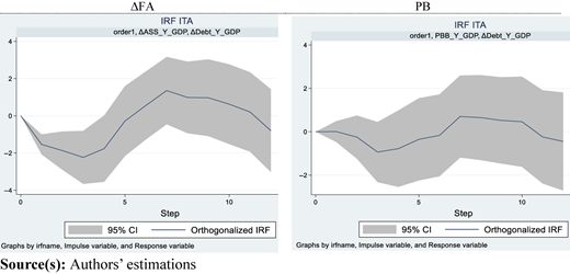
Impulse responses (IRFs) from financial assets and primary balance to gross debt (Italy)
Impulse responses (IRFs) from financial assets and primary balance to gross debt (Italy)
5. Discussion
Statistically significant estimations revealed heterogeneous impacts of financial asset interactions with the primary deficit, either expanding or contracting government debt financing and either generating higher or lower growth beyond borrowing costs.
5.1 Theoretical implications
In the long-run, estimates warn about the risks of financial assets contributing more to gross debt accumulation than to primary deficit consolidation efforts. These opposing effects have an impact on debt sustainability and on the capacity to implement countercyclical fiscal policies stabilizing the economy during depressions. These differentiated effects do not provide a clear-cut answer as to whether financial assets have been used within Keynes’ (1936) countercyclical fiscal policies, which involve building financial assets during economic expansions to stabilize the economy during recessions and stimulate economic growth.
The results may endorse the view of Alesina et al. (2019) that debt reductions through tax increases (captured by primary deficits) are less effective than government spending reductions (also affected by financial assets). The latter especially benefits the economy by reducing unproductive public expenditures. Ineffective financial assets question government interventions in capital allocation, distorting market dynamics and advocating for a smaller state (Buchanan, 1999 [1967]), with limited interventions in economic and financial markets (Friedman, 1962). Ineffective interventions in government financial assets might risk fostering a rhetoric aimed at reducing the public sector, with harmful consequences for societies and the natural environment, as warned by Galbraith (1958).
5.2 Policy implications
Debt containment is not an end in itself; rather, it is a means of expanding financing capacity to generate higher growth that otherwise would be unattainable, beyond borrowing costs (r-g). However, estimations warn about the risks of financial assets contributing to gross debt accumulation, greater than efforts from primary deficit consolidation. The hypothesis that financial assets and the primary deficit were strategically managed together was rejected only in three countries. These risks demand the close monitoring of financial assets, along with Weber’s (2012) transparent budgets, strengthening democratic accountability, reducing off-budget operations and satisfying two core features of prudent fiscal policy: transparency and sustainability (Milesi-Ferretti and Moriyama 2006).
Large country heterogeneities denote differentiated macroeconomic structures, the nature of underlying financial assets and debt management strategies, advocating for governance subsidiarity principles.
5.3 Limitations and future research agenda
Evidence-based policy is mostly founded on the statistical assessment of empirical data, which, in itself, is not exempt from bias. Asymptotic assumptions and the non-stability of independent and identical distributions may underestimate variance. Structural breaks, technological changes, policy regimes, geopolitical events and economic crises can disrupt in-built co-integrating long-run co-movements, hindering the reliance on co-integration for forecasting. Combining different statistical approaches may contribute to reducing bias, validating results and providing more reliable evidence for policymaking.
The transmission channel through capital formation and the external trade account incorporates and carries forward not only the effects of financial assets, but also those of other variables, requiring the isolation of effects.
Research on the nature of financial assets may help determine which are enhancing or reducing r-g leverage. Sovereign wealth funds linked to natural resources (oil in Norway, copper in Chile) differ from interventions in uncompetitive failing companies.
Another strand of future research would benefit from estimating the returns of financial assets on r-g differentials, accounting for its components, dividends/interests, value swings from exposition to market volatility, gains/losses from sales or disinvestments, accumulation of holding costs from long investment horizons, and time delays or constraints of assets liquidation in non-active or restricted secondary markets. Caution must be taken when using accounting values to guarantee that all returns and costs are included, since rather than accrual, these components are better captured by stock-flow consistent approaches (Godley and Lavoie, 2007). The inclusion of these financial asset components in debt sustainability assessments deserves future development, to avoid overly optimistic fiscal forecasts, as pointed out by Acosta-Ormaechea (2020).
6. Conclusion
The binomial of government gross debt and the deficit is at the heart of fiscal policy, with regulatory standards limiting the amounts that Treasuries are authorized to borrow. However, debt containment is not an end in itself; rather, it is a means of expanding financing capacity, potentially generating greater growth—otherwise unattainable—beyond borrowing costs. Besides the primary deficit, government financial assets represent a large proportion of gross debt accumulation that affects returns on r-g differentials; however, they are generally not accounted for either in deficits or debt.
The interactions between financial assets and the primary deficit suggest that the impact of financial assets may potentially undermine, rather than enhance, the gains from primary deficit consolidation efforts. While financial assets may serve as a buffer for adverse macroeconomic shocks, they may suffer devaluations or underdeliver returns that compromise the leveraging of returns on the r-g differentials.
Differentiated results of granular estimates, capturing country heterogeneities, reveal epistemological limits, warning against overconfidence in aggregation, statistics and probability theory for policy decisions. While they are merely guidance tools, they are not safeguarding guarantees.
This work was supported by the Fundação para a Ciência e a Tecnologia (FCT; grant number: UIDB/05069/2020). The opinions expressed herein are those of the authors and do not necessarily reflect those of the authors’ employers. Any remaining errors are the authors’ sole responsibility.
Notes
An argument, not pursued further in this paper, would be providing the private sector with a safe asset, risk-free securities or liquidity, according to private sector demand (market making) (Brunnermeier et al., 2022).
Eurostat SFAs: (1) financial derivatives adjustments; (2) financial assets (3) statistical discrepancies.
Austria, Belgium, Bulgaria, Croatia, Republic of Cyprus, Czech Republic, Denmark, Estonia, Finland, France, Germany, Greece, Hungary, Ireland, Italy, Latvia, Lithuania, Luxembourg, Malta, Netherlands, Poland, Portugal, Romania, Slovakia, Slovenia, Spain and Sweden.
In our paper, we abstract from market arbitrage mechanisms and do not differentiate interest rates premia on sovereign bonds.
References
Appendix
3.3.1 Appendix – full government intertemporal budget constraint (IBC)
The widely used IBC approach was adapted to account for government financial assets. The IBC is characterized by a debt progression equation on the outstanding legacy of nominal stock of debt at the end of any previous period t-1, which will change in the present period t by the components: debt service [5] ; the amount of debt change (amortization or issue) ; the nominal primary public budget balance ; and, for our purposes, we include changes in financial assets holdings , contributing to the management of liquidity and financing government interventions in the economy. With these components, the government budget constraint can be decomposed as follows:
Taking the real government debt as a function of real GDP and the real output growth , adjusting for inflation (GDP deflator), government debt comes as:
Expressing the foregoing equation on the GDP in terms of the differential between real interest and real growth rates , comes:
Note that debt will depend on the outstanding legacy of the stock of debt , the change in the stock of debt in the period and the size of the primary balance (which in turn depends on the distribution of shocks to the economy and subsequent fiscal policy reactions); on changes in financial assets holdings and on the difference between the real interest and growth differential , which may be responsible for exploding debt dynamics under the so-called debt-snowballing, when the average effective interest rate exceeds the rate of economic growth, such that increases in government income will not suffice to cover interest payments on outstanding debt.
The leverage effect at any period t, represented as the r-g differential, comes as depending on the outstanding legacy of the stock of debt , the change in the stock of debt in the period , the size of the primary balance and on changes in financial assets holdings , which depend on the distribution of shocks to the economy and subsequent fiscal policy reactions, as follows:
The standard representation in the literature is expressed in terms of debt and is obtained iterating equation (1) forward and taking expected values, at an inbuilt steady state as T tends to infinity. The expected value of the current outstanding debt ratio at period t, , will evolve according to the expected net present value of future primary budget balances , plus changes in financial assets holdings , adjusted for some terminal value, null according to the transversality condition, assuming the following standard representation in the literature:
The supplementary material for this article can be found online.

