

In geotechnical engineering practice, it is often a challenging task to select a suitable method for the calculation of the lateral load capacity of piles. In Dubai, UAE piles are predominantly rock socketed with top layers commonly medium dense to dense sand or Dubai sedimentary rock contributing to bearing lateral loads. In the present study, the results of two lateral load field tests on piles were selected and used for evaluating various methods adopted by local geotechnical engineers for evaluating lateral load capacity. For the selected piles, the top layers of the ground lithology consist of medium dense to dense sand, which is critical in the evaluation of the lateral capacity of piles. Generally, either the Broms method or p–y non-linear analysis is adopted by local geoengineers for lateral load analysis of piles due to the simple input requirements and quick calculations. With advancement in computing capabilities, geotechnical engineers also adopt numerical analyses. As part of this study, various methods adopted were evaluated in terms of their advantages, limitations and accuracy in predicting the lateral load behaviour of piles. Commonly adopted methodologies such as the Broms method were found to have limitations that underestimate pile capacities, resulting in overdesign of pile sizes leading to higher costs, whereas, comparatively, numerical approaches predict more accurately the lateral load behaviour of piles.
Notation
Introduction
Geotechnical engineers choose pile foundations over shallow foundations in different site scenarios such as low bearing capacity of the soil, high groundwater table, to support lightly loaded tall structures, and uneven ground strata. In analysing pile foundations, the load-transfer mechanism of axial loads is well known compared with the lateral load-transfer mechanism. The lateral capacity of a pile is of prime importance when structures are subjected to loads such as wind loads, earthquake loads, wave loads and inclined loads (Fan and Long, 2005; Reese et al., 1975; Tabatabaiefar et al., 2013a, 2013b). High-rise structures, long-span bridges (Kim et al., 2011) and waterfronts (Matlock, 1970), which are very common in Dubai, require foundations on piles subjected to lateral loads. The key parameter used in the estimation of a laterally loaded pile is soil stiffness, which is strain dependent. Soil response is much stiffer for smaller deformations when compared with larger deformations. In particular, for cohesionless soils, the soil resistance and stiffness increase with depth. Hence, generally, analyses adopted by designers using various methodologies include different approximations that are very important in accurately estimating the lateral load capacity of piles. Although various types of methodologies proposed and used by different researchers (Ahmadi and Ahmari, 2009; Alzaylaie, 2017; Ashour and Norris, 2003; Broms, 1964a, 1964b; Chan and Low, 2009; Chore et al., 2012; Duncan et al., 2005; Fan and Long, 2005; Hajialilue-Bonab et al., 2011; Hajialilue-Bonab et al., 2013; Higgins et al., 2013; Hokmabadi et al., 2014a, 2014b; Lebeau, 2008; Levy et al., 2007; Li et al., 2010; Matlock, 1970; Poulos and Davis, 1980; Reese and Van Impe, 2011; Sawant and Shukla, 2012; Yang and Jeremic, 2002) are available in the literature for this purpose, the soil, being highly heterogeneous in nature, comes with a high degree of variability. Hence, field tests (undoubtedly expensive) on piles are conducted in high-importance projects for confirmation. In the present work, results of two field lateral load tests conducted in Dubai were taken and were compared with those obtained from empirical and numerical methods commonly adopted by local geotechnical engineers. Although similar work was done earlier (Ruigrok, 2010) at a different location, it should be emphasised that local (Dubai, UAE) field tests and methodologies used by practising engineers were used in the current research. Finally, results obtained from various analyses were compared with field test results in terms of identifying the method that yields values that are not too conservative. All technical details/results of field tests, as well as various analyses performed in the current work, are discussed in forthcoming sections.
Site details
Data obtained from two lateral pile load tests (Figure 1) carried out at a bridge foundation in the Jebel Ali area in Dubai were used as part of this study; they are referred to as pile 1 and pile 2. Before the construction of test piles, a detailed subsurface investigation was carried out on-site that comprised drilling two boreholes down to 40 and 60 m below the existing ground level with standard penetration tests (SPTs) followed by laboratory testing of soil and rock samples. The investigation was carried out in compliance with the British standard BS 5930:1999, ‘Code of practice for site investigations’ (BSI, 1999). Both piles (bored cast in situ) were 800 mm in diameter and 20.6 m long, socketed into Dubai sedimentary rock. The average ground level of the site was around +4.00 Dubai Municipality Datum (DMD), and the groundwater table elevation varies between 0.00 and +2.00 DMD. Out of multiple boreholes drilled at the site, based on the location of the pile load test, nearby boreholes were selected and a generalised subsurface profile was developed to calculate the lateral load capacity of the piles. The generalised subsurface profile at the location of pile 1 and pile 2 can be seen in Tables 1 and 2, respectively, where the top of the pile is considered the 0 m level. Both piles were designed to carry a working lateral load of 200 kN and hence loaded up to 200% of the working load – that is, 400 kN. In both tests, piles were subjected to two cycles of loading (loading–unloading–reloading–unloading), but the static response of piles at the end of first cycle of loading was considered part of the current study. Micrometers capable of reading up to 0.01 mm were used to record displacements. Lateral displacements were noted down at various stages of load application, and final lateral displacements at 400 kN lateral load were recorded as 6.64 and 5.62 mm for pile 1 and pile 2, respectively. In geotechnical engineering practice, due to the expensive nature of pile load tests in the field, an attempt was made as part of this research work to understand the suitability of locally used empirical and numerical methods in logically predicting lateral displacement at targeted loads. Additionally, a simultaneous finite-element analysis was also performed using geotechnical software (Plaxis 3D). All details related to the analyses carried out and discussion related to results can be seen in forthcoming sections.
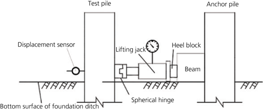
Schematic diagram of lateral pile load tests performed at the site (Xi and Ma, 2017)
General stratigraphy at the location of pile 1
| Start depth: m | End depth: m | Soil/rock type | SPT N value | Unconfined compressive strength: MPa | Elastic modulus, E′: MPa | Friction angle: ° | Cohesion: kPa |
|---|---|---|---|---|---|---|---|
| 0.0 | 1.0 | Medium dense sand | 15 | — | 15 | 31 | — |
| 1.0 | 3.0 | Very dense sand | 50 | — | 50 | 41 | |
| 3.0 | 9.5 | Siltstone | — | 1.5 | 200 | 35 | 80 |
| 9.5 | 30.0 | Conglomerate | — | 2.0 | 250 | 35 | 100 |
General stratigraphy at the location of pile 2
| Start depth: m | End depth: m | Soil/rock type | SPT N value | Unconfined compressive strength: MPa | Elastic modulus, E′: MPa | Friction angle: ° | Cohesion: kPa |
|---|---|---|---|---|---|---|---|
| 0.0 | 1.5 | Very dense sand | 50 | — | 50 | 41 | — |
| 1.5 | 5.0 | Very dense sand/sandstone | — | 0.5 | 70 | 22 | 29 |
| 5.0 | 10.0 | Conglomerate | — | 2.5 | 100 | 30 | 70 |
| 10.0 | 18.5 | Conglomerate/siltstone | — | 2.0 | 80 | 30 | 65 |
| 18.5 | 30.0 | Calcisiltite | — | 3.0 | 80 | 27 | 70 |
Lateral pile analysis methodologies
Commonly adopted methods used for lateral load capacity calculations for piles – namely, the Broms method and p–y non-linear analyses – were part of this study. With recent advancements in computing capabilities, finite-element analysis is also adopted by geotechnical engineers for lateral load capacity calculations and was made part of this study. The background of these methods along with their applicability to the current situation, as well as the results obtained, are discussed in the next sections.
Broms method
This method (Broms, 1964b), although developed to estimate the lateral resistance of piles in sands, can be used to predict the lateral deflection of piles at the ground surface. It was developed under the assumption that the ultimate lateral resistance of a short pile is governed by the passive earth pressure of the surrounding soil, whereas for piles with large penetration depths it is majorly governed by the yield resistance. The linear elastic approach is a key concept in this method, wherein the load is approximately between 0.3 and 0.5 times the ultimate load. Although this methodology is very useful for quickly designing a pile, it is not very reliable since the pile–soil interaction is assumed to be linearly elastic. Also, this method was developed for piles completely embedded in sand. In the current scenario, where the piles are rock socketed (generally observed in Dubai, UAE), the designer needs to take the weighted average of the profile or assume an equivalent sand profile over the critical depth for the lateral load analysis. As this is very much dependent on the designer’s assumption and choice of friction angle, results obtained using this method could be highly conservative and non-representative. Using engineering judgement and the weighted average approach, friction angles of 35 and 40° were respectively used for pile 1 and pile 2. On performing calculations, lateral deflections at the ground level were found to be 50.95 and 42.46 mm for pile 1 and pile 2, respectively, which are very high compared with those obtained from pile load tests (6.64 mm for pile 1 and 5.62 mm for pile 2). As field test data are not available in all projects, these calculated higher magnitudes of lateral deflections will undoubtedly lead to the designer tending to increase the pile diameter, which will increase the construction cost.
p–y non-linear analysis
The Lpile software was used to perform p–y non-linear analyses. For modelling of the lateral response of sand, the p–y curve developed by Reese and Van Impe (2011) and the American Petroleum Institute (API) was utilised. The p–y response curve available for weak rock in the Lpile software was utilised to model the rock layers. In p–y non-linear analysis, the soil resistance is modelled as non-linear springs. It involves replacing soil around the pile by a set of mechanisms that indicate that the soil resistance ‘p’ is a non-linear function of the pile deflection ‘y’. An iterative technique is used to evaluate deflections and moments until the soil resistance and load (depending on the deformation of the pile) are in equilibrium. The p–y curves for sand proposed by Reese and Van Impe (2011) and API do not have a significant difference in the ultimate resistance. However, the API model uses a hyperbolic tangent function for computation. The main difference between the two methods is the initial modulus of subgrade reaction and the shape of the curves. For piles socketed in rock, each layer was modelled differently in the p–y non-linear analysis approach. It should be emphasised that the p–y curve for the rock is generated using the option of weak rocks in the Lpile software. On performing calculations with the p–y curve for sand as per Reese and Van Impe (2011), deflections at the ground level were found to be 45.81 and 26.5 mm for pile 1 and pile 2, respectively. With the p–y curve for sand based on the API model, lateral pile deflections at the ground level were calculated as 31.28 and 19.81 mm. Although both methodologies undoubtedly resulted in higher magnitudes of lateral deflection compared with those from pile load tests (6.64 mm for pile 1 and 5.62 mm for pile 2), the p–y curve based on sand developed by API was noticed to be less conservative. However, it should be clearly emphasised that p–y curves developed for sand are based on lateral load tests performed on piles with specific ground conditions.
Finite-element analysis using the Plaxis 3D software
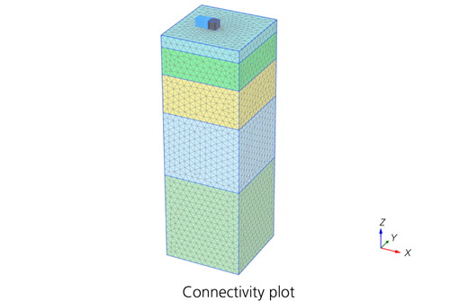
Three-dimensional (3D) finite-element analysis (Figure 2) was carried out through the Plaxis 3D software using the inputs shown in Tables 1 and 2. Finite-element mesh was generated using ten-noded tetrahedron elements. A fine mesh option was selected in the Plaxis auto meshing tool. The model size and boundary conditions were selected in such a way that there is no effect of boundary conditions on the analysis. The vertical boundaries of the model were restrained for any horizontal movement, whereas the base of the model was restricted for both horizontal and vertical movements. However, the top of the model was unrestrained. Load was defined as pressure load applied in increments similar to a pile load test. Two material models – namely, the Mohr–Coulomb (MC) material model and hardening soil model with small-strain stiffness (HSS) – were used for analysis, using the Plaxis software to simulate the soil behaviour.
The material model most commonly adopted by design engineers is the MC material model because limited data are available to designers in the initial phase of design. Analysis was performed using the MC model, which considers soil behaviour as linear elastic-perfectly plastic, for both sand and rock. This model assumes that soil resistance increases linearly with displacement until the failure criterion determined by the MC model is reached.
For modelling the non-linear behaviour of the ground, the constitutive model used in the analysis was the HSS model, which is a modification of the hardening soil model that considers the increased stiffness of soils at small strains. At low strain levels, most soils exhibit a higher stiffness than at engineering strain levels, and this stiffness varies non-linearly with strain. As the stiffness modulus can change according to the strain levels, this model shows the non-linear elastic characteristics of soil. The HSS material model was used to model sands, and the MC model, rocks. This material model requires additional stiffness parameters (Table 3), and these were derived using standard correlations based on SPT N values. These additional parameters considered for sand layers for the soil profile at pile 1 and pile 2 were derived based on the following assumptions.
The secant modulus (E 50) was derived from Tables 1 and 2 using E 50 ≈ E′.
The oedometer modulus (E oed) was calculated based on Hooke’s law:
1where ν is Poisson’s ratio.
The loading/unloading stiffness (E ur) was conservatively selected as three times E 50, based on the Plaxis manual (Bentley Systems, 2017). This ratio ranges between 3 and 6 (Obrzud and Truty, 2018).
The small-strain stiffness (G 0) was calculated using , where ρ is the density of the soil and V s is the shear wave velocity for the soil layer calculated based on SPT as V s = 125 × N 0.3 based on the paper by Okamoto et al. (1989).
Additional stiffness parameters required for modelling sand layer using the HSS material model
| Soil profile (pile number) | Soil layer | E 50: MPa | E oed: MPa | E ur: MPa | G 0: MPa |
|---|---|---|---|---|---|
| Pile 1 | Medium dense sand | 15 | 20 | 45 | 154 |
| Very dense sand | 50 | 67 | 150 | 317 | |
| Pile 2 | Very dense sand | 50 | 67 | 150 | 317 |
Note: for input in the Plaxis software, the above values were corrected for reference pressure (p ref) = 100 kPa
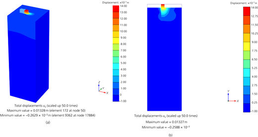
On completing numerical analyses, lateral deflections of the pile at the ground level using MC material were calculated to be 23.6 and 15.89 mm (Figure 3) for pile 1 and pile 2, respectively. The lateral pile deflections at the ground level using the HSS material model were 16.95 and 13.30 mm (Figure 4) for pile 1 and pile 2, respectively.
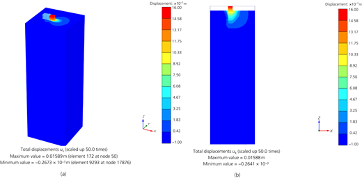
Lateral deflection of pile 2 using the MC model: (a) 3D view; (b) two-dimensional (2D) view
Lateral deflection of pile 2 using the MC model: (a) 3D view; (b) two-dimensional (2D) view
Comparison of analyses and discussion
On performing the analyses with various approaches, the results obtained are summarised in Tables 4 and 5 for pile 1 and pile 2, respectively. For better understanding, these values are graphically presented in Figures 5 and 6 for pile 1 and pile 2, respectively. It is evident from all results that the lateral deflection values obtained from field tests are small compared with those from the adopted methodologies. This confirms the importance of field tests in geotechnical engineering practice, which rule out most assumptions and yield values that are more realistic and not conservative. However, it is not possible to conduct field tests in all projects, and hence empirical/numerical calculations cannot be ruled out. However, it is the responsibility of the designer to choose wisely a suitable calculative method that gives results close to reality. Within the methods used as part of this research work, the Broms method was found to be very conservative. On the other hand, lateral deflections obtained from finite-element analysis (although not being very close to field test values) are lower compared with those from other methods, and this helps the designer optimise the pile diameter. It should be emphasised that the HSS model has given less conservative values compared with the MC model.
Lateral deflections using different methods for pile 1
| Load: kN | Lateral deflection of the pile: mm | |||||
|---|---|---|---|---|---|---|
| Broms method | Reese method (using Lpile software) | API method (using Lpile software) | 3D finite-element analysis (using MC for sand) | 3D finite-element analysis (using HSS for sand) | Field test | |
| 0.00 | 0.00 | 0.00 | 0.00 | 0.00 | 0.00 | 0.00 |
| 106.00 | 13.33 | 3.00 | 3.00 | 4.90 | 2.65 | 0.61 |
| 206.00 | 25.91 | 11.72 | 10.33 | 10.70 | 6.76 | 1.60 |
| 305.00 | 38.37 | 22.22 | 17.54 | 16.90 | 11.42 | 3.69 |
| 405.00 | 50.95 | 45.81 | 31.28 | 23.60 | 16.95 | 6.64 |
Lateral deflections using different methods for pile 2
| Load: kN | Lateral deflection of the pile: mm | |||||
|---|---|---|---|---|---|---|
| Broms method | Reese method (using Lpile software) | API method (using Lpile software) | 3D finite-element analysis (using MC for sand) | 3D finite-element analysis (using HSS for sand) | Field test | |
| 0.00 | 0.00 | 0.00 | 0.00 | 0.00 | 0.00 | 0.00 |
| 106.00 | 11.11 | 1.11 | 1.12 | 3.00 | 1.80 | 0.52 |
| 206.00 | 21.60 | 6.19 | 5.67 | 6.60 | 4.76 | 1.28 |
| 305.00 | 31.97 | 12.33 | 10.37 | 11.00 | 8.50 | 3.24 |
| 405.00 | 42.46 | 26.50 | 19.81 | 15.89 | 13.30 | 5.62 |
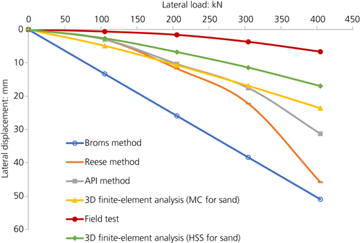
Variation of lateral deflection with lateral load for pile 1 using different methods
Variation of lateral deflection with lateral load for pile 1 using different methods
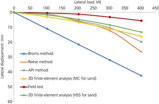
Variation of lateral deflection with lateral load for pile 2 using different methods
Variation of lateral deflection with lateral load for pile 2 using different methods
Conclusions
After performing various analyses and observing the magnitudes of lateral deflections of piles obtained from field tests, conclusions and recommendations are summarised as follows.
Stiffness and strength parameters for sand used in pile capacity calculations were based on the SPT N value using standard correlations, and results were found to be underestimating the actual capacities, leading to overdesign.
The applicability of the Broms method to rock-socketed piles with the assumption of a weighted soil profile is not accurate and will lead to uneconomical design of piles.
At smaller lateral loads, p–y non-linear analysis and finite-element approaches predict the lateral response of soil more accurately compared with the Broms method.
Finite-element analysis using the MC model gives less deflection at higher loads, but using a single value of stiffness overestimates the deflection at lower loads.
The HSS model predicts behaviour better, as it is able to simulate stiffness modulus change according to the strain levels. Compared with other methods, the final settlement and the displacement curve obtained are more representative of the results obtained from field tests.

