Design of humanitarian supply chain system by applying the general two-stage network DEA model

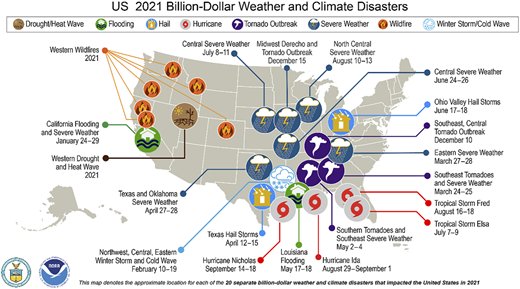
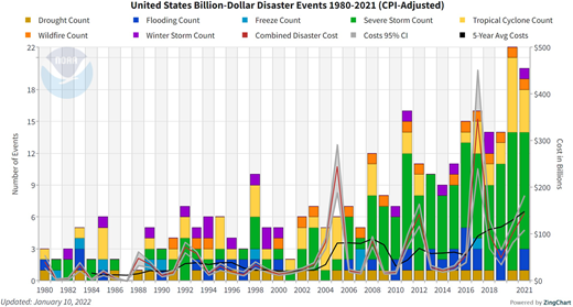
The humanitarian supply chain network (HSCN) plays a critical role in providing disaster relief items such as medicine, drinking water, food and daily commodities to alleviate people's suffering. The year 2017 became a historic year of weather and climate disasters for the United States, which, in total, was impacted by 16 separate billion-dollar disaster events, including three tropical cyclones, two inland floods, eight severe storms, a crop freeze, drought and wildfire. In early 2019, Alaska, the coldest state in the US, posted its warmest March on record by a landslide and the powerhouse storm in the central US became the second billion-dollar weather disaster of 2019. The year 2020 set the new annual record of 22 events, breaking the previous record of 16 events in 2011 and 2017. During 2020 and 2021, the US experienced a very active year of weather and climate disasters (see Figure 1), including the COVID-19 pandemic. According to the data developed by the NOAA's National Climatic Data Center, the US, on average, faces ten severe weather events yearly exceeding one billion dollars in damage (see Figure 2). A comparison with an annual average of only two such events throughout the 1980s clearly may force us to speculate that a warming climate could make these disasters more frequent and intense. In this respect, an HSCN design has become an important strategic decision due to the significant damage inflicted by several natural disasters (Petrudi et al., 2020). Moreover, COVID-19 and its variants have brought issues of emergency relief planning through the HSCN again.

The HSCN is defined as the flow of relief aid and related information between people from disaster-stricken areas and donors to alleviate the suffering of vulnerable people. Indeed, after emergencies, it is critical for emergency response facilities (ERFs) to distribute humanitarian aid to the affected areas efficiently and effectively to save human lives and alleviate suffering and rapid recovery. Van Wassenhove (2006) emphasizes that since disaster relief is 80% logistics, it would follow that the only way to operate the HSCN system efficiently and effectively is through efficient, effective and slick logistics operations, and more precisely, supply chain management. Logistics planning in emergencies involves the quick and efficient distribution of emergency supplies from the ERFs to the affected areas via supply chains. Several authors (Boonmee et al., 2017; Cao et al., 2018; Hong and Jeong, 2019; Petrudi et al., 2020; Sarma et al., 2020) have considered various HSCN design models. Zhang et al. (2019) and Liu et al. (2019) have reviewed the papers on the HSCN design problems. Gress et al. (2021) present a methodology for designing an HSCN to distribute COVID-19 vaccines in Mexico. Malmir and Zobel (2021) propose a sustainable HSCN design model considering the COVID-19 outbreak.

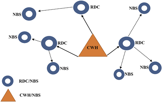
The ERFs considered in this paper are three distinctive ones. They are (1) central warehouses (CWHs) or distribution warehouses, where emergency relief commodities are stored, (2) intermediate response facilities termed relief distribution centers (RDCs) or commodity distribution points and (3) neighborhood sites (NBSs), which are affected areas in need of humanitarian items. These ERFs are depicted in Figure 3 by modifying Habib et al. (2016).

As mentioned above, an HSCN design problem is inherently strategic and long-term. The main objective of the strategic level is to strengthen emergency preparedness as well as to select the most cost/distance-effective location of CWHs and RDCs among a set of candidate locations, to establish the distribution of emergency supplies throughout the HSCN and to assign NBSs to RDCs and RDCs to CWHs. Making such a decision is a critical area in designing an effective HSCN. However, traditional cost-based facility location-allocation models implicitly assume that located facilities will always be in service or available and do not consider an associated risk of disruption. But all facilities are susceptible to natural/weather disasters, strikes, or pandemics. A lack of flexibility and interdependency in the HSCN could aggravate the effects of disruptions. Snyder et al. (2016) review nearly 150 articles related to the OR/MS literature on supply chain disruptions to take stock of the research and provide an overview of the research questions. They predict that the literature on supply disruptions will continue to increase over the coming years, identifying seven topics as avenues for future research. Li et al. (2020) investigate supply chain network characteristics that can better understand supply chain resilience under disruption risk propagation. Aldrighetti et al. (2021) review more than 220 articles on the quantitative models of supply chain network design under disruption risks in industrial supply chain management and logistics, highlighting drawbacks and missing aspects in the related literature and discussing future research directions. Ganesh and Kalpana (2022) point out that though the research on supply chain risk management (SCRM) remains for an extended period; industries still face difficulties managing supply chain risks. Also, supply chain managers have begun to focus on decision-making based on numerous data sources for predicting uncertainties more accurately to achieve a proactive and predictive intelligent risk management mechanism. These characteristics make artificial intelligence (AI) and machine learning (ML) suitable SCRM techniques. Emphasizing that these AI techniques are in an emerging stage in SCRM, they (2022) provide unexploded and missing aspects in current research, challenge on implementing AI technologies and describe promising avenues for the future after reviewing 127 papers on SCRM.

The typical multi-objective programming model allows the decision-maker to decide weights for the objective function's deviational variables. It mainly reflects the importance and desirability of deviations from the various goals. However, the actual efficiency of the resulting HSCN is not known. Ragsdale (2018) states that there is no standard procedure for assigning values to the weight factors to guarantee finding the most desirable solution. He suggests that it will be necessary for the decision-makers to follow an iterative procedure. Decision-makers could try a particular set of weights, solve the problem, analyze the solution and then refine the weights and solve it again. He concludes that it is essential for the decision-makers to repeat this process several times to find the most desirable solution. Thus, it is unavoidable for decision-makers to use some of their subjective judgment.

Then, a challenging question is how the best alternative option can be selected if the most desirable solution is different among the decision-makers. It would be imperative to evaluate the efficiency of all alternatives generated by the model and select the most desirable one(s) with an optimized objective function or without any subjective judgment. Following this vein, Hong and Jeong (2019) apply a single-stage network data envelopment analysis (SSN-DEA) method for evaluating the various HSCN schemes generated by solving the multi-objective programming models formulated for the HSCN design problem.

For the SSN process, the conventional DEA (C-DEA) method proposed by Charnes et al. (1978) has been widely accepted as an effective performance evaluation tool for assessing the relative efficiency of a set of peer entities called decision-making units (DMUs). C-DEA determines which DMUs make efficient use of their inputs and produce most outputs and which do not. Thus, the C-DEA model classifies DMUs into two groups, i.e. separating efficient DMUs from inefficient DMUs, using efficiency score (ES). The analysis indicates where an inefficient DMU might look for benchmarking help to search for ways to improve. Each DMU is evaluated with its most favorable weights due to the DEA's nature of self-evaluation, ignoring unfavorable inputs or outputs to raise self-efficiency. As a result, C-DEA's critical weakness of a lack of discrimination is caused because it classifies a considerable number of DMUs out of the set of DMUs as efficient, with an ES equal to 1.

Sexton et al. (1986) propose a cross-evaluation concept to do the peer evaluation rather than the C-DEA's pure self-evaluation to remedy this deficiency. Doyle and Green (1994) suggest a cross-evaluation matrix for ranking the units by applying the cross-efficiency DEA (CE-DEA) model. Generally, the CE evaluation can provide a full ranking for the DMUs. But, as Doyle and Green (1994) find, the non-uniqueness of cross-efficiency scores (CESs) and non-consistent rankings have been critical issues for applying the CE-DEA. Another concept for peer evaluation is the super-efficiency DEA (SE-DEA), which is introduced to compensate for the weaknesses of C-DEA and CE-DEA. A DMU under evaluation is excluded from the DEA models' reference set. The resulting model is called a SE-DEA model that has significance for discriminating among efficient DMUs. Charnes et al. (1992) use the SE model to study the efficiency classification's sensitivity. Anderson and Peterson (1993) propose the SE model to rank the efficient DMUs. But the critical issue of using the model is that the adjacent DMUs decide the super efficiency score (SEC) of an efficient DMU, so it would be awkward for DMUs to be ranked by the SESs.

As big data research becomes an essential area of operations analytics, DEA has evolved into a tool for big data analysis. As Cook and Zhu (2014) mention, an important development area in the DEA applications has been devoted to applications wherein DMUs represent network processes. In fact, a network DEA has been significant steam that controls efficiencies of various sub-stages in a complex structure. A substantial body of DEA research has focused on the network DEA since the network DEA can satisfy three defining properties of big data, volume, variety and velocity (Zhu, 2022). DMUs may consist of two or more stage network structures with intermediate measures. Monfared and Safi (2013) state that the SSN-DEA model considers a DMU as a “black box” and neglects intervening processes, i.e. different series or parallel functions. Thus, the “black box” approaches for the single-stage process provide no insights regarding the inter-relationships among the components' inefficiencies and cannot offer specific process guidance to DMU managers to improve DMU's efficiency.

Out of the literature on the optimization models for HSCN, Hong and Jeong (2019) consider four performance measures simultaneously using the multi-objective programming (MOP) model. Then, they apply the SSN-DEA method to find the efficient configurations out of the various HSCN configurations generated by the MOP model. Their work (2019) would be the first attempt to combine the MOP model with the SSN-DEA method in the literature on the design of HSCN. Monfared and Safi (2013), Cook and Zhu (2014) and Zhu (2022) state the strengths of the TSN-DEA in contrast to the weaknesses of the SSN-DEA.

Many authors have considered the single-stage HSCN design problem using multi-objective programming models. Single-stage network DEA (SSN-DEA) models have recently been applied to evaluate the efficiency of designed HSCN schemes. As mentioned, the SSN-DEA methods show several intrinsic weaknesses, such as ignoring the intervening processes and producing inconsistent rankings. The SSN-DEA model's most critical weakness lies in its inconsistent efficiency score (ES), which depends on the DMUs under evaluation in the reference sets. For example, the top-ranked DMU based on the ESs when all DMUs are evaluated should maintain the top-ranking position even though some lower-ranked DMUs are not assessed together. But the SSN- DEA models frequently allow the previously lower-ranked DMU to overtake the top-ranked DMU to become a new #1 DMU if some lower-ranking DMUs are not evaluated together. Thus, the research questions on the SSN-DEA's weaknesses have been raised by various authors.

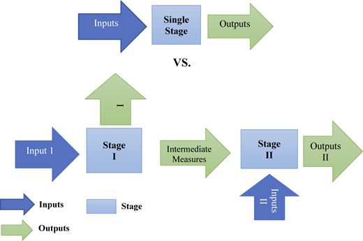
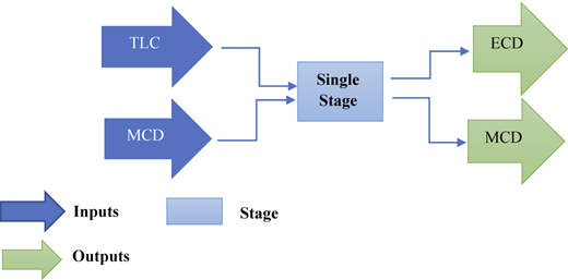
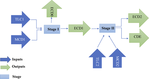
There is a research gap in evaluating DMUs with a single-stage network process since, as mentioned above, SSN-DEA methods do not consider the intervening processes. Moreover, these SSN-DEA methods do not rank the efficient DMUs consistently. Thus, the research question is how to transform the single-stage HSCN system into a general two-stage network (GTSN) process system so that GTSN-DEA (GTSN-DEA) model is applied to compensate for the weaknesses of the SSN-DEA models for the HSCN design problem. To answer these questions, this paper proposes transforming a single-stage HSCN design problem into a two-stage network (TSN) process to apply the GTSN-DEA model. See Figure 4, depicting the SSN-GTSN-DEA structures. We identify efficient HSCN configurations among the schemes generated by solving the WGP model for various weight set values for the transformed TSN process. Using the case study, we demonstrate that the proposed approach shows a better analysis of the efficiency of the designed HSCN configurations and produces more consistent and robust rankings after evaluating efficient HSCN configurations. Thus, the contribution of this paper is to reveal the could-be hidden network schemes, if SSN-DEA is only applied, that the decision-makers would not consider as the candidate schemes for their final decision.

The proposed two-stage network design problem differs from the two-stage stochastic programming model with the high uncertainty in the decision environment, such as uncertainty of inputs and outputs at each stage. The paper considers a decision environment with no uncertainty, such as given inputs and outputs. After GTSN-DEA is applied, an additional research question is how to investigate whether the GTSN-DEA ranks the top-rated DMUs more consistently. In fact, this study would be the first attempt to answer these kinds of research questions for the HSCN design problem in a pre-disaster scenario, which consists of finding the optimal ERFs under the risk of facility disruption.

The following nomenclature is used throughout the paper to formulate a multi-objective mathematical model (see Hong and Jeong, 2019):

The first goal is minimizing the related logistics costs, which is the traditional objective of most FLA models. Given this problem set, the total logistics cost (TLC) consists of the expenses for CWHs (construction, operation and distribution of items from CWHs to RDCs) and the costs for RDCs (building and development as well as distribution of relief items from RDCs to NBSs):

The next goal is related to the demand-oriented objective, which focuses on measuring the “closeness” of the ERFs. In other words, ERFs should be located at a place close to the covered sites to deliver the relief item as quickly as possible. The second goal is to minimize the maximum coverage distance (MCD) such that each NBS is covered by one of the RDCs, and each RDC is covered by one of the CWHs within the endogenously determined distance. This goal minimizes the longest delivery distance between CWHs and RDCs, and RDCs and NBSs. As the MCD increases, it will cause ineffectiveness to the resulting HSCN. Now, MCD is given by

The ERFs should be located at the least likely locations to be disrupted to enhance supply chain resilience to inevitable disasters. The third goal related to the least likely locations to be disrupted is to maximize the expected amount of covered demands (ECD) by the ERFs, which is expressed as

where

• $pj−$ the probability that the RDC_j is disrupted (or risk probability);

• $qi−$ the probability that the CWH_i is disrupted (or risk probability).

In case of emergency, each resident should be within a certain distance of the nearest centers to be served. Also, some environmental difficulties or constraints, such as weather issues and road damage, may limit the maximum coverage distance of MCD in (2). Thus, the maximum effective coverage distance in case of emergency, denoted by $Dc$⁠, would be shorter than MCD. In addition, it is desirable to maximize the covered demands within $Dc$⁠, while minimizing MCD. The next goal is to maximize the covered demands in case of emergency, CDE, which is expressed as

where an indicator parameter, $κjg$⁠, is

Let the nonnegative deviation variables, $δTLC+,δMCD+,δECD−,andδCDE−,$ represent the amounts by which each value of TLC, MCD, ECD and CDE deviates from the target values. Using α = {α₁, α₂, α₃, α₄} and $∑κ=14ακ=1$ denote relative weights attached to the corresponding goal, the following weighted goal programming (WGP) model can be formulated:

subject to

Constraints (11) define the upper bound of the number of CWHs that can be built. Here at most $Wmax$ is allowed. Constraints (12) ensure that the potential CWH location will not be selected simultaneously as both CWH and RDC. Constraints (13) ensure that if a potential CWH location i is not selected $(i.e.,Wi=0),$ its demand must be satisfied by an RDC or a CWH. Constraints (14) make certain that each NBS (⁠$n∈N$⁠) is assigned to either an RDC or a CWH. Constraints (15) limit the minimum and maximum number of RDCs to be covered by each CWH. Constraints (16) ensure that CWHs only supply the selected RDCs. Constraints (17) limit the total number of selected RDCs to be less than or equal to a user-specified number, $Cmax$⁠. Constraints (18) ensure that NBSs or unselected CWH locations can only be assigned to the selected candidate RDCs. Constraints (19) ensure that the chosen candidate RDC_j must cover a minimum number of $lj$ NBSs and can only cover a maximum of $Lj$ NBSs. Constraints (20) and (21) show the shipping capacity of RDCs and CWHs, respectively. Solving the above WGP model in (6)–(21) for a given set of weights would generate an HSCN network scheme. Thus, by changing the weight set, various HSCNs could be developed. Each network scenario could be treated as a DMU for the DEA method to be applied to evaluate all scenarios with two inputs, TLC and MCD and two outputs, ECD and CDE.

As shown in Eq. (6), the objective function of WGP is to minimize the weighted sum of the percentage deviations. The above WGP model is an extension of the GP model, whose objective is to minimize the sum of the deviations. The above weighted GP model differs from the epsilon $(ε)$ multi-objective optimation method, where one objective will be used as the objective function, and the remaining objectives will be used as constraints using the epsilon. Lexicographic GP is another version of GP when a specific goal is strictly preferable to the other goals, or the decision maker has a clear preference order for achieving the goals.

First, as shown in Figure 5, the SSN model is applied. DMUs, equivalent to the HSCN schemes generated by solving the WGP model for different weight values assigned to each goal, can be evaluated by applying the DEA method. The mathematical model of the SSN-DEA model for DMU_ω, is given by

subject to

where u_r is a weight or coefficient assigned by DEA to output r, and v_i is the weight or coefficient assigned by DEA to input i. Let $θω*,$ efficiency score (ES), represent the optimal value of the objective function in (22) corresponding to the optimal solution (u*, v*). DMU_ω is said to be efficient with $θω*$ of 1.

The CE-DEA method consists of two phases. The first phase is self-evaluation, where DEA scores are calculated using the model by (22)–(24). In the second phase, the weights arising from the first phase are applied to all DMUs to get the cross-efficiency score (CES) for each DMU. Let $Eωω$ represent the DEA score for DMU_ω and $urω*$ and $viω*$ denote the optimal solution obtained from solving (22)–(24). Now, the cross efficiency of DMU_j using a rating DMU_ω is

By averaging $Ejω$ in (25), the CES of $DMUω$ is given by

A super-efficiency DEA (SE-DEA) would generate a super-efficiency score (SES) obtained from the C-DEA model after a DMU under evaluation is excluded from the reference set. Thus, the SESs of efficient DMUs can have higher values than 1, the maximum value of the ES obtained by other DEA methods. The SE-DEA model is given by

subject to

The SSN model can be decomposed into an equivalent GTSN model, as shown in Figure 6. In other words, an HSCN network scheme is decomposed into two stages, i.e. stage 1 represents the flows from CWHs to RDCs, while stage 2 represents the flows of items from RDCs to NBSs. The two inputs, TLC and MCD, are split into TLC1 and MCD1 for stage 1 and TLC2 and MCD2 for stage 2, respectively. An output ECD is divided into ECD0 and ECD1 for stage 1 and ECD2 for stage 2. The ECD0 denote the ECD for the sites where CWHs are located, while ECD1 becomes an intermediate measure that flows from stage 1 to stage 2. Now, the split inputs and outputs are expressed as

where the expression of ECD is given in (4). Since each stage in Figure 4 works together to achieve the best performance of the HSCN, a centralized model is applied to analyze the converted two-stage network.

where $θω1$ and $θω2$ are ESs of stages 1 and 2 for DMU_ω, respectively, and the weights for each input, output and intermediate one are ${v1,v2,Q1,Q2,λ1,u1,u2,η1}≥0.$ Now, the overall centralized ES, $θωcen$⁠, can be given by:

subject to

Let $θω1max$ be the maximum efficiency score of stage 1, then the following LP model for the model in (39)–(41) is formulated:

subject to

From (42)–(45), the optimal value of (42), an estimator $θω1$ for the first stage, is a variable whose maximum value is $θω1max$⁠. Now, the overall (centralized) ES for the two-stage model, $θωcen*$⁠, is a function of $θω1$ and can be formulated as

subject to

Li et al. (2012) propose an iteration method by setting $θω1=θω1max−z∆ε$⁠, where $∆ε$ is a step size and $z=0,1,2,…,zmax+1$⁠, $zmax≤[θω1max∆ε].$⁠. The optimal global efficiency of the system under evaluation is estimated as $θωcen*=maxzθωcen,1(z)$⁠. Now the formal procedure can be stated as follows:

Procedure

1. Step 1: [Identifying efficient DMUs for SSN-DEA Model]

   • Using the m-DEA method, evaluate all DMUs by solving an LP given in (22)–(24).

   • Identifying efficient DMUs where their ESs are equal to 1, $θω=1$ and stratify them into a set $G1$⁠.

   • Using (25)–(26) and (27)–(29), obtain the CESs and SESs for the DMUs in $Θ1$ and rank them based on these two ESs.

2. Step 2: [Decomposing and Applying GTSN-DEA Model]

   • For DMUs in $Θ1$⁠, decompose the SSN model into a GTSN model.

   • Setting $θω1=θω1max−z∆ε$⁠, $z=0,1,2,…,zmax+1$⁠, $zmax≤[θω1max∆ε]$⁠, set $θωcen*=maxzθωcen,1(z)$⁠.

   • Rank the DMUs in $G1$ based on $θωcen*$ in (v).

A case study uses major disaster declaration records in South Carolina (SC). We cluster forty-six (46) counties based on proximity and populations into twenty (20) counties. Then, one location from each clustered county based on a centroid approach is chosen by assuming that all population within the grouped county exists in that location. Federal Emergency Management Agency (FEMA) database shows that SC has experienced sixteen (16) major natural disaster declarations, such as tornadoes, hurricanes, floods, etc., from 1964 to 2017. The database also lists counties where a major disaster was declared. This paper assumes that the county's emergency facility is disrupted and shut down when a major disaster is declared. Based on the historical record and the assumption, each neighborhood's risk probability (a county or a clustered county) is calculated in Table 1 by dividing the years with major natural disasters by the total years. The five potential locations for CWHs are selected based upon population, the proportion of area that each site would potentially cover and the proximity to Interstate Highways in SC.

The number of RDCs and CWHs to be built are pre-specified in most cases. We simplify the TLC function given by Eq. (1) by excluding the fixed cost terms for RDCs and CWHs. If the actual data are available for the fixed cost terms, we can readily lift such restrictions to obtain more revealing results. Also, the following parameters are pre-determined for our case study. The maximum numbers of RDCs and CWHs that can be built, $Cmax$ and $Wmax$⁠, are set to 5 and 2, respectively. The minimum and maximum number of RDCs that a CWH must handle, $ki$ and $Ki$⁠, are set to 1 and 10, respectively. Each RDC must handle at least 2 (⁠$ℓj=2$⁠) and at most 7 (⁠$Lj=7$⁠) NBSs. The capacities of RDCs and CWHs, $CAPjmax$ and $CAPimax,∀jand∀i$⁠, are set to 1,500 K and 2,500 K in terms of the number of humanitarian items.

The WGP model is solved for various values of weight, $α={α1,α2,α3,α4}$⁠. Each weight alters between 0 and 1 with an increment of 0.1, subject to $∑κ=14ακ=1$⁠. We use the 'Gurobi' Solver Engine of Analytic Solver software. Two hundred eighty-six (286) configurations arising out of the combinations of the setting of $α$ are solved on an Intel® Xeon ® Gold 5122 HP Z4 Workstation PC (2 processors) with 32 GB of RAM installed using a 64-bit version of Windows 10. It takes 10,238 s (approximately 2.84 h) to solve all 286 sets of the GP model. On average, it takes 35.8 s to solve one weight set of the GP. The 286 configurations are reduced to sixty-eight (68) consolidated structures since several cases yield the same values of the four-performance metrics. Each of the 68 configurations is considered a DMU, representing the optimal locations and allocations of ERFs.

As Step 1 in the procedure proposes, we apply the C-DEA model in (22)–(24) for the SSN, as shown in Figure 5, to find efficient DMUs with a perfect ES of 1.000. Twenty-six (26) DMUs with ES equal to 1.000 identified from the 68 consolidated DMUs are reported in Table 2, as the ES in the last column indicates. Using Eqs (30)–(36), we decompose the inputs and outputs of those 26 efficient DMUs (see Figure 6) and also list them in Table 2, starting with TLC1 from the 3rd column. Now, we apply CE- and SE-DEA of the SSN-DEA to compute the cross-efficiency score (CES) and super-efficiency score (SES) for each efficient DMU. We also apply the GTSN-DEA in Step 2 using the decomposed inputs and outputs listed in Table 2. These efficiency scores for the SSN- and GTSN-DEA are reported in Table 3 where $θω1$ and $θω2$ denote ESs of stages 1 and 2, respectively, and the overall centralized ES, $θωcen$⁠, are reported along with the corresponding rank, [R], based on each efficiency score. Table 3 shows that each approach finds a different DMU as the top-ranked one. DMU₁₃₃ and DMU₈₇ are ranked #1 by CES and SES, respectively, for the SSN-DEA model. The GTSN-DEA ranks DMU₁₇₄ as #1, based on the overall efficiency, $θωcen*$⁠. We observe that DMU₁₃₃, ranked #1 by CES, is surprisingly ranked #4 and #17 by SES and $θωcen*$⁠. We also note that DMU₈₇, ranked #1 by SES, is ranked #17 and #26 by the other two methods. The GTSN's #1 ranked DMU₁₇₄ is ranked #24 and #3 by CES and SES.

Table 2 compares these three top-ranked DMUs and shows each DMU has dominating inputs or outputs. For example, DMU₈₇ with a perfect ES, i.e. $θ872=1,$ at stage 2, as shown in Table 3, has the smallest two inputs to stage 2, TLC2 and MCD2, and the greatest output from stage 2, CDE, whereas DMU₁₇₄, with a perfect ES, $θ1741=1$ at stage 1, has the smallest two inputs to stage 1, TLC1 and MCD1, and the greatest outputs, ECD0, ECD1 and ECD2, but the lowest CDE among these three top DMUs. Inputs and outputs for DMU₁₃₃ ranked #1 by CES, are listed between the other two top-ranked DMUs, DMU₈₇ and DMU₁₇₄.

To investigate the robustness of ranks generated by each method, we select eighteen (18) DMUs out of twenty-six (26) efficient DMUs shown in Tables 2 and 3 These 18 DMUs ranked at least #9 by any efficiency score are evaluated and reported in Table 4. For comparison purposes, besides the new ranking, [R], based on the current efficiency score, the expected ranking, E[R], based on the rankings in Table 3, where 26 DMUs are ranked, is also reported in Table 4. For example, DMU₈₇, ranked #17 among 26 DMUs by CES, shown in Table 3, is expected to be ranked #14 for the selected 18 DMUs. For comparison between [R] and E[R], the absolute rank difference (ARD) between these two ranks, ARD = |[R] – E[R]|, is computed to measure each method's rankings' robustness and is also reported in Table 4. For example, DMU₈₇, whose expected rank is #14 out of 18 DMUs, turns out to be #16, so its ARD is 2. Table 4 shows that the CES finds DMU #81 a new top-ranked one out of 18 DMUs, initially ranked #3 among 26 efficient DMUs, while the SES ranks DMU₂₀₅ as a new top-ranked one, which is expected to be ranked #11. In addition, the columns of ARDs of CES and SES under the SSN-DEA model exhibit the DEAs' critical weakness, i.e. the inconsistency of ranking DMUs. Out of 18 DMUs, the CES and SES generate 14 DMUs and 17 DMUs with positive ARDs, respectively, with a maximum ARD of 14. In contrast, the proposed GTSN-DEA finds the same ranks for 9 DMUs, including the top-three DMUs, DMU₁₇₄, DMU₁₈₀ and DMU₁₄₃. Table 5 reports each approach's total ARD, mean ARD and maximum ARD. The results shown in Table 5 assert that the proposed GTSN-DEA method dominates in all three measures and generates more consistent and robust rankings than the two approaches, CES and SES, of the SSN-DEA.

For further investigation, eleven (11) DMUs ranked at least #5 by any efficiency scores are selected, evaluated and reported in Table 6. The results of ARDs in Table 6 are summarized in Table 7, just like Tables 4 and 5 The CES continues to rank DMU₈₁ again as a top-ranked one, while the SES, which ranks DMU₂₀₅ No. 1 with 18 DMUs under evaluation, surprisingly identifies DMU₈₇ as a No. 1 DMU. Out of these 11 DMUs, the CES approach ranks the original top 6 DMUs differently, while the SES ranks DMU₁₃₃ and DMU₂₀₅ so differently, with ARDs of 3 and 5, respectively. As shown in Tables 6 and 7, the proposed method's performance, which is similar to what is observed in Tables 4 and 5, shows its better consistency in ranking the DMUs than the SSN-DEA.

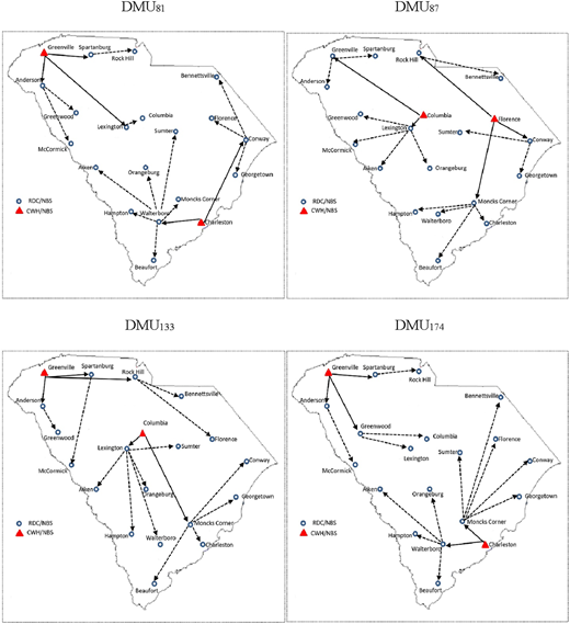
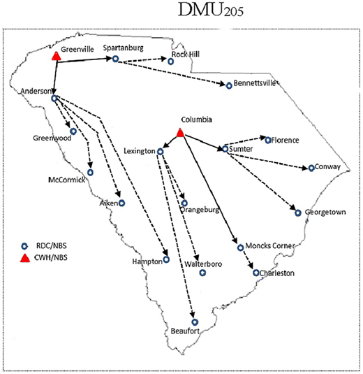
Tables 8–10 summarize changes in the top-five DMUs for each case generated by SSN- DEA and the transformed GTSN-DEA. As Table 10 shows, it is pretty evident that the rankings generated by GTSN-DEA do not change as significantly as the rankings generated by SSN-DEA. These results also support that the proposed GTSN-DEA method generates more robust rankings than the traditional SSN-DEA. The five top-ranked DMUs by any of the three methods are DMU₈₁, DMU₈₇, DMU₁₃₃, DMU₁₇₄ and DMU₂₀₅, which are depicted in Figure A1, where each DMU represents the humanitarian supply chain network (HSCN) configuration, including locations and allocations of ERFs.

Both DMU₈₁ by CES and DMU₁₇₄ ranked #1 by GTSN-DEA find {Greenville, Charleston} for the CWH locations. DMU₈₁ finds {Anderson, Columbia, Spartanburg} for RDCs covered by the CWH {Greenville} and identifies {Walterboro, Conway} for RDCs covered by the CWH {Charleston}. DMU₁₇₄ has the edge over DMU₈₁ regarding TLC (=TLC1 + TLC2), whereas DMU₈₁ has a greater CDE than DMU₁₇₄. In terms of MCD, DMU₁₇₄ is more efficient than DMU₈₁ except for the coverage distance from RDC {Moncks Corner} to NBS {Bennettsville}. The top-ranked DMU by SES, DMU₈₇, finds two CWH locations in the middle of South Carolina, {Columbia, Florence}. As mentioned before, DMU₈₇ has the highest CDE among all 26 efficient DMUs. DMU₁₃₃, ranked #1 by CES, finds two CWH locations, {Greenville, Columbia}, far from the coastal area and looks more balanced regarding MCD, ECD and CDE than the other three top-ranked DMUs by the SSN-DEA-based methods.

To investigate the effects of disruption risks, we perform a sensitivity analysis by changing the risk probability for the CWH location {Charleston} of DMU₈₁, which is the largest city in South Carolina and is regarded as the most susceptible to the weather among the five CWH candidate locations. If the risk probability for the location gets lower, the CWH location will not change. Thus, we gradually increase the risk probability, $q2$⁠, for {Charleston}, by 0.05 from the current probability of 0.250 and solve the WGP model with a weight set given to DMU₈₁. We check if the optimal CWH location is shifted from {Charleston} to a different location. The experiment results are summarized in Table A1, showing that the CWH location {Charleston} does not change until $q2$ rises from 0.250 up to 0.295. We observe that only the performance measures related to ECD, such as ECD0, ECD1 and ECD2, decrease as long as the CWH location is not changed. When we increase $q2$ from 0.295 to 0.300, the optimal CWH location is changed to {Columbia} with a higher risk probability of 0.375. Consequently, all the performance measures are also changed. Considering all five performance measures, the WGP model changes the optimal CWH location despite having a higher risk probability.

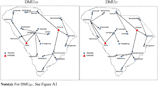
To see the effects of disruption risks more on the ERF location-allocation, we set all the probabilities of facility disruptions equal to zero, i.e. $pj=qi=0,∀jandi.$ Solving the WGP model for all 286 weight sets generates only eight (8) different configurations. See Table A2. Due to zero disruption probabilities, a significant performance measure, ECD would not differ among DMUs for the single-stage process. For the two-stage network process, there are only slight differences among DMUs for ECD0 and ECD1 at stage 1 and ECD2 at stage 2. We apply CE- and SE-DEA methods for the single-stage process and the GTSN-DEA for the transformed two-stage network process. Three methods identify three different top-ranked DMUs; DMU₈₇ by CE-DEA, DMU₁₀₁ by SE-DEA and DMU₂₇ by GTSN-DEA. Note that DMU₈₇, depicted in Figure A1, is selected as a top-ranked one by SE-DEA with disruption risks. From DMU₈₇ in Figure A1 and the other two top-DMUs, DMU₁₀₁ and DMU₂₇, depicting Figure A2, a significant effect of disruption risks is that all three top-rated DMUs have the common CWS location {Florence}. Note that the common CWS{Florence} has the highest disruption risk, and all three top-ranked DMUs choose the same RDCs {Rock Hill, Conway, Moncks Corner} for {Florence}.

The HSCN design has been a challenging problem whose goal is to relieve and minimize the effects of disasters and pandemics. For designing more balanced HSCN schemes consisting of ERF location and allocation, a WGP model is applied to generate various HSCN configurations. To evaluate these developed supply chain network schemes to identify the most efficient ones, the single-stage network (SSN) DEA models have been applied by various authors. The traditional C-DEA evaluates DMUs in terms of self-evaluation, allowing each DMU to rate its efficiency score with the most favorable weights. Consequently, problems related to weak discriminating power have arisen as the C-DEA is applied. The reason is that multiple DMUs frequently turn out to be efficient, so the lack of discrimination power is the major weakness of the C-DEA. Several methods based on the C-DEA model have emerged to remedy this weakness and increase discrimination. The cross-efficiency (CE) evaluation methods and super-efficiency (SE) models are typical techniques for ranking DMUs. Still, many studies reveal that these DEA models frequently do not generate consistent and robust rankings.

To overcome such shortcomings of SSN-DEA, this paper proposes transforming SSN into TSN so that GTSN-DEA is applied. The case study shows that the ranks generated by the single-stage process's CE- and SE-DEA models are not as consistent or robust as the GTSN-DEA. We observe that different HSCN configurations are ranked highly by the proposed approach, and these highly ranked schemes are ranked very low by the SSN-DEA method. In addition, the rankings produced by GTSN-DEA are not affected by the network schemes to be rated, while the ranks by the SSN-DEA models depend upon them under evaluation. Thus, the contribution of the proposed approach is to reveal the could-be hidden network schemes, if SSN-DEA is only applied, that the decision-makers would not consider as the candidate schemes for their final decision. This study demonstrates that the proposed GTSN-based approach would be an essential tool for designing these kinds of supply chain network schemes.

Environmental or natural disasters are one of the most challenging disruption risks that can cause one of the most potentially damaging. Particularly as the impact of global climate change continues to flow throughout the world, ERFs are frequently entirely disrupted, as shown throughout the world these days. Complete failure is the worst case of facility disruptions, so it would be interesting to consider the effects of partial failure of ERFs on the HSCN schemes and the ranks of efficient HSCN configurations as a future research direction. This paper considers the case of facility disruptions only. Future research will significantly enhance this study if the transportation disruptions, including route and transportation mode disruptions, are integrated with this study.

Several authors suggest future research directions for better performance of various supply chain systems. Fanoodi et al. (2019) apply artificial neural networks (ANNs) and auto-regressive integrated moving average (ARIMA) models to predict blood platelet demands with the aim of reducing the uncertainty in the supply chain. Goli and Malmir (2020) present an integer linear model for routing relief vehicles and using the covering tour approach, where the demand of damaged areas is considered as a fuzzy member, and fuzzy credit theory is used for optimization. With the emergence of distributed ledger technology (DLT), Roeck et al. (2020) provide the first empirical evidence of the impact of DLT on supply chain transactions, which will enable managers to improve their assessment of DLT usage in supply chains. Baziyad et al. (2022) provide an overview of the internet of Things (IoT) and investigate IoT applications and challenges in the context of supply chains. They (2022) identify four fundamental stages that should be considered in deploying IoT across a supply chain to support the digitalization of future supply chains. Khiabani et al. (2022) present a decision support system (DSS) based on neural networks and statistical process control charts for diagnosing and controlling myocardial infarction (MI) and continuously monitoring the patient's blood pressure. Their proposed method can help physicians make better decisions in diagnosing cardiovascular diseases. All of these proposed techniques, models and methods could be implemented to enhance the performance of the humanitarian supply chain systems.

ARD

Absolute Rank Difference

CDE

Covered Demand in case of Emergency

CDP

Commodity Distribution Point

CE

Cross Efficiency

CES

Cross Efficiency Score

CWH

Central Warehouse

DEA

Data Envelopment Analysis

C-DEA

Conventional DEA

CE-DEA

Cross Efficiency DEA

GTSN-DEA

General Two-Stage Network DEA

SE-DEA

Super Efficiency DEA

SSN-DEA

Single-Stage Network DEA

DMU

Decision-Making Unit

ES

Efficient Score

ECD

Expected Amount of Covered Demand

ERF

Emergency Response Facility

HSCN

Humanitarian Supply Chain Network

GP

Goal Programming

MCD

Maximum Coverage Distance

NBS

Neighborhood Site

RDC

Relief Distribution Center

SCRM

Supply Chain Risk Management

SES

Super Efficiency Score

TLC

Total Logistics Cost

WGP

Weighted Goal Programming