

This paper aims to design a vulnerability assessment model considering the multidimensional and systematic approach to disaster risk and vulnerability. This model serves to both risk mitigation and disaster preparedness phases of humanitarian logistics.
A survey of 27,218 households in Pueblo Rico and Dosquebradas was conducted to obtain information about disaster risk for landslides, floods and collapses. We adopted a cross entropy-based approach for the measure of disaster vulnerability (Kullback–Leibler divergence), and a maximum-entropy estimation for the reconstruction of risk a priori categorization (logistic regression). The capabilities approach of Sen supported theoretically our multidimensional assessment of disaster vulnerability.
Disaster vulnerability is shaped by economic, such as physical attributes of households, and health indicators, which are in specific morbidity indicators that seem to affect vulnerability outputs. Vulnerability is heterogeneous between communities/districts according to formal comparisons of Kullback–Leibler divergence. Nor social dimension, neither chronic illness indicators seem to shape vulnerability, at least for Pueblo Rico and Dosquebradas.
The results need a qualitative or case study validation at the community/district level.
We discuss how risk mitigation policies and disaster preparedness strategies can be driven by empirical results. For example, the type of stock to preposition can vary according to the disaster or the kind of alternative policies that can be formulated on the basis of the strong relationship between morbidity and disaster risk.
Entropy-based metrics are not widely used in humanitarian logistics literature, as well as empirical data-driven techniques.
1. Introduction
Global warming can increase the higher frequency of natural disasters such as floods and landslides. These, in turn, can cause substantial damage to local livelihoods and civilian infrastructure (Lim et al., 2017; Simpson, 2017; Torres and Pereira, 2017). In this paper, we show that some human actions can magnify the damage of such natural disasters. For example, settling in high-risk areas is a decision made under scarcity conditions. Public policy oriented to mitigate risks must consider this scarcity for the planning of disaster risk mitigation as this shapes the vulnerability of households to disasters.
Risk can be defined as the combination of vulnerability, hazard and exposure (Wisner et al., 2004; Twigg, 2004; United Nations Office for Disaster Risk Reduction, 2015). Vulnerability to disasters conforms the human part in the concept of risk: is defined as the foreseeable consequences of a damaging event on entities such as human lives, health, wealth or environment. The level of vulnerability to natural disasters is a concept that requires operationalization to be measured. A good indicator of vulnerability must consider features that can serve to differentiate the vulnerable unit from those nonvulnerable. In this regard, we argue that vulnerability to disasters has four dimensions: economic (Cutter, 2012; Folke, 2006; Adger, 2006; Eakin and Luers, 2006), health (Djalante et al., 2020) social (Schoon and Bartley, 2008; Cutter and Finch, 2008; Rapeli, 2017), and geographical (Mattea, 2019).
Economic and educational dimensions are important to recognize the vulnerability level and may shape the ability to reactivate the livelihoods after the disaster (Cutter, 2012; Folke, 2006; Adger, 2006; Eakin and Luers, 2006). During a disaster, health and morbidity can magnify the deprivation costs and affect the response and recovery (Djalante et al., 2020). Social capabilities are important for generating resilience by creating cooperation means within a community regarding the disaster response (Schoon and Bartley, 2008; Cutter and Finch, 2008; Rapeli, 2017). Geographical vulnerability depends on household location; those located in high-exposure districts are more likely to suffer from catastrophes Mattea (2019). Vulnerability is affected by all the possible interactions between those dimensions. We will show that all these features configure disaster vulnerability, defining it as multidimensional. We argue that households with an unstable economy, high morbidity regarding both chronic and acute illness, low social capabilities and geographical exposure to disasters are more prone to suffer from disasters, whether they happen or not. This selection of vulnerability dimensions is based on a welfare perspective, specifically in Sen's (1999) capabilities approach. In consequence, a limited set of capabilities in a household results in lower welfare and higher vulnerability. This is because fewer capabilities are traduced in fewer opportunities and this makes the disaster response and recovery tougher. This approach has the advantage that defines welfare in function of not only on economic status but also on educational, health, geographical and social status.
This paper reconstructs the classification of risky households made by the surveyors, in function of all the dimensions listed above that shape multidimensional vulnerability to disasters. Using logistic regression, we will give evidence that shows that vulnerability is a multidimensional problem. Risk is mitigated through the construction of resilience, which is equivalent to reducing vulnerability (UNDRR, 2017), and through preparedness policymaking. We will additionally make an experimental benchmarking to rank vulnerability at the province/district level. For this purpose, we will use entropy-based metrics to make systemic comparisons between communities/districts (Smyth and Hai, 2012; Yoon et al., 2017; Fatemi et al., 2020). Previous works have applied neither multidimensional nor entropy-based metrics for vulnerability assessment (Dong et al., 2016).
We implement the methodology in two Colombian communities: Pueblo Rico and Dosquebradas. We observe high heterogeneity between the cases: Pueblo Rico has a relatively small urban settlement, and the rest is composed of indigenous communities like Embera Chami or Embera Katio; in contrast, Dosquebradas has urban districts that are densely populated and a small rural zone. Both communities face risks of landslides, floods and housing collapse. The research questions are as follows: Which factors are key for mitigating disaster vulnerability for Pueblo Rico and Dosquebradas? With this information, what can humanitarian logisticians do to mitigate risks and improve disaster preparedness policies? The main contribution of this study is the use of informational entropy to support decision-makers in prioritizing public intervention in the risk mitigation and preparedness phases of humanitarian logistics, measuring the vulnerability of communities/districts. Following Alexander (2002), humanitarian logistics analyses four phases for the management of a disaster: the preparedness, the response, the recovery and the risk mitigation phases. This paper only covers risk mitigation and preparedness phases as there are few approaches in these (Overstreet et al., 2011; Leiras et al., 2014). For the former, the results can be useful for assessing vulnerability determinants. In this regard, the results contribute to the long-run planning of resilience in communities/districts. For the latter, a vulnerability assessment can lead to optimal locations for prepositioning stocks for humanitarian aid and determining the actions to be pursued according to the type of disaster; this is especially helpful in the short run. Furthermore, the demand for humanitarian aid is a direct function of vulnerability: the most vulnerable communities/districts will have higher demand and thus higher deprivation costs (Olorumtoba et al., 2018).
The remainder of this study is structured as follows. Section 2 presents the relevant literature and the theoretical framework. Section 3 describes the data collection procedures and the entropy-based methods to estimate disaster vulnerability. Section 4 outlines the main results and discusses them. Section 5 addresses the implications of our results for policymakers and stakeholders of the humanitarian supply chain. Finally, Section 6 presents the conclusions and recommendations for future research.
2. Theoretical framework
Here, we focus on the theoretical basis behind the estimation of the entropy-based vulnerability of households to disasters. The study of vulnerability is complex because it is a multidimensional and multi-causal phenomenon. Its evaluation requires processing a large number of variables that adequately characterize it. In this section, we present different concepts regarding entropy and entropy-based methods applied to urban, productive and humanitarian logistics that build an entropy-based vulnerability metric.
First, we briefly review the literature related to entropy, information theory and urban, production and humanitarian logistics. Second, we construct the theoretical framework based on previous works on multidimensional disaster vulnerability assessment. Third, we describe a community/district perspective for disaster vulnerability reduction.
2.1 A brief overview of the entropy method
In essence, entropy is said to be an expression of the disorder, the randomness of a system or the lack of information about it (Gray, 2011; Dong et al., 2016). Its measurement is useful for making decisions based on information about the entire system (captured in informational terms by the probability distribution). Considering households' disaster vulnerability, this variable can be defined as a system. This system is composed of interactions between different dimensions of disaster vulnerability. In this study, the entropy for households' disaster vulnerability is estimated from an entropy maximization problem which is restricted to information about the different dimensions affecting the system (Jaynes, 1957). When we want to compare two systems, we use cross-entropy methods (Krauz and Tabrikian, 2019; Ho and Wookey, 2020). Cross-entropy is a measure based on entropy and calculates the differences between two probability distributions, thereby estimating the distance between them. Specifically, we use the divergence of Kullback–Leibler (DKL) to analyze and compare probability distributions (Bouhlel and Dziri, 2019).
In the case of urban systems, Purvis et al. (2019) carried out a systematic literature review and observed that entropy is useful for measuring spatial concentration, dispersion of population growth and diversity of urban land use. In urban logistics, which represents an important part of urban systems, entropy is useful for multi-criteria decision analysis. Guoyi and Xiaohua (2011) evaluated two logistics providers based on multiple criteria, establishing entropy-based weights for each. Greater weight was assigned to those criteria where experts had a more uniform opinion, thereby valuing the consensus. In the field of production logistics, entropy has been used as an indicator of the complexity of the production process (Guoliang et al., 2017; Deng et al., 2017; Zhang and David, 2018). More complex processes imply higher entropy and lower efficiency for general operation.
2.2 A theoretical framework for measuring disaster vulnerability
Following Wisner et al. (2004) and Twigg (2004), we consider vulnerability as the human dimension of disasters and the result of the interaction of physical, economic, social and environmental factors. Disaster risk can be defined as the combination of vulnerability, danger and exposure and expressed as a probability of loss of life, injuries or destroyed or damaged assets (UNDRR, 2015). In the classic “Pressure and Release” (PAR) model (Twigg, 2004), vulnerability is declared as a progression: from root causes to dynamic pressures and ultimately to unsafe conditions. Then, disasters happen when unsafe conditions meet dangers. Table 1 shows the basic definitions that will be considered in this study:
Basic definitions regarding disaster risk
| Concept | Definition |
|---|---|
| Vulnerability | Is the foreseeable consequences of a damaging event on entities such as human lives, health, wealth or environment |
| Hazard | The loss of life or injury, property damage, social and economic disruption or environmental degradation caused by a potentially damaging physical event, phenomenon or human activity |
| Exposure | The property, people, systems or other elements present in hazard zones |
| Risk | The combination of vulnerability, hazard and exposure. We consider risk as an outcome of the vulnerability system. High risk is a result of high vulnerability, hazard and exposure |
Source(s): UNDRR (2015) and Twigg (2004)
Although the PAR model succeeds in explaining vulnerability progression, vulnerability metrics fail to capture information systemically. For example, Salazar-Briones et al. (2020) proposed an integrated urban flood vulnerability index composed of social, economic and physical factors. Furthermore, the vulnerability can also be affected by health or geographical factors (Eakin and Luers, 2006; Djalante et al., 2020). Even though a vulnerability index is comprehensive or multidimensional, it is calculated by normalizing each component and then averaging them up into one indicator. For example, Salazar–Briones et al.'s approach (2020) outputs a summary index of vulnerability. However, this index cannot provide information about the distribution of risk among the cities because it considers only the average between observations. The main disadvantage of this approach is that decision-making will not be based on the entire distribution but only on the mean values, thereby ignoring the information of extreme values. To formulate a systemic indicator that shows a measure of the system, we propose an entropy method approach. For this reason, the cross-entropy or the relative entropy (as measured by DKL) is the selected variable for entropy calculation. In this way, it is possible to assess vulnerability for each individual based on the characteristics of the group and the interrelationships of the different dimensions of vulnerability. Figure 1 presents the theoretical model that we use for estimating the vulnerability of households.
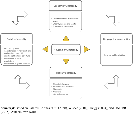
The selection of vulnerability dimensions is based on a welfare perspective: Sen's (1999) capabilities approach. From this perspective, vulnerability is associated with the set of capabilities of the population. The main idea behind this approach is that a limited set of capabilities in a household results in lower welfare and higher vulnerability. This is because fewer opportunities or capabilities can make disaster response and recovery tougher. This approach is multidimensional because it allows welfare to depend not only on economic status but also on educational, health, geographical and social status. Economic and educational dimensions are important to recognize the vulnerability level and may shape the ability to reactivate the livelihoods after the disaster (Cutter, 2012; Folke, 2006; Adger, 2006; Eakin and Luers, 2006). During a disaster, health and morbidity can magnify the deprivation costs and affect the response and recovery (Djalante et al., 2020). Thus, they are sources of vulnerability. Social capabilities are important for generating resilience by creating cooperation means within a community regarding the disaster response (Schoon and Bartley, 2008; Cutter and Finch, 2008; Rapeli, 2017). Geographical vulnerability depends on household location; those located in high-exposure districts are more likely to suffer from catastrophes. Thus, disasters can have significant spatial patterns (Mattea, 2019). All four dimensions mentioned above are very likely to be related to each other. The vulnerability may also be the result of all those possible interactions.
With this theoretical framework at the household level, we analyze the distribution of vulnerability metrics from a community/district perspective. Decision-making is better informed when we have tools for systemic diagnosis. Hence, we focus on the distribution of vulnerability within districts. Estimates for distribution are made with a statistical “rule of thumb” method: the kernel density estimation at the community/district level. This estimation is summarized via several graphs for community/districts to generate a systemic perspective of the entire distribution of vulnerability among households. Finally, we conduct student t-tests for significant differences between the vulnerability of districts (measured in terms of DKL).
The theoretical framework for household disaster vulnerability is applied for floods, landslides and collapses. One key assumption of this framework is that the vulnerability to those natural disasters has the same dynamics between units of analysis (Cutter, 2012; Folke, 2006; Adger, 2006; Eakin and Luers, 2006). Then, we can state the hypothesis formally:
There are similar vulnerability dynamics between disasters.
There are different vulnerability dynamics between disasters.
This hypothesis is theoretically supported by the relationship between welfare, capabilities and vulnerability to disasters. Our regression model tests the “similar vulnerability dynamics” hypothesis by determining the overall correlation of risk for different kinds of disasters for the entire sample.
2.3 Entropy theory as a tool for humanitarian logistics
The central aim of the humanitarian logistics discipline is to minimize the deprivation costs or the costs of suffering the lack of basic goods for disaster aftermath (Holguín-Veras et al., 2013). This is done by planning in four phases: risk mitigation, disaster preparedness, response and recovery (Overstreet et al., 2011; Leiras et al., 2014). To achieve this goal, the entropy-related literature has addressed the supply chain's diagnosis, the interaction between agents that compose a humanitarian response network and the performance of the institutions that provide support and supplies. Natural and anthropogenic disasters' damages are shaped by the level of vulnerability of the affected population. However, there is scarce literature that applies entropy as a framework to evaluate vulnerability regarding those disasters (Yoon et al., 2017). Humanitarian aid networks are special cases in which graph theory is used to study the flows between nodes and emulate a configuration based on the interaction of multiple actors involved in the humanitarian response (Comfort et al., 2009; Liyuan and Qingmei, 2014; Wu et al., 2013; Gomez, 2017). In network theory, entropy can be estimated from nodes, edges or topological measurements. At maximum entropy, the humanitarian response is disordered, every agent or institution is individualist, and there is a low density of cooperation (Wu et al., 2013). Comfort et al. (2009) determined that a network's entropy reaches its lowest value during a disaster and then increases over time. Therefore, it is necessary to focus on the preparedness phase to maintain a low entropy cooperation framework. Other metrics for measuring the performance of aid institutions are built based on the entropy theory, such as Theil's Index. It measures equity of the distribution of help and is especially useful when the minimization of deprivation costs alone is not sufficient to guarantee a low-inequity solution (Gutjahr and Fischer, 2018). The system is informing that maximum equity is reached at the maximum-entropy distribution of aid. Levner and Ptuskin (2015) also used the entropy method to identify vulnerability components within the supply chain related to disruptions, breaks, defects and errors. As is the case for humanitarian aid networks, risks are positively associated with entropy because it implies disorder in the humanitarian response. Entropy metrics depend on system attributes and complexity.
For the risk mitigation phase, the maximum entropy regression model allows the identification of those factors that are most related to disaster risk (Ben-Tal et al., 2011; Mateusz, 2017). Figure 2 shows how our procedure can contribute to risk mitigation.

A framework to estimate vulnerability from an a priori disaster risk classification
A framework to estimate vulnerability from an a priori disaster risk classification
When we run a regression, we can extract the vulnerability component from what disaster risk is by definition. Hazard and exposure analysis imply other types of predictive work, which involve disaster forecasts other than population and housing predictors (e.g. see Intrieri et al., 2019; Tshimanga et al., 2016). There is compelling evidence that development efforts address the root causes of vulnerability and can reinforce national, community and individual resistance and resilience to disasters (Goldschmidt and Kumar, 2016). For example, the building materials for households are classic vulnerability drivers. Their improvement is economically and temporally expensive. Furthermore, the multidimensionality of the study allows us to draw alternative policies from the results and propose more cost-effective (in terms of time and economic cost) interventions that contribute to risk mitigation. Based on our results, for the community/districts analyzed, a territorial framework for disaster vulnerability mitigation can be established, allowing for targeted risk mitigation (López-Vargas and Cárdenas-Aguirre, 2017).
Regarding disaster preparedness and humanitarian, Ukkusuri and Yushimito (2008) point out: “humanitarian logistics cannot be improvised at the time of the emergency since very little can be done after a disruption occurs”. A preferred disaster preparedness strategy is the prepositioning of inventory and supplies (Tofigui et al., 2016). Prepositioning enhances the postdisaster response because it has an important impact on the distribution cost (Ukkusuri and Yushimito, 2008). This prior positioning must be based on community/district vulnerability assessment, such as those resulting from the proposed model. Furthermore, the type of goods must match the type of disaster (Olorumtoba et al., 2018). Although the population density in rural areas is low and the location of aid points can be far and dispersed, vulnerability tends to be higher because of rural poverty. Therefore, these areas can be expensive to supply to as more vulnerability leads to more demand. The type of materials that are prepositioned depends on the type of disaster; this discussion is further extended in the “Managerial and research implications” section. Nevertheless, “far from cities” rural areas should not be an exception or receive less aid (Gutjhar and Fischer, 2018). In summary, the results of this model can be used to match the identified vulnerability patterns with the configuration of the humanitarian supply chain and the inventory prepositioning strategies.
3. Methodology
This section presents the methodology used for data processing and disaster vulnerability estimation at the household level. First, we explain the data gathering and processing methods. Second, we define the parameters and subscripts (see Table 2). Third, we explain the disaster vulnerability estimation methods in detail.
Categories retrieved by the dataset
| Dimension of vulnerability | Number of binary variables |
|---|---|
| Economic vulnerability | 41 |
| Social vulnerability | 17 |
| Health vulnerability | 23 |
| Geographical vulnerability | 24 |
| Total variables for MCA (all except geographical) | 81 |
Note(s): Without considering Geographical vulnerability binary variables, we have 81 variables
3.1 Data collection and description
The data were collected by the Risaralda Health Department considering the framework of the Collective Action Plan, called “Plan de Intervenciones Colectivas” - PIC (for its Spanish acronym), that is used to prioritize the neediest communities in the region. The sample was obtained in 2017 using a simple random sampling method. The sample size was determined as a function of the population size estimated using the census data of the Solidarity and Guarantee Fund (FOSYGA), a health insurance system aimed at the general population. The advantage of this database is its representativeness rate for nonurban inhabitants. This representation is higher than the XVIII Official Population Census and the VII Housing Census (2018).
The data collected contains economic, educational, health and social variables, following the framework presented in Figure 1. Along with the household head's education achievement, the household's physical environment (material and status, wealth, income and assets) was considered a part of its economic vulnerability. A social vulnerability was composed of the set of social abilities of the household members: the use of neighborhood structure, attendance in local associations and group activities. For health vulnerability, the following variables were considered: chronic diseases, morbidity, mortality, disability, nutrition and medical attention. Finally, for geographical vulnerability, we retrieved data for the district to which a household belongs. However, more sophisticated spatial patterns were not analyzed.
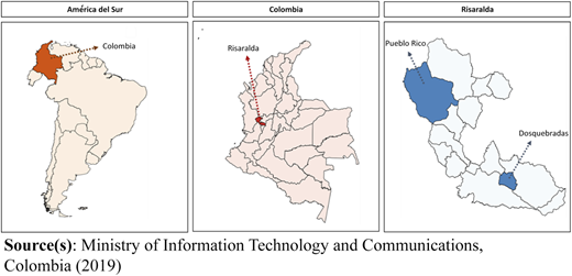
The impact of natural disasters in both municipalities is different. While there are more floods in Dosquebradas, there are at least three times more landslides and almost double the collapse of homes in Pueblo Rico. In terms of urban development, Dosquebradas presents an increase in the extent of the urbanized territory (density of 2532.5 “hab./km2”). In Pueblo Rico, there is only a small urbanized city next to other districts or unified shelters where the rural population is spatially dispersed to different degrees (density of 25.5 “hab./km”). Figure 3 shows the territory that Pueblo Rico and Dosquebradas occupy in Risaralda.
The Institute of Hydrology, Meteorology and Ambiental Studies (2019) reports rainfall with an annual variation of 2,500–9,000 mm and an average within 200–250 days of rainfall for Pueblo Rico and Dosquebradas. Although there is greater precipitation in Pueblo Rico (7,000–9,000 mm), there is less flooding risk reported in the survey. The more frequent landslides in Pueblo Rico can be explained mainly by the proximity between homes and mountains (an observation made in Google Earth Pro, 2019). Therefore, collapses are a more frequent phenomenon commonly caused by natural disasters because of the precarious construction of households.
The vulnerability dimension contains a high number of categorical and binary variables. Categorical variables were transformed into a set of additional binary variables to apply the multi correspondence analysis (MCA). Thus, Table 2 shows only binary variables. This approach was applied for reducing the dimensions of the original data set to a new set of linear indicators that can represent the maximum amount of data variances, such as in Filmer and Pitchet (2001), Ezzari and Verme (2012), Costa et al. (2013), Haregu et al. (2018), and Parchomenko et al. (2019).
3.2 An entropy-based model for disaster risk classification
3.2.1 Data processing methods
This section reviews the data processing methods. Table 2 shows a summary of the categories collected for each dimension of disaster vulnerability.
Geographical vulnerability variables are not considered in the MCA model because they cannot have multiple correspondences by definition: a household cannot be located in more than one place at a time. These variables are considered directly in the regression model as binary variables.
The MCA graph of the first two dimensions provides a graphic representation of the multiple correspondences between all the categories of the 81 binary variables. The MCA method can be summarized in three steps as follows.
First, the indicator matrix is recoded into a Burt matrix, where the indicator matrix is the original data set with the 81 binary variables defined as . The Burt matrix is defined as .
Second, we apply correspondence analysis in the Burt matrix (Rencher and Christensen, 2012). Then, we obtain the unadjusted principal inertias and the total inertia from a spectral or eigen decomposition of the Burt matrix. is the obtained eigenvalue. Then, is defined as the principal inertia for dimension , and total inertia is defined as .
Third, we predict the numeric output for dimensions as a linear function of the standard coordinates. Equation (1) shows this estimation for household . Then, is the matrix of standard coordinates, and is an element of the indicator matrix for the row and column . A similar formula was reported by Ezzari and Verme (2012) for their MCA application to multidimensional poverty.
where is the dimension score for household , and is the rows column vector of standard coordinates for dimension . Dimensions are linear functions of the standard coordinates, and they can be obtained by summing up every score and its respective category, divided by .
Finally, information about disaster risk is contained in three variables that take binary values: the value of these indicators is equal to one if the household has been positively classified as a risk of flooding, landslide or collapse; otherwise, they are equal to zero. These variables reflect both the incidence of natural disasters and the level of exposure to them. Most households located in areas with recurring disasters have a positive score on the risk indicator. We expect households located in such areas to have a positive risk indicator, even if they have a larger set of capabilities. These binary variables are considered as dependent variables in a regression model. This regression model is estimated following the maximum entropy theorem, instead of making assumptions about the distribution of the stochastic error terms or the behavior of the risk classification.
3.2.2 Vulnerability estimation methods
We propose three regression models for each of the three types of disasters in the sample: floods, landslides and collapses. For multinomial discrete choice models, we obtain the probability distribution that maximizes the entropy for the dependent variable. Soofi (1992) established a correspondence between maximum entropy logit and maximum likelihood logit, where the first-order conditions of the former are equivalent to those for the latter. Nevertheless, in small samples, the resulting coefficients will not be the same. Instead, the maximum entropy logit gives a family of logit distributions that are part of the generalized maximum entropy logit distribution (Golan et al., 1996). In the experiments carried out by Golan et al. (1996) for the theorems of Soofi (1992) using large samples (for example, N > 1,000), the generic logistic distribution is always the one that maximizes the entropy. Furthermore, this is also true for the maximum likelihood logit that outputs the same parametric results as the maximum entropy logit. In our case, the binary choice model is a special case in which we observe a binomial distribution for the dependent variable. Based on Soofi (1992) and Golan et al. (1996), we selected the logistic distribution for the estimation of the regression models to obtain a maximum entropy estimation of the distribution of probabilities among the sample.
Instead of estimating a model with a large number of binary variables, we reduced the dimension of the covariables by applying the MCA method. In this regard, the regression models account for a lower number of independent variables. The following regression equation (2) presents the model after the application of the MCA method application. We kept the first two dimensions after the MCA algorithm because they explain 72.6% of the total variance in the dataset.
The dependent variable of equation (2), , is the risk classification for the disaster for every household in the sample. The first variables, and , account for the first two dimensions from applying MCA. The geographic district location variables are then considered as independent regressors (housing location can be endogenous, but this issue is beyond the scope of this study) as well as the risk classification for the other types of disasters. A discussion of endogeneity regarding the risk classification for the other types of disaster is in Appendix 2. We proceed to an estimation considering and as endogenous regressors. While this is important for the robustness of inference, we show that this change does not have a significant impact on prediction.
The structural model considering endogenous regressors is as follows:
The selection of instruments was based on the assumptions of the two-step estimator for the logit model with endogenous regressors (Avery, 2005). First, , and then and . It is always better if there is a high correlation between instruments , and instrumented variables and . We test the assumptions and the exogeneity of the regressors.
The next step is to recover the vector of probabilities for risk classification. This is the distribution of the probability for a positive risk classification, which is estimated at the household level. It is important to have this information to generate tools that can provide insights based on the entire distribution, instead of a single metric summarizing the information for a territory. This distribution is later extracted for each territory in the sample. The following equation (3) presents the method used to estimate these probabilities:
These probabilities are estimated using the parameters obtained from the logistic regression (with endogenous regressors) for all households in the sample. The distribution of probabilities for the district (Equation 4) and the households (Equation 5) are as follows for every type of disaster :
At this point, we must note two distributions: the maximum-logistic probability distribution at the community/district level and the binomial probability distribution at the household level. With both distributions and , we can define the risk metric as a divergence from a low-vulnerability controlled scenario. This scenario is constructed with a simulated distribution for both and for each community/district. This algorithm is known as PageRank in several branches of data science literature (Sardhara and Lakhataria, 2019; Mo and Lee, 2019). Equation (6) shows the experimental setting:
where is normally distributed with a mean of and a standard deviation of , with the sub-sample sizes of , and . is the total sample size.
The next step is the cross-entropy calculus. We can alternatively estimate entropy for a community/district, but this estimation alone is difficult to compare between the districts without having a base scenario, which in this case is simulated as a low-vulnerability scenario as depicted above (Krauz and Tabrikian, 2019; Ho and Wookey, 2020). The following measure is known as the Kullback–Leibler divergence (DKL), which is used to capture systemic divergences between two different distributions of probabilities. This measure can be paired or unpaired. Here, we use the simplest version. Since we have a binary choice classification, it is measured in bits.
The two inputs for this measure are the two probability distributions, and . Divergence is obtained by summing across the binomial probability distribution , and thus, is estimated at the household level. The divergence is greater if and show very different patterns and information. For this case, is assigned to a low-vulnerability simulated distribution, which is used as a base scenario. Thus, a greater value of will show high vulnerability patterns (or high divergence from low-vulnerability scenario). This divergence metric captures systemic information and is constructed based on the multidimensional perspective of disaster vulnerability.
To build a community/district perspective for vulnerability, we output a graph of the kernel density for DKL metrics. We use the divergence from households within a community/district to generate a density of divergence from low-vulnerability scenarios. The following formula is computed for kernel density:
In equation (7), are weights for the sample. As the sample is random, those weights are all equal to 1. Then, and drive how many values are included in estimating the density at each point. We use a classical rule of thumb to estimate , which implies minimizing the mean integrated squared error (Silverman, 1986).
With the estimation at the household level, we conduct a set of student t-tests of means between the combinatory of 24 communities/districts that support the conclusions drawn from the graphics. The methodology for these tests is described in Appendix 4.
Figure 4 shows the step-by-step methodology and the value added of each step and estimation:
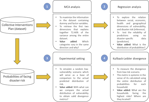
From step 1, MCA analysis, we can also condense all the information in the dataset into two variables, thereby simplifying the regression model and obtaining parsimonious estimates of vulnerability (defined by the probability of facing risks for landslides, floods or collapses). The experimental setting supports the postregression estimation of DKL. The more the divergence from a low-vulnerability scenario, the greater the household's vulnerability. With kernel densities of , we make both a graphic analysis and a nonparametric analysis with a student's t-test of means (results are shown in Appendix 4).
4. Vulnerability results and discussion
In this section, we present the results of the MCA. We simulated through MATLAB integrated software a basic scenario with a low probability of risk, a normal distribution with a mean value of 0.10 and a standard deviation of 0.01. This simulation was our comparison of the vulnerability distribution. We repeated the procedure for each community/district. Using the simulated and empirically estimated vectors of probabilities, we calculated . Finally, we plot the density of the DKL for the three cases: collapses, floods and landslides, to obtain a district perspective of vulnerability (non-parametric t-student tests of means are available in Appendix 4).
4.1 Multiple correspondence analysis
MCA provides continuous linear indicators and identifies associations between the original variables of our data set. Initially, the predictors contained many categorical variables. Therefore, the application of a regression model with a large number of categorical variables provides results that can be difficult to interpret, and there may also be multicollinearity between the variables. Thus, statistical inferences made about the covariables may not be reliable. Table 3 shows the MCA results.
Multiple correspondence analysis
| Dimension (Di) | Principal inertia | Proportion of variance | Cumulate percent |
|---|---|---|---|
| D1 (Wealth: assets, household status, access to services) | 0.0068 | 66.04 | 66.04 |
| D2 (Chronic diseases and related social support groups) | 0.0006 | 6.42 | 72.46 |
In Figure 5, the horizontal axis represents the number of dimensions retained, while the vertical axis shows the principal inertias. We observe that the first two dimensions make the form of an elbow. This method, called “the elbow method” is used for MCA and clustering models to determine the optimal number of dimensions (or clusters) to be retained. In the second dimension, the principal inertias show a significant decrease. We can argue that every additional dimension that we consider will have a negligible impact on the total variance explained, and instead, will lead us to a more complex interpretation of the data.
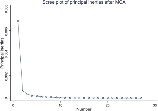
The size of our sample of households was 27,218, and the total inertia was 0.01. As noted before, we decided to keep the first two dimensions because both dimensions of the MCA analysis have a cumulative percentage of explained variance (which is equal to principal inertia divided by total inertia) that exceeds 72% of the original dataset. D1 had the highest proportion of variance value concerning the 81 binary variables, and D2 added information that captures the information for the remaining variables. The first dimension, D1, represents 66.04% of the variance ratio (according to the resulting principal inertias). This method allows maintaining the multidimensionality of the original data set while reducing its dimensionality. The dimensions were named following the obtained row scores for the standard coordinates ( in Equation 1). Figure 6 plots such standard coordinates in a graphic space. This MCA plot is a graphic representation of the multiple correspondences between 162 categories of the 81 analyzed binary variables.
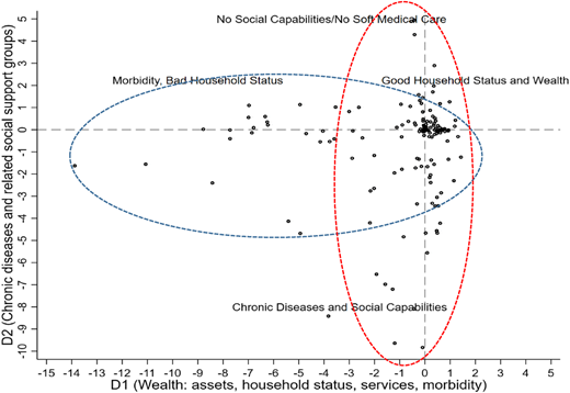
Figure 6 graphically shows the results from the MCA method. Each point represents a category (out of 162 categories) and is plotted as a function of its standard normalization scores. First, we found a cluster near the point where several categories have multiple correspondences. The blue circle represents all the categories associated with D1: negative values of D1 are related to high morbidity outcomes for households, while positive values are related to good household status and good practices of food cooking and waste management. The horizontal axis of Figure 7 presents categories ranked from highest to lowest by their scores. D1 takes values according to these scores. Also, fewer morbidity indicators in D1 mean better household status. These results suggest that this component is a representation of the economic and health dimensions of well-being. The small scores for social dimension variables show that there is a small association between D1 and social dimension. D1 is numerically constructed with economic, health and social variables. Thus, we decided to interpret D1 as “Multidimensional Wealth” (following Ezzari and Verme, 2012), which is also related to well-being in the sense of Sen (1999).
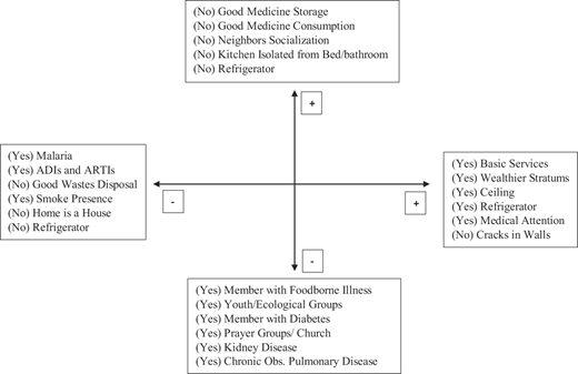
On the contrary, negative values of D2 are strongly related to chronic diseases that are less sensitive to changes in economic wealth or other variables affecting D1 (as shown in Figure 7). Some chronically ill people are more likely to belong to many kinds of social groups (the vertical axis of Figure 4 shows these relationships), while this characteristic also has a small incidence in D1 or multidimensional welfare. This aspect suggests that D1 alone fails to represent the multidimensionality proposed in the theoretical framework (economic, health and social vulnerability dimensions). We compensate for this issue by taking D2 as a complementary variable that not only captures chronicity aspects for health dimension but also captures social one which is associated with chronic illness. Thus, D1 and D2 together allow us to reduce the dimensionality of the original data set without losing multidimensional information for disaster vulnerability assessment.
4.2 Logistic maximum-entropy regression
In Table 4, we present the results of the margins of logistic regression evaluated at means for landslides, floods and collapses.
Maximum-entropy logistic results for risk classification
| Equation | (1) | (2) | (3) |
|---|---|---|---|
| Independent variables | Landslides | Floods | Collapses |
| D1 (endogenous) | −0.013*** | −0.004* | −0.014*** |
| (0.002) | (0.002) | (0.002) | |
| D2 (endogenous) | −0.000 | 0.000 | 0.001 |
| (0.001) | (0.001) | (0.001) | |
| Floods(a) | 0.096*** | 0.115*** | |
| (0.010) | (0.034) | ||
| Collapses(a) | 0.212*** | 0.097** | |
| (0.019) | (0.022) | ||
| Landslides(a) | 0.068*** | 0.186*** | |
| (0.013) | (0.017) | ||
| ROC | 0.86 | 0.88 | 0.85 |
| Accuracy (%) | 96.51% | 96.94% | 96.90% |
| Observations | 27,218 | 27,218 | 27,218 |
Note(s): Robust standard errors at the district level are in parentheses. We estimated them to evaluate whether there were heteroscedastic patterns between the districts. The geographic district variable's output was suppressed, but it is available in Appendix 3. P-values associated with t-tests for individual significance of coefficients: ***p < 0.01, **p < 0.05, *p < 0.1
The results of the model for each case – landslides, floods and collapses – had accuracies of 96.51%, 96.94% and 96.90%, respectively. The area below the ROC curve also suggested that a reliable level of fit was achieved, thereby allowing reliable predictions from those estimators. In terms of inference, the estimation of the model with endogenous regressors leads us to a robust significance of the effects. The model for landslides predicts that an increase in 1 unit of D1 (wealth, assets, access to education, housing material and status, access to services and morbidity) would cause a statistically significant decrease of 1.3% in the probability of facing landslides, maintaining all the other factors unchanged. The model for floods predicts a decrease of 0.4% in the probability of facing floods, given the same change in D1. This is not statistically significant, so it may be the opposite for some cases (confidence interval at 95% [−0.0088681, −0.0005697]). Finally, the model for collapses predicts a statistically significant decrease of 1.4% in the probability of facing collapses. The highest effect was for the collapses, which could be a completely foreseeable disaster.
For D2 (chronic diseases and related social support groups), the effects are not significant for all the sample sizes (it is possible to have significant effects on subsamples). A detailed endogeneity discussion for disaster risk classification is provided in Appendix 2. Our results are robust to the endogeneity of D1 and D2. The correlation matrix of the regressors in Table 4 is reported in Appendix 3.
Among the dimensions of the set of capabilities, the risk classification is largely explained by wealth: assets, household construction material, state of the home, access to services and morbidity contained in D1. Poor households are built with unstable material and are located in at-risk areas. On the contrary, neither the presence of chronic and infectious diseases nor does belonging to social groups of D2 has strong implications in the risk classification. This rejects the hypothesis constructed by Schoon and Bartley (2008), Cutter and Finch (2008), and Rapeli (2017). In relative terms, collapses are more sensitive to changes in D1 than other types of disasters. This may be explained by the fact that this type of disaster is strongly related to vulnerability. Consequently, to avoid housing collapses, it is necessary to improve the housing infrastructure, access to services and reduce morbidity. This is the same as in the case of landslides. Nevertheless, it is important to give differential treatment to floods. For Pueblo Rico and Dosquebradas, vulnerability to floods is not subject to economic, social, educational or health vulnerability.
Regarding D1 morbidity categories associated with lower wealth, education and poor practices of food cooking and waste disposal (see Figure 7), higher morbidity is associated with a high vulnerability for landslides and collapses. In this sense, the optimal policy should not focus only on the infrastructure but also consider morbidity to improve households' resilience (Djalante et al., 2020). An important result is that if a household is vulnerable to one type of disaster, it is very likely that it will be vulnerable to the other types. Thus, disasters are statistically related to each other. This result favors the “similar vulnerability dynamics” hypothesis for the three types of disasters, which means that landslides, floods and collapses may have similar vulnerability dynamics. Thus, we cannot reject H1 only based on our theoretical framework. Floods seem to be exogenous regarding the dimensions of disaster vulnerability. Therefore, variations in D1 and D2 may not affect the probability of facing floods.
Finally, the results for community/district control binary variables show that there are systematic differences in risk patterns between districts. Therefore, in the next section, we will discuss the results on divergence or level of vulnerability from a district perspective.
The strongest implication of these results is that disaster vulnerability is anthropogenic (at least for landslides and collapses). According to the theory, vulnerability is not only a result of interaction between humans and their physical context but also their economic and health aspects. However, disaster vulnerability does not seem to be strongly affected by differences in social capabilities or chronic illness, as seen in the results for D2. Consequently, a population with low human capital, low income, high morbidity and poor housing status tends to have greater disaster vulnerability regarding landslides and collapses. On average, people with these characteristics are those excluded from capitalist development, like indigenous communities. Morbidity is another vulnerability driver that comes with poverty, as suggested by the MCA results. Policies may have a quicker impact on morbidity than on poverty, considering that poverty reduction may be slower. Table 5 shows a legend for districts that is useful to understand the next subsection on vulnerability patterns from a district perspective.
Community/districts subsamples and nomenclature
| Nomenclature | Name | Definition |
|---|---|---|
| Pueblo Rico | ||
| KL1 | Urban Pueblo Rico | District |
| KL14 | Rural Pueblo Rico | District |
| KL15 | Embera Chami Zone 1 | Community |
| KL16 | Embera Chami Zone 2 | Community |
| KL17 | Embera Chami Zone 3 | Community |
| KL18 | Embera Chami Zone 4 | Community |
| KL19 | Embera Katio Zone 1 | Community |
| KL20 | Embera Katio Zone 1 | Community |
| KL21 | Santa Cecilia 2 | District |
| KL22 | Santa Cecilia 3 | District |
| KL24 | Villa Clareth 2 | District |
| Dosquebradas | ||
| KL2 | Commune 1 | District |
| KL3 | Commune 10 | District |
| KL4 | Commune 11 | District |
| KL5 | Commune 12 | District |
| KL6 | Commune 2 | District |
| KL7 | Commune 3 | District |
| KL8 | Commune 4 | District |
| KL9 | Commune 5 | District |
| KL10 | Commune 6 | District |
| KL11 | Commune 7 | District |
| KL12 | Commune 8 | District |
| KL13 | Commune 9 | District |
| KL23 | Rural Dosquebradas | District |
4.3 Disaster risk: a district perspective of vulnerability
4.3.1 Pueblo Rico households' distribution of divergence
DKL is always positive by definition. Our results for the three types of disasters and for all households in the sample are also positive. According to Table 6, the maximum divergence is 3.334. We observe smaller mean, median and variance indicators. Thus, we can state that disaster vulnerability is distributed around small values, with few atypical high-vulnerability cases. These divergence estimations also allow us to explore the vulnerability patterns between districts for each type of disaster.
Descriptive statistics from Kullback-Leibler divergence
| Disaster KLD | Mean | Median | Variance | Min | Max |
|---|---|---|---|---|---|
| Landslides | 0.117 | 0.091 | 0 .058 | 0.000 | 3.334 |
| Floods | 0.114 | 0.105 | 0 .033 | 0.000 | 3.163 |
| Collapses | 0.117 | 0.092 | 0 .052 | 0.000 | 3.291 |
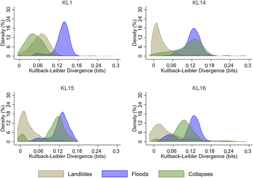
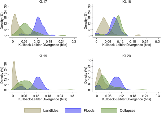
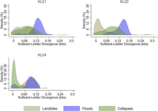
According to Figures 8–10, we observe an overall small divergence (0–0.3 bits) from the low vulnerability–simulated probability distributions for the three types of disasters. This evidence suggests that in Pueblo Rico province, households are more vulnerable to floods and collapses. The vulnerability to landslides is relatively small. Table 7 provides insights into the proportion of households with more than 0.3 bits of divergence in the sample.
The proportion of households with more than 0.3 bits of divergence in Pueblo Rico
| Community/District | Landslides | Floods | Collapses | |
|---|---|---|---|---|
| Pueblo Rico | ||||
| KL1 | Urban Pueblo Rico | 0.67 | 0.69 | 0.66 |
| KL14 | Rural Pueblo Rico | 0.20 | 0.22 | 0.22 |
| KL15 | Embera Chami Zone 1 | 0.18 | 0.18 | 0.18 |
| KL16 | Embera Chami Zone 2 | 0.17 | 0.18 | 0.18 |
| KL17 | Embera Chami Zone 3 | 0.12 | 0.12 | 0.11 |
| KL18 | Embera Chami Zone 4 | 0.10 | 0.11 | 0.11 |
| KL19 | Embera Katio Zone 1 | 0.21 | 0.23 | 0.20 |
| KL20 | Embera Katio Zone 2 | 0.11 | 0.12 | 0.11 |
| KL21 | Santa Cecilia 2 | 0.26 | 0.28 | 0.26 |
| KL22 | Santa Cecilia 3 | 0.17 | 0.19 | 0.17 |
| KL24 | Villa Clareth 2 | 0.05 | 0.05 | 0.04 |
Note(s): Values are in percentage
Representing indigenous communities, districts KL15-KL20 are less vulnerable to landslides but highly vulnerable to floods and collapses. Our evidence suggests that in Pueblo Rico, general disaster vulnerability is higher for floods and collapses. This may be explained by the geography of the territories. Along similar lines, there are relatively few “high vulnerability” cases within Pueblo Rico communities. However, almost every community has such cases, so it is reasonable to think that high vulnerability cases are spatially dispersed in Pueblo Rico.
Based on Figures 8–10, for the case of the districts KL1, KL14, KL22, and KL24, the pattern is the same as that for communities KL15-KL20: high vulnerability to floods and collapses. KL24 is an exception with lower vulnerability to collapses but high vulnerability to floods and landslides. It is important to conduct a deeper analysis of this district to explain these results. The “similar vulnerability dynamics” hypothesis does not seem to be true when we disaggregate the results to the communities/districts level. Thus, we can reject H1 in favor of H2 at this level.
It is important to note that we have higher divergence from low-vulnerability scenarios in Embera Chami Zone 2 (KL22) and Santa Cecilia 3 (KL16) for landslides (see Appendix 4: mean tests for evidence from formal statistical tests show the t-statistics to be positive and significant for the columns KL22 and KL16). These are cases with lower population densities, which face higher vulnerability than highly populated areas. The obtained results favor the hypothesis that low populated areas can face high risk (with higher vulnerabilities) as densely populated areas. However, rural risk mitigation can be challenging because of the cost of aid supply in terms of transport and the fact that higher vulnerability leads to greater demand requirements.
Stock prepositioning, as a strategy for disaster preparedness, in rural areas can be a way to cover the vulnerability gap in the short term. More stocks and materials in highly vulnerable districts can be located at strategic points where logisticians can start a delivery without losing materials. In the long run, humanitarian logisticians should also consider mitigating risks by reducing vulnerability via improving infrastructure, access to services, reducing morbidity and getting information about what risks can and cannot be mitigated, for example, floods that are exogenous to dimensions of vulnerability.
4.3.2 Dosquebradas households' distribution of divergence
For Dosquebradas, Table 8 gives us insights about the proportion of households with more than 0.3 bits of divergence in the sample:
Proportion of households with more than 0.3 bits of divergence in Dosquebradas
| Community/District | Landslides | Floods | Collapses | |
|---|---|---|---|---|
| Pueblo Rico | ||||
| KL2 | Commune 1 | 3.69 | 3.52 | 3.70 |
| KL3 | Commune 10 | 4.27 | 4.28 | 4.27 |
| KL4 | Commune 11 | 0.49 | 0.51 | 0.49 |
| KL5 | Commune 12 | 0.54 | 0.54 | 0.54 |
| KL6 | Commune 2 | 5.20 | 5.21 | 5.21 |
| KL7 | Commune 3 | 1.52 | 1.52 | 1.52 |
| KL8 | Commune 4 | 0.51 | 0.51 | 0.51 |
| KL9 | Commune 5 | 1.08 | 1.10 | 1.08 |
| KL10 | Commune 6 | 0.36 | 0.36 | 0.36 |
| KL11 | Commune 7 | 0.53 | 0.53 | 0.53 |
| KL12 | Commune 8 | 4.97 | 4.97 | 4.95 |
| KL13 | Commune 9 | 5.50 | 5.55 | 5.48 |
| KL23 | Rural Dosquebradas | 1.60 | 1.68 | 1.63 |
Note(s): Values are in percentage
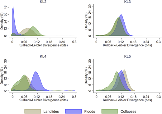
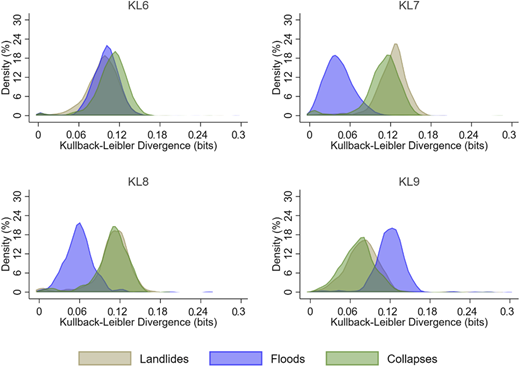
Based on Figures 11–13, we observed a lower vulnerability to landslides for KL3, KL6, KL10, KL11, KL12, and KL13. Relatively to Pueblo Rico's communities/districts, evidence suggests that vulnerability, regarding landslides, floods and collapses, is higher (see Appendix 4 for the mean tests). Landslides are more frequent in Dosquebradas. Some districts face minimum vulnerability to floods (KL2, KL7, and KL8), but a higher vulnerability to landslides and collapses.
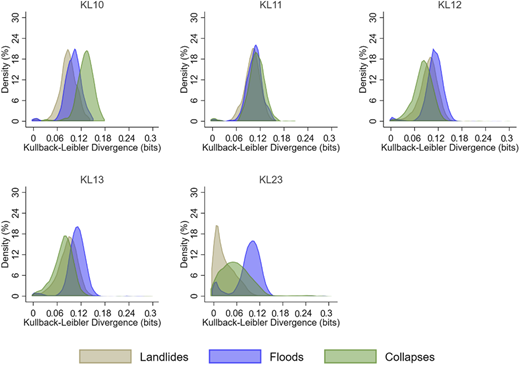
Density of Kullback–Leibler divergence for districts KL10, KL11, KL12, KL13 and KL23
Density of Kullback–Leibler divergence for districts KL10, KL11, KL12, KL13 and KL23
The low vulnerability districts (with an average of 0.1 bits of divergence from low vulnerability simulated scenarios) are KL10 and KL3. This can also be seen in the mean test in Appendix 4. The distribution of divergences suggests that Pueblo Rico had a slightly lower and more scattered (between households) level of vulnerability than Dosquebradas. While Pueblo Rico's vulnerability is higher for floods and collapses, Dosquebradas districts have similar vulnerability patterns for all three disasters (except for KL2, KL4, KL7, KL8, KL9, and KL23). Tables 7 and 8 show that there are more highly vulnerable atypical cases in Dosquebradas than in Pueblo Rico.
For both Pueblo Rico and Dosquebradas, although the risk mitigation recipes may be similar, the results (Figures 8–13) suggest that there is a need for specific materials according to the aftermath of disasters (Shao et al., 2020). Regarding floods, households may suffer from physical damage, but people's lives may be hardly exposed. This kind of disaster may not cause death, but it may cause significant losses in housing. For dealing with this aftermath, we recommend the prepositioning of food and beverage supplies and materials for shelters. We consider that epidemic-prevention drugs are important because of acute diarrheal disease and foodborne illness prevalence. In Appendix 1, we observe a greater prevalence in Pueblo Rico. For landslides, we have different aftermath. We expect a higher number of deaths. Therefore, we recommend prepositioning rescue materials and assigning rescue teams within the communities/districts. This is important if we want to reduce the risk of those disasters. Collapses could be a consequence of landslides or floods. However, they could also happen by other causes, like the poor housing condition. Following the proposed framework, material prepositioning may also help in dealing with collapses, even if they do not happen after another type of disaster. This is how we can approach resilience for Pueblo Rico and Dosquebradas.
5. Managerial and research implications
On the one hand, households' vulnerability estimation is important because decision-making can be made more informed on this basis. Furthermore, following this new approach, further academic research can propose alternative data-driven techniques to improve logistics operations. On the other hand, households' disaster risk can be defined as an open system in practice, that is, this risk's configuration may be affected by external forces. Thus, policies focused on reducing disaster risk vulnerability may indeed positively affect this system. We show that entropy is a useful tool to work with and summarize trends for multidimensional data. This work also generates evidence that shows that disaster vulnerability is multidimensional. Humanitarian logistics should consider this multidimensionality when planning for risk mitigation and preparedness.
Based on the graphic results and the student t-tests available in Appendix 4, we can establish a vulnerability ranking between the communities/districts in Pueblo Rico and Dosquebradas. The more vulnerable communities/districts are those that have the highest divergence. Table 9 presents this ranking:
Risk ranking of communities/districts in Pueblo Rico and Dosquebradas
| Order | Landslides | Floods | Collapses |
|---|---|---|---|
| 1 | KL23 | KL1 | KL23 |
| 2 | KL2 | KL22 | KL2 |
| 3 | KL4 | KL2 | KL8 |
| 4 | KL5 | KL23 | KL22 |
| 5 | KL7 | KL4 | KL7 |
| 6 | KL8 | KL9 | KL10 |
| 7 | KL22 | KL14 | KL4 |
| 8 | KL16 | KL15 | KL6 |
| 9 | KL13 | KL17 | KL11 |
| 10 | KL19 | KL21 | KL14 |
| 11 | KL3 | KL3 | KL19 |
| 12 | KL6 | KL13 | KL3 |
| 13 | KL11 | KL5 | KL13 |
| 14 | KL12 | KL12 | KL1 |
| 15 | KL21 | KL19 | KL5 |
| 16 | KL1 | KL11 | KL9 |
| 17 | KL9 | KL16 | KL12 |
| 18 | KL10 | KL6 | KL15 |
| 19 | KL14 | KL10 | KL16 |
| 20 | KL24 | KL8 | KL17 |
| 21 | KL15 | KL18 | KL18 |
| 22 | KL17 | KL20 | KL20 |
| 23 | KL18 | KL24 | KL21 |
| 24 | KL20 | KL7 | KL24 |
Note(s): Yellow highlighted cells belong to Dosquebradas and green highlighted cells, to Pueblo Rico
After disasters pass, risk mitigation policies aim to reduce the vulnerability to future disasters with a primary focus on restoration, returning life to normal and building back better (Goldschmidt and Kumar, 2016; UNDRR, 2017). We found two channels through which policymakers can reduce vulnerability to disasters. First, risk can be mitigated by reducing the vulnerability of households by improving infrastructure that can withstand landslides and collapses and investing in better household materials to strengthen resistance to collapses and landslides. For floods, we can only propose preparedness strategies based on our results and the context of our study (because the model predicted that is very unlikely that risk of floods can be mitigated by reductions in vulnerability). Along similar lines, we propose a constant refinement and effective inspection of building codes. If these do not exist, we recommend building it following UNDRR (2017) to create resilient buildings. Second, morbidity aspects of health have a strong effect on vulnerability to such disasters. Specifically, a higher incidence of acute respiratory infections (ARTIs), acute diarrheal disease (ADT) or malaria is strongly related to greater disaster vulnerability. Our recommendation is to consider patterns of morbidity as an alternative source of policymaking for disaster risk mitigation. Economic wealth and morbidity vary in the same direction for Pueblo Rico and Dosquebradas. Therefore, further research should focus on this relationship to mitigate risks through reductions in vulnerability associated with morbidity. Social capabilities and chronic illness indicators do not seem to be related to disaster risk reduction as their impact on vulnerability is not significant. Except for the two last indicators, the evidence here partially supports our main hypothesis: vulnerability is determined by a set of capabilities composed of economic, educational and health outcomes (Sen, 1999). Thus, a better or greater set of capabilities is important for disaster vulnerability and risk mitigation.
The number of households in a vulnerable situation is typically used as a criterion for location of aid. Thus, vulnerability can shape the decisions about where to preposition supplies. Supplying aid can be expensive if demand points are spatially dispersed (Gutjhar and Fischer, 2018). Location decisions about inventory prepositioning are important for reducing the cost of supplying to disperse rural areas with high vulnerability to disasters (Ukkusuri and Yushimito, 2008; Tofigui et al., 2016). In this regard, our results can serve disaster preparedness planning as demand can be estimated between and within communities/districts. Humanitarian logisticians can locate better, distribute inventory and stock before the disaster. Consequently, the cost of supplies is reduced if preparedness policies adopt inventory prepositioning based on estimated disaster vulnerability.
Prepositioning can also cover the high costs of supply to rural areas and indigenous communities (Ukkusuri and Yushimito, 2008). Thus, decision-makers should consider prepositioning materials to supply dispersed vulnerable areas far from the central warehouses. Furthermore, they should not preposition aid in vulnerable locations at risk of being impacted by the disaster (Goldschmidt and Kumar, 2016). The type of prepositioned supplies should consider the characteristics and consequences of the disaster. This has been a gap in humanitarian logistics research (Sabbaghtorkan et al., 2020). For example, in the case of landslides and collapses, the aftermath response must be fast using search, rescue and excavation equipment. In the case of floods, there are greater needs for shelters, food and health services to the population (de Brito Jr et al., 2020). More detailed evidence and routing problems are left for further investigation because there are few examples of routing in low densely populated rural areas (Huang et al., 2018).
The ranking in Table 9 serves as a policy tool. Humanitarian logisticians can pay more attention to highly vulnerable communities/districts. In both risk mitigation and disaster preparedness phases, the information about which households and which districts are more vulnerable can be used to improve the impact of humanitarian operations. By knowing what type of disaster will affect a community/district, the type of disaster vulnerability can be used for thorough public preparedness drills to increase emergency and management capacities. This strategy involves strengthening disaster preparedness for response, taking action in the anticipation of events and ensuring capacities are in place for effective response and recovery (UNDRR, 2017).
The methodology used in this study was extensive. To replicate the methodology, humanitarian logisticians should work with population and housing data available around the world in the format of household surveys. Disaster risk classification in household surveys is essential. Even if one has disaster risk classification alone for a set of households, one can use this information to replicate DKL and obtain a community/district ranking with a probabilistic approach. While we do work with multidimensional data, the vulnerability can be also estimated using a regression with socio-economic data or wealth and assets data. We argue that this can work because of the robust regression results for wealth predictors. This branch of literature can be further developed.
6. Conclusions and future research
In this work, we show that entropy theory and cross-entropy metrics can provide insights into the vulnerability dynamics of a closed system, like the households in Pueblo Rico and Dosquebradas. We evaluated the cross-entropy divergence using Kullback–Leibler divergence (DKL) metrics between our measured distribution and the one resulting from a simulated low-vulnerability scenario. These metrics show which households are more vulnerable to disasters using a systemic and multidimensional perspective. This aspect makes the metrics valuable for decision-making. However, the information considered in the disaster vulnerability model was the maximum possible, given that the database could retrieve only categorical variables. Nevertheless, the MCA method showed great capacity to process a large number of categorical variables and summarize them in two dimensions. These dimensions together explained 72.46% of the variance of the original database without losing the multidimensional perspective. Thus, the maximum-entropy logistic regression model can estimate the distribution of risk probabilities as a function of these dimensions at the household level.
We analyzed households from three types of communities/districts: urban, rural and rural indigenous communities. We found overall “similar vulnerability dynamics” for all the samples. However, when we tested this same hypothesis at the community/district level, different patterns for vulnerability were found. Thus, we can reject our hypothesis on similar vulnerability dynamics at more spatially disaggregated levels. This issue is due to the limitations of quantitative research methods, that is, the results obtained by these methods can be invalidated for specific subpopulations. Further qualitative or mixed research methods are needed to gain a deeper understanding of the disaster vulnerability dynamics within communities/districts. Similarly, the identified vulnerability patterns for each type of disaster can be used for communities'/districts' development and enhancing resilience against disasters. Furthermore, the multidimensional vulnerability perspective can provide insights on how to improve well-being and capabilities (Sen, 1999). Multidimensional vulnerability is transversal to adverse situations, like poverty and democratic representation, among others, which are not reduced due to disasters. Future research can investigate this aspect.
Following Wisner et al. (2004) and Twigg (2004), we consider vulnerability as the human part (or anthropogenic) of disaster risk. The dependent variables analyzed were risk classifications for landslides, floods and collapses. Therefore, we first tried to explain the three components of this risk classification: vulnerability, hazard and exposure. We observed that our data covered only the vulnerability part of the risk configuration. Nevertheless, vulnerability alone was a good predictor as we had good measures of model accuracy. However, the model is far from perfect. The obtained results from community/district analysis show that we need more sophisticated spatial data, like the georeferentiation of households, which can account for interactions with hazard and exposure. These aspects can be included in future variants of this model to improve its performance by fitting the data and generating entropy-based insights.
Finally, as proposed in the “Managerial and research implications” section, the results of these models can improve humanitarian operations, allowing data to drive the planning of risk mitigation and preparedness policies in humanitarian operations. The insights allow us to generalize the utility of population and housing surveys to measure the level of vulnerability to natural disasters. With these results, we can both mitigate risks in the long run and trace a preparedness strategy for the short run disaster risk mitigation. This methodology can be applied to any case of study, if the data on population, housing, health, social and geographical dimensions are available. We also argue that vulnerability metrics are a good proxy for the demand for aid, even if a disaster is not happening. We can use this information for risk mitigation and inventory prepositioning.
This research was supported by the Centro de Investigación de la Universidad del Pacifico (CIUP - Research Center of the Universidad del Pacifico) and the Coordination for the Improvement of Higher Education Personnel - Brazil (CAPES), Procad Defesa 88887.387760/2019-00.
References
Appendix
The Appendix files are available online for this article.
