


The purpose of this paper is to formulate and solve a new emergency evacuation planning problem. This problem addresses the needs of both able and disabled persons who are evacuated from multiple pick-up locations and transported using a heterogeneous fleet of vehicles.
The problem is formulated using a mixed integer linear programming model and solved using a heuristic algorithm. The authors analyze the selected heuristic with respect to key parameters and use it to address theoretical and practical case studies.
Evacuating people with disabilities has a significant impact on total evacuation time, due to increased loading/unloading times. Additionally, increasing the number of large capacity vehicles adapted to transport individuals with disabilities benefits total evacuation time.
The mathematical model is of high complexity and it is not possible to obtain exact solutions in reasonable computational times. The efficiency of the heuristic has not been analyzed with respect to optimality.
Solving the problem by a heuristic provides a fast solution, a requirement in emergency evacuation cases, especially when the state of the theater of the emergency changes dynamically. The parametric analysis of the heuristic provides valuable insights in improving an emergency evacuation system.
Efficient population evacuation studied in this work may save lives. This is especially critical for disabled evacuees, the evacuation of whom requires longer operational times.
The authors consider a population that comprises able and disabled individuals, the latter with varying degrees of disability. The authors also consider a heterogeneous fleet of vehicles, which perform multiple trips during the evacuation process.
1. Introduction
Over the past decade, there has been a growing interest in planning effective relief distribution networks. This is due to the increasing number of natural disasters occurring globally and their catastrophic impacts on human lives and on the global economy. Figure 1 presents a summary of natural disasters, as well as the people affected for the period 1990–2016 (EM-DAT (2017), www.emdat.be/). According to these data, the total number of reported disasters has slightly decreased during the last decade, and the number of affected people has increased, almost linearly. In particular, during the decade 2005–2014, disasters have affected 1.7bn people, resulted in 0.7m fatalities and caused damages of $1.4 trillion. Roughly 70 percent of fatalities were caused by natural disasters, such as earthquakes and tsunamis, and 30 percent by other types of disasters, including man-induced ones (www.unisdr.org).
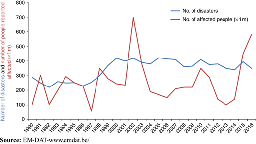
Total number of disasters and people reported affected (×1m) between 1900 and 2016 worldwide
Total number of disasters and people reported affected (×1m) between 1900 and 2016 worldwide
The dramatic effects of disasters have necessitated improved evacuation planning both during pre-disaster preparedness and post-disaster responsiveness. Evacuation plans define efficient procedures for evacuating individuals/households from areas at risk. Despite the fact that a part of the population would wish to use their private vehicles during the evacuation process, private car-based evacuation could lead to severe congestion, entrapment, increased injuries and/or unnecessary loss of life (Carpender et al., 2006). Thus, other forms of transportation such as organized public transport are needed and used (Liu and Yu, 2011).
This paper addresses organized and coordinated population evacuation by responsible agencies using available transport resources that have been identified a priori. The distinct features of the problem addressed are the following:
The population being evacuated includes both able individuals and people with mobility difficulties/disabilities. This is a very realistic and sensitive case, oftentimes not addressed thoroughly by either literature or practice. It is important to mention that according to the World Health Organization, about 15 percent of the world’s population has some form of disability, and 2–4 percent experience significant difficulties.
The available vehicle fleet is heterogeneous.
Vehicles are allowed to perform multiple trips in order to collect evacuees, and each pick-up location may be visited multiple times.
The plan addresses a transit dependent population and utilizes buses, as well as special vehicles for people with mobility limitations.
We define the related problem as the population evacuation using heterogeneous fleet problem (PEHFP), which concerns planning the evacuation of a population from pre-defined assembly points and transporting the evacuees to safe shelters. Appropriate authorities are responsible for the development of evacuation plans for areas with increased risk.
To define the problem with the required precision, we have developed a novel mixed integer linear programming (MILP) model. The latter seeks to determine the set of routes that minimize total evacuation time. Among the possibly multiple solutions that result to minimum evacuation time, the one with the minimum operational cost (or total travel time) is selected. The model includes multiple constraints that concern key operational aspects, such as routing, timing and vehicle/fleet capacity. We solve PEHFP by a new heuristic. We have selected the most efficient variant of the heuristic by solving a large series of sample problems. Subsequently, we analyzed the selected variant and applied it to a realistic case study.
The rest of this paper is organized as follows. In Section 2, we discuss the existing relevant literature and highlight the contribution of this paper. In Section 3, we describe the problem and define it precisely by developing a suitable mathematical formulation. Section 4 describes the two variations of the proposed heuristic algorithm and compares their efficiency. In Section 5, the selected, more efficient, heuristic is used to solve large-scale problems and performs sensitivity analysis. The proposed algorithm is applied to a case study in Section 6. Conclusions are discussed in Section 7.
2. Literature review
Several significant research works have focused on the emergency evacuation of populations. The main characteristics of such problems include the type of demand, the type of vehicles employed, the type of clients, as well as the methodology used to model the problem. The following paragraphs present significant papers categorized based on the characteristics described above.
Bish (2011) introduces a model for bus-based evacuation planning (BEP) along with two mathematical programming formulations, which are used to develop an effective heuristic algorithm. The objective in Bish (2011) is to transport evacuees from pick-up points to shelters in minimum time by using a fleet of capacitated and homogenous buses. The author analyzes the differences in the structural properties of optimal BEP solutions and those of the vehicle-routing problem. In Goerigk and Grün (2012), the authors introduce an extended version of BEP, called robust bus evacuation problem. In this case, vehicles are considered to be capacitated, they are allowed to make multiple trips, and the evacuees are transported to a single shelter. The demand is stochastic and a set of estimates for the demand is used for planning purposes. The decision about whether buses need to be dispatched immediately (based on the demand estimates) or to wait (until exact demand information is available) must be taken. Moreover, once a bus is routed its plan cannot be modified. The problem minimizes the maximum travel time of the bus fleet.
Perkins et al. (2001) consider the evacuation of a carless population in case of non-prior warning, placing emphasis on the case of a hurricane emergency. Buses perform a single trip and the problem formulation does not require the entire population to be evacuated. All buses are initially located at a depot, and the fleet is heterogeneous in terms of capacity. The aim is to find the optimal departure time of the buses from the depot in order to minimize the total travel time. In addition, travel times along network links are provided by a simulation model. The authors develop a binary integer programming model to derive a static optimal evacuation strategy.
In Margulis et al. (2006), a binary integer programming model is developed to address a simplified version of BEP. The objective is to maximize the number of evacuees within a certain time horizon for each bus, for each trip and for each pick-up location, taking into account capacity and availability constraints for both buses and shelters. Pick-up points are set according to the area’s zip code and the evacuees are assumed to access the nearest pick-up point. Additionally, the demand, i.e. the population inside this area, is estimated according to the official statistical data. It is also assumed that route travel times are known and constant for each bus and for each trip. Note also that each bus is allowed to carry out a maximum number of trips.
In Goerigk et al. (2013), the authors develop a “branch and bound” framework for the bus evacuation problem. The fleet of vehicles is capacitated and the demand is known. The buses are allowed to perform multiple trips, and the travel times are also considered known. In the work of Sayyady and Eksioglu (2010), the authors aim to maximize the number of evacuees with the resources available and minimize the total evacuation time. Each vehicle is assumed to perform only one trip and leave the pick-up location with full load. This assumption may lead to the case, in which a vehicle may not collect the entire population from a pick-up point due to the lack of capacity.
In Dikas and Minis (2016), the authors propose a two-index MILP to address the bus evacuation problem and its variants, and they develop a hybrid solution framework. The vehicles used are homogeneous, and the demand is known. Multiple shelters are used for the evacuees. The authors present extensive experimental results indicating that the proposed framework provides efficient solutions in reasonable computational times.
In Zheng (2014), an emergency evacuation strategy is presented, in which a homogeneous fleet of public buses serve a set of pick-up requests from pre-defined using a certain routing strategy and aiming to minimize the exposed casualty time. The delivery nodes in this case are of limited capacity and include both train stations and shelters. The demand is stochastic and the fleet of buses used is capacitated. The authors use a Lagrangian–relaxation solution approach and a simple example to validate the results obtained.
Recently, the work in Goerigk et al. (2014) introduces the integrated bus evacuation problem that extends the original model of Goerigk et al. (2013) by transporting passengers from their origins to multiple gathering centers. To address this problem, the authors developed a branch-and-price strategy and compared its efficiency using a commercial IP solver. In this case, the demand is considered to be known and the fleet of vehicles capacitated and homogeneous. Interested readers may also refer to Hamacher and Tjandra (2001), Altay and Green (2006), Bretschneider (2012) and Murray-Tuite and Wolshon (2013) for other research advances in the area of evacuation planning and emergency response.
It is also worth mentioning that the case of evacuation upon advance notice bears similarities with the vehicle-routing problem with satellite facilities. In such problems, vehicles are usually replenished at intermediate depots along their routes. Interested readers may refer to Murray-Tuite and Wolshon (2013) and Crevier et al. (2007) for further details. In the relevant literature, there are also other problems that reveal similarities with BEP, such as the multi-trip vehicle-routing problem. In such problems, vehicles are executing multiple trips in order to deliver or pick-up the total volume of products (Taillard et al., 1996; Brandao and Mercer, 1998; Petch and Salhi, 2003; Salhi and Petch, 2007). In the vehicle-routing problem with intermediate replenishment facilities, the aim is to determine optimal routes for a fleet of vehicles that can renew their capacity at intermediate replenishment stations (Tarantilis et al., 2008). Finally, the location routing problem (LPR) with capacity constraints applied to both depots and vehicles bears similarities with BEP. Belenguer et al. (2011), Prins et al. (2006) and He et al. (2009) solved the LPR and its variants using various techniques.
Table I overviews the relevant works of the existing literature discussed above, summarizing key characteristics of the problems addressed. From this table, it appears that the problems closer to PEHFP are those of Bish (2011), and Dikas and Minis (2016). Notable differences of the problems in Table I with PEHFP include the following:
In PEHFP, we consider the evacuation of different types of individuals, as characterized by their mobility requirements (e.g. able, partially and fully disabled). As discussed above, this is a very sensitive evacuation requirement.
In most related papers, vehicles are assumed to be of equal capacity; in PEHFP the vehicles are of different types and capacities (heterogeneous fleet).
In PEHFP each vehicle is allowed to make multiple trips in order to collect evacuees. In many related research papers each pick-up location is visited exactly once, while in PEHFP each pick-up location is visited at least once.
Taxonomy and categorization of evacuation and similar problems
| Demand | Type of fleet | Trip type | Travel times | Type of clients | Number of depots | Depot Capacity | Routes | Visits to Clients | Mathematical Model | Solutions | Solution approach | Case Study | |||||||||||
|---|---|---|---|---|---|---|---|---|---|---|---|---|---|---|---|---|---|---|---|---|---|---|---|
| Authors | A | B | C | D | E | F | G | H | I | J | K | L | M | N | O | P | Q | R | Exact | Heuristic | |||
Bish (2011) | X | X | X | X | X | X | X | X | X | MIP | X | Constructive Heuristic | No | ||||||||||
Gocrigk and Grün 2012 | X | X | X | X | X | X | X | X | X | MIP | X | Tabu search | No | ||||||||||
Perkins et al. (2001) | X | X | X | X | X | X | Not defined | X | X | BIP | X | Simulations | Yes | ||||||||||
Margulis et al. (2006) | X | X | X | X | X | X | X | X | X | BIP | X | Not defined | Yes | ||||||||||
Goerigk et al. (2013) | X | X | X | X | X | X | X | X | X | MILP | X | Branch and Bound | No | ||||||||||
Sayyady and Eksioglu (2010) | X | X | X | X | X | X | X | X | X | MILP | X | Tabu Search | Yes | ||||||||||
Dikas and Minis (2016) | X | X | X | X | X | X | X | X | X | MIP | X | Hybrid Solution Techniques | No | ||||||||||
Zheng (2014) | X | X | X | X | X | X | X | X | X | MIP | X | Lagrangian-relaxation | No | ||||||||||
Goerigk et al. (2014) | X | X | X | X | X | X | X | X | X | MILP | X | Branch-and-Price | No | ||||||||||
Bard et al. (1998) | X | X | X | X | X | X | X | X | X | MILP | X | Branch-and-Cut | No | ||||||||||
Brandao and Mercer (1998) | X | X | X | X | X | X | Not defined | X | X | Not defined | X | Tabu Search | No | ||||||||||
Petch and Salhi (2003) | X | X | X | X | X | X | X | X | Not defined | X | Constructive heuristic | No | |||||||||||
Salhi and Petch (2007) | X | X | X | X | X | X | Not defined | X | X | Not defined | X | Hybrid Genetic Algorithm | No | ||||||||||
Crevier et al. (2007) | X | X | X | X | X | X | X | X | X | MILP | X | Tabu Search | No | ||||||||||
Tarantilis et al. (2008) | X | X | X | X | X | X | X | X | X | Not defined | X | VNS, Tabu Search, GLS | No | ||||||||||
Belenguer et al. (2011) | X | X | X | X | X | X | X | X | X | BIP | X | Branch-and-Cut | No | ||||||||||
Escobar et al. (2013) | X | X | X | X | X | X | X | X | X | ILP | X | two-phase hybrid heuristic | No | ||||||||||
Prins et al. (2006) | X | X | X | X | X | X | X | X | X | BIP | X | Metaheuristic | No | ||||||||||
He et al. (2009) | X | X | X | X | X | X | X | X | X | Not defined | X | hybrid genetic algorithms, artificial neural network and hill climbing heuristic | Yes | ||||||||||
PEFHP | X | X | X | X | X | X | X | X | X | MILP | X | Heuristic | Yes | ||||||||||
Notes: A: deterministic, B: stochastic, C: homogeneous, D: heterogeneous, E: single, F: multiple, G: constant, H: dynamic, I: single, J: multiple, K: single, L: multiple, M: finite, N: infinite, O: constant, P: dynamic, Q: single, R: multiple, S: exact, T: heuristic | |||||||||||||||||||||||
All these critical characteristics of actual evacuation situations are captured by the proposed MILP model and are addressed by the proposed solution approach.
3. Mathematical formulation for the population evacuation using heterogeneous fleet problem (PEHFP)
3.1 PEFHP description
In PEHFP, a fleet of vehicles is required to pick up evacuees gathered at certain locations and transport them to safe locations (shelters). The population to be evacuated includes both able individuals and people with mobility problems. The latter are of two categories: people using wheelchairs that may be evacuated by vehicles equipped for that purpose, and people that may only be evacuated using an ambulance. The fleet of vehicles considered is heterogeneous, including vehicles of various capacities that may carry able passengers, accessible vehicles that may carry able as well as passengers with wheelchairs, and ambulances that carry passengers that require this service along, in some cases, with other types of passengers (in limited numbers of course). Consequently, PEHFP includes three different types of vehicles (of various capacities per type) and three different evacuee types. All vehicles start and finish their routes from/to different locations (depots). In the problem under consideration, the shelter is a single facility of unlimited capacity.
The problem objective is to determine the set of routes that minimize the total evacuation time; among the possibly multiple solutions with the minimum evacuation time, the one with the minimum operational cost (total time spent by all vehicle resources) is selected. Note that evacuation time is defined as the period that starts when the first vehicle(s) leaves (leave) the depot(s) to execute its (their) first trip(s) and finishes when the last evacuee arrives to a shelter. Furthermore, the total operation time is the sum of the operation times of all vehicles (till they return to the ending depots).
3.2 Mathematical formulation
Let C be the set of all nodes representing the evacuee locations, hereafter called pick-up nodes. Let Y be the set of evacuee types at each node, Y={a,w,s}, with a denoting the evacuees without any mobility problem (Type A), w denoting the evacuees using wheelchairs (Type W) and s the evacuees in need of stretchers (Type S). Additionally, let be the number of evacuees per type waiting at pick-up node i.
Let also {t} be the shelter of unlimited capacity (a single node) in which all evacuees will be transported to, and let be the set of available vehicles with Kj={1, …, uj} the available vehicles of type j={1, 2, 3}, where the three different types of vehicles are as follows:
Type j=1: these vehicles transport only evacuees without any mobility disabilities (able) and have a capacity .
Type j=2: these vehicles transport both able evacuees and evacuees using wheelchairs. Let be the capacity of vehicle k for able evacuees and be the capacity of the vehicle for evacuees using wheelchairs. Note that if a wheelchair position is not occupied by a disabled evacuee, then z able evacuees may occupy the freed space. Then, the total capacity of the vehicle in able only evacuees is .
Type j=3: ambulances which transport one evacuee on a stretcher, evacuees using wheelchairs (), and able accompanying person(s) ().
Since all vehicles start and finish their routes from/to different locations, we define two sets for the vehicle starting and ending locations, i.e., S={sk|k∈K} is the set of originating locations and E={ek|k∈K} is the set of the ending locations. Each of these locations may be considered as a single parking space. The locations are used to address the requirement of separating the total vehicle operation time from the evacuation time.
Let be an ordered set containing the possible trips of each vehicle k, assuming that , where is an indicator with if or 0 otherwise; this is the maximum number of trips required to pick up all evacuees by vehicle k. Let also be the set of all possible trips. Note that we will also use ancillary parameter to denote that the capacity per type of evacuee of trip v is equal to the capacity per type of evacuee of the corresponding vehicle making the trip.
We formalize now the definition of directed graph G(N, A), in which N={t}∪S∪E∪C is the set of nodes, A is the arc set connecting the nodes of N and is a set of triplets, with each triplet comprising an arc and a trip. Thus, let:
be triplets containing the arcs starting from the originating location of each vehicle k and the corresponding first trip. The first trip may be directed to a pick-up node, or to the ending location. The latter is used to model idle vehicles (if any).
be triplets containing: arcs connecting each pick-up node i∈C to all other pick-up nodes and to the shelter, and all trips except the last trip that is dedicated to the return of the vehicle to its ending location (from the shelter or from the originating location for possible idle vehicles).
be triplets containing arcs departing from the shelter and directed to all pick-up nodes by all trips except the first and the last one.
be triplets comprising arcs connecting the shelter with the ending location of each vehicle by its last trip.
Additionally, we define a set of pairs comprising trips arriving at certain nodes of the directed graph. Thus, we define the set , where:
contains only the first trip of each vehicle.
contains all trips, except the last trip of each vehicle that may arrive to the pick-up nodes and to the shelter.
, contains the last trip of each vehicle that arrives to the corresponding ending location. Note that an idle vehicle will be directed from the originating location to its ending location during its first trip, though a non-idle vehicle will make its last trip to its ending location.
Let be the minimum travel time between nodes i and j by trip v. Let also:
be the time that trip v arrives to node i.
be the number of evacuees of type y aboard the vehicle of trip v just before its arrival to node i.
be the number of evacuees of type y picked up from node i during trip v.
, , be the service time in node i during trip v, with tc and td denoting the time needed to collect or deliver a set of able persons and a single person with mobility disabilities, respectively. Note that independent of their number, the service time for a set of able evacuees is assumed to be tc.
be assigned the value 1 if arc (i,j)∈A is traversed by trip v, and 0 otherwise.
Tevac be the duration of the evacuation, i.e., the time span defined by the start of the evacuation until the time the last evacuee arrives to a shelter.
Then the objective function of the PEHFP is defined as follows:
where is the sum of the operation times of all vehicles and L ensures that the first term of (1) dominates lexicographically the second term: .
Optimization of (1) is subject to.
Routing constraints:
Timing constraints:
Capacity constraints:
Other constraints:
Regarding the routing constraints for all types of vehicles: Constraint (2) indicates that the first vehicle trip should depart from the originating depot. Constraint (3) ensures that all pick-up nodes should be visited at least once. Constraint (4) ensures that when one vehicle trip arrives at the shelter the next vehicle trip should depart from it. Constraint (5) indicates that trips of non-idle vehicles should arrive at the shelter, or idle vehicles should head directly to the ending location. Constraint (6) ensures that the first (for idle vehicles) or the last trip (for non-idle vehicles) should arrive at the ending depot. Constraint (7) ensures that if a vehicle arrives to a pick-up node it should also depart from this node within the same trip.
Regarding the timing constraints: Inequality (8) ensures that the evacuation time should be greater than the time of the last visit to the shelter. Constraint (9) defines the change of the arriving time at each node within the same trip. Constraint (10) defines the change of the arriving time for each next trip that departs from the shelter. Constraint (11) ensures that the time of arrival to any node will be greater or equal to 0, with B≫1, and, specifically, it will be equal to 0 if the node is not visited. Constraint (12) denotes that the first trip of each vehicle starts at time equal to 0.
Regarding the capacity constraints: Constraint (13) defines the change of the load for each trip, where B≫1. Constraint (14) ensures that every vehicle trip departs empty after a visit to the shelter; it also departs empty from its starting location. Inequality (15) ensures that at any node, other than the starting locations, the number of evacuees aboard a vehicle will not exceed the vehicle’s (trip) capacity nor it will be negative, and Constraint (16) denotes that each vehicle leaves the starting position and arrives at the ending position empty. For vehicles of Type 2 (k∈K2): Constraint (17) defines the change of the load on Type A evacuees for each trip, where B≫1. Inequality (18) ensures that at any node, other than a starting location, the number of able evacuees aboard a vehicle will not exceed the vehicle’s (trip) capacity for Type A evacuees nor it will be negative.
Regarding the rest of the constraints: Constraint (19) ensures that all evacuees should be picked up from all pick-up nodes by one or more vehicle trips. Finally, Constraint (20) defines the nature of the variable that denotes the number per type of evacuees picked up, and Constraint (21) defines the binary nature of the arc variables for each trip v.
The mathematical programming model of PEHFP assumes prior knowledge of the population to be picked up from each node, including able citizens and citizens with disabilities (of both types). Specifically, for each pick-up node problem inputs include the number of able evacuees, the number of evacuees using wheelchairs who will be transported by vehicles with certain technical characteristics and the number of evacuees who need to be transported by ambulances on stretchers. Note that for each node we assume that there will be a single pick-up point (assembly point) already been identified. This assumption does not present significant restrictions, since any probable intra-node distances and travel times for citizens that require home pick-ups are significantly shorter than the inter-node or the node to shelter distances and travel times.
Further input data include the exact node locations (pick-up nodes and shelter), and the corresponding road network connecting all nodes and the shelter. Note that the road network may offer the opportunity for more than one route to connect any two locations. Consequently, all network nodes and arcs should be provided, along with the corresponding distances and travel times.
Vehicle-related information includes the location of the starting point of each vehicle and the connecting road network, vehicle types and capacities per vehicle in terms of all types of evacuees.
4. Solution approach for PEHFP
The formulation of the MILP problem of Section 3 is of high computational complexity. As a consequence, problem instances of practical size may not be solved to optimality within reasonable computational times using exact methods, such as column generation with labeling algorithms (Dikas and Minis, 2016). Note that VRPs and other problems similar to PEHFP are NP hard resulting in exponential increase of complexity and solution times with problem size. For example, in Dikas and Minis (2016), one of the problems addressed is the BEP, which is very similar to PEHFP. The authors tested MILP exact solution methods for various problem instances and have concluded that larger-scale problems cannot be efficiently solved in reasonable time. In particular, the authors present results concerning the transportation of one or two evacuees per pick-up location collected from n=3, 4, 5, 6, 7, 8, 15 pick-up locations by two vehicles with capacity of three evacuees to two shelters. It is worth mentioning that for problems n=7 and 8, a time limit of 6 h was reached without obtaining the optimal solution, though for n=15 an optimal solution could not be obtained after 24 h. According to the results, the MILP for BEP cannot be solved to optimality for more than six pick-up locations even when one or two evacuees are waiting to be collected at each location.
For the above reasons, we propose a heuristic to solve PEHFP efficiently in reasonable computational time.
Prior to developing the heuristic for the full problem of Section 3, we test two alternative concepts in the simpler case that includes a single type of evacuees. In both concepts, the related algorithms plan efficient routes for the available vehicles in order to evacuate the population waiting at the pick-up nodes and transport the evacuees to the shelter. The routing plan evacuates the entire population, targeting minimization of the total evacuation time span, respecting the capacities of the available vehicles, the travel times between network nodes and all other constraints. The two alternative concepts are compared in terms of total evacuation time and the most efficient one is then applied to the more complex case that considers evacuees of different types of disability.
It is worth mentioning that disasters that evolve in an unpredictable manner, such as forest fires, may affect or damage transport infrastructure (e.g. road links), making some parts of the road network inaccessible. In such cases, alternative routes must be used. To deal with this complication, there is a need to update the available network, as well as the remaining demand and the remaining fleet, and resolve the problem. Under such circumstances the problem becomes dynamic (also see dynamic VRPs – in Psaraftis, 1988; Pillac et al., 2013) and may be addressed by re-planning and re-optimization (see also Ninikas and Minis, 2014).
4.1 The two alternative concepts
In the first concept C1, a list of vehicles (List) is arranged in descending order with respect to vehicle capacity. The first vehicle of List is routed to the node with the highest demand (always keeping a record of the corresponding travel time). If, after picking up the evacuees from this node there is remaining capacity, the vehicle is routed to its nearest node. The process is continued in the same manner until the vehicle’s capacity is exhausted or the total demand is met. The vehicle returns to the depot. If the routing process of the first vehicle is completed and the total demand is not satisfied, then the algorithm continues with the second vehicle of the List following the same process until the List is empty. In case List becomes empty and the demand is not satisfied, the algorithm identifies the vehicle that will return first to the shelter and continues performing the process described above until the total demand is met.
Note that although the vehicle routes are planned sequentially (one after the other), all available (or required) vehicles start executing their routes at the beginning of the operational time in parallel. Returning vehicles to the shelter are dispatched immediately as required by the plan.
In the second concept C2, the list of available vehicles (List) is again used. The routes of the vehicles in List are planned simultaneously. In particular, the first vehicle of List is routed to the node with the highest demand (always keeping a record of the corresponding traveling time), the second vehicle of List to the second node with the highest demand (again record traveling time), etc., until the List is exhausted or the demand of all pick-up nodes is met. If the List is exhausted and the demand is not met, the algorithm sorts the vehicles’ traveling times in ascending order and the vehicle with the minimum travel time is routed after it completes its first pick-up trip. If the vehicle with the minimum traveling time is at the shelter, it is routed to the node with the highest demand; otherwise it is routed to its nearest node. Routing of a vehicle en route continues till the vehicle’s capacity is exhausted or all demand has been served; upon either event the vehicle returns to the shelter. The algorithm continues in the same way till all evacuees have returned to the shelter.
The difference between C1 and C2 lies in the fact that algorithm C1 designs the routes sequentially while in C2 the routes are planned in parallel. However, for both algorithms the routes are executed in parallel.
The algorithms of both concepts were implemented in Matlab R2010b on a PC equipped with a 1.8 GHz Intel Core i5 and 4 GB of RAM. In order to evaluate the performance of the related algorithms, a set of sample evacuation problems has been generated and solved. Two sets of experiments have been conducted: in the first one, the number of pick-up nodes is fixed and the number of vehicles increases, while in the second set the number of nodes increases and the number of vehicles is fixed. For each vehicle-node combination, 100 problems have been generated and solved by both concepts/algorithms. Subsequently, the average evacuation time (AverageTevac1 for C1 and AverageTevac2 for C2, respectively) and the average total distance (AverageTotal_Dist1 for C1 and AverageTotal_Dist2 for C2, respectively) are computed for each algorithm per vehicle-node combination.
Experimental set 1: fixed number of operating vehicles
For each case corresponding to the number of nodes i=1, 2, …, 15 (i.e. 15 cases total) and v=5 vehicles, the generator creates 100 problems (15×100=1,500 problems in total). Both algorithms for C1 and C2 are used to solve each of these problems and determine the related evacuation plans along with the evacuation time and the total distance traveled by all vehicles. The corresponding average values are computed for each case i=1, 2, 3, …, 15.
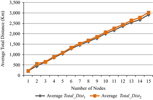
The results obtained are presented in Table II, and in Figures 2–5, respectively. In Figure 2, the average evacuation time for both algorithms is shown as a function of the number of nodes (and increases as expected). Similarly, in Figure 3, the average total distance covered by all operating vehicles during the evacuation problem increases with the number of nodes for both heuristics. Due to its nature, algorithm C2 utilizes more vehicles for meeting the demand (always respecting the maximum vehicle number). Thus, C2 performs better in terms of evacuation time, in comparison to algorithm C1, which is better in terms of the total covered distance.
Performance of algorithms C1 and C2 for v=5 vehicles and i nodes
| i | Average Tevac1 in min | Average Tevac2 in min | Average Total_Dist1 in km | Average Total_Dist2 in km | Percentage difference of Tevac (C1−C2) | Percentage difference of Total_Dist (C1−C2) |
|---|---|---|---|---|---|---|
| 1 | 151.7 | 151.7 | 215.4 | 215.47 | 0.00 | 0.00 |
| 2 | 211.5 | 184.6 | 439.8 | 557.68 | 12.70 | −26.79 |
| 3 | 235.8 | 221.1 | 636.9 | 652.62 | 6.24 | −2.45 |
| 4 | 322.7 | 294.4 | 852.2 | 894.5 | 8.77 | −4.95 |
| 5 | 365.4 | 333.5 | 1,037.4 | 1,090.1 | 8.73 | −5.08 |
| 6 | 425.1 | 399.7 | 1,289.5 | 1,335.7 | 5.98 | −3.57 |
| 7 | 476.2 | 442.5 | 1,460.2 | 1,525.5 | 7.07 | −4.47 |
| 8 | 511.7 | 478.6 | 1,625.5 | 1,681.4 | 6.47 | −3.43 |
| 9 | 564.2 | 523.9 | 1,782.0 | 1,852.5 | 7.15 | −3.95 |
| 10 | 624.3 | 587.2 | 1,999.4 | 2,075.2 | 5.93 | −3.78 |
| 11 | 665.4 | 631.3 | 2,166.7 | 2,260.5 | 5.12 | −4.32 |
| 12 | 718.6 | 669.6 | 2,366.1 | 2,445.6 | 6.81 | −3.36 |
| 13 | 769.2 | 720.2 | 2,545.3 | 2,644.1 | 6.35 | −3.88 |
| 14 | 804.5 | 753.9 | 2,674.2 | 2,781.6 | 6.28 | −4.01 |
| 15 | 855.9 | 814.2 | 2,917.2 | 3,020.9 | 4.86 | −3.55 |
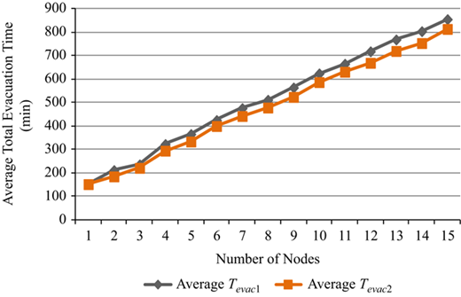
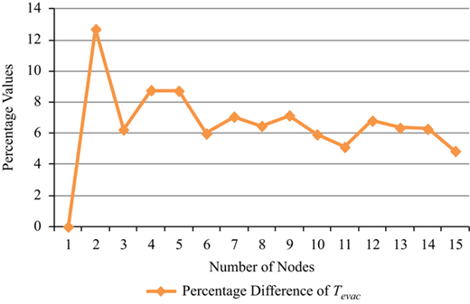
Percentage difference of average evacuation time for C1 vs C2 (v=5 vehicles and i=1, …, 15 nodes)
Percentage difference of average evacuation time for C1 vs C2 (v=5 vehicles and i=1, …, 15 nodes)
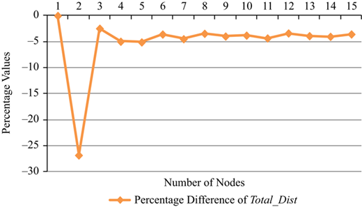
Percentage difference of average total distance for C1 vs C2 (v=5 vehicles and i=1, …, 15 nodes)
Percentage difference of average total distance for C1 vs C2 (v=5 vehicles and i=1, …, 15 nodes)
In Figure 4, the percentage difference for the average evacuation time between C1 and C2 is presented. It is clear that C2 performs better in all cases with i>1. As i increases, the percentage difference of the average evacuation time decreases. Note that in algorithm C1, in which routes are planned sequentially, a vehicle will not return to the shelter unless its capacity is met, or the total demand is met. Thus, in this case, a vehicle with remaining capacity seeks to determine the nearest pick-up node with non-zero demand in order to visit it and collect evacuees to meet its remaining capacity. Contrarily, in algorithm C2, in which routes are planned in parallel, a vehicle can return back to the shelter although its capacity is not met, because another vehicle route is scheduled for collecting the remaining demand in pick-up nodes. Thus, parallel routes in C2 manage to reduce the total evacuation time. However, as the number of nodes increases, the advantage of reducing the total evacuation time by parallel routes in C2 seems to be reducing.
Figure 5 presents the percentage difference of the average total distance. In this case, C1 outperforms C2. For i>2, the difference appears to be insensitive with respect to the number of nodes. Note that in C2 more routes are needed for collecting the evacuees and, consequently, the total distance is expected to increase.
Experimental set 2: fixed number of pick-up nodes
For each case corresponding to the number of vehicles v=1, 2, 3, …, 15 and i=5 nodes the generator creates 100 problems (15×100=1,500 problems in total). Both algorithms C1 and C2 are used to solve each of these problems and determine the related evacuation plans along with the evacuation time and the total distance traveled by all vehicles. The average values are computed and recorded for each heuristic and for v=1, 2, 3, …, 15.
Table III includes the results obtained. These results are also presented in Figures 6–9. In Figure 6, the average evacuation times for both algorithms are presented with respect to the number of vehicles used. As expected, the evacuation time reduces with the number of operating vehicles. Similarly, in Figure 7, the average total distance reduces with the number of vehicles for both heuristics C1 and C2.
Performance of heuristic algorithms C1 and C2 for 5 nodes and v vehicles
| v | Average Tevac1 in min | Average Tevac2 in min | Average Total_Dist1 in km | Average Total_Dist2 in km | Percentage difference of Tevac (C1−C2)(%) | Percentage difference of Total_Dist (C1−C2)(%) |
|---|---|---|---|---|---|---|
| 1 | 1,332.3 | 1,332.337 | 1,057.9 | 1,057.9 | 0.00 | 0.00 |
| 2 | 690.9 | 676.6 | 1,034.3 | 1,051.6 | 2.07 | −1.68 |
| 3 | 512.8 | 489.1 | 1,050.7 | 1,077.1 | 4.63 | −2.52 |
| 4 | 416.9 | 391.3 | 1,035.9 | 1,069.4 | 6.14 | −3.23 |
| 5 | 368.9 | 337.9 | 1,049.8 | 1,081.8 | 8.41 | −3.05 |
| 6 | 349.3 | 308.9 | 1,065.2 | 1,121.7 | 1,159 | −5.30 |
| 7 | 309.1 | 275.5 | 1,023.1 | 1,084.0 | 10.89 | −5.95 |
| 8 | 272.0 | 241.7 | 1,029.0 | 1,062.9 | 11.16 | −3.29 |
| 9 | 261.6 | 224.6 | 1,037.4 | 1,079.2 | 14.14 | −40.35 |
| 10 | 248.7 | 202.8 | 1,006.1 | 1,066.9 | 18.46 | −6.04 |
| 11 | 245.5 | 194.6 | 978.8 | 1,126.6 | 20.73 | −15.10 |
| 12 | 244.1 | 195.7 | 992.7 | 1,085.5 | 19.84 | −9.35 |
| 13 | 252.3 | 201.4 | 1,010.9 | 1,060.2 | 20.19 | −0.49 |
| 14 | 250.6 | 195.2 | 1,003.7 | 1,061.4 | 22.10 | −5.74 |
| 15 | 248.5 | 199.4 | 957.1 | 1,036.9 | 19.76 | −8.34 |
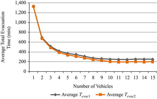
Average total evacuation time for C1 and C2 for v=1, …, 15 vehicles and i=5 nodes
Average total evacuation time for C1 and C2 for v=1, …, 15 vehicles and i=5 nodes
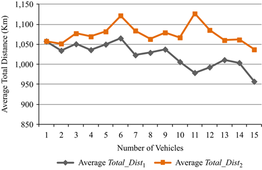
Percentage difference of average evacuation time for C1 vs C2 (v=1, …, 15 vehicles and i=5 nodes)
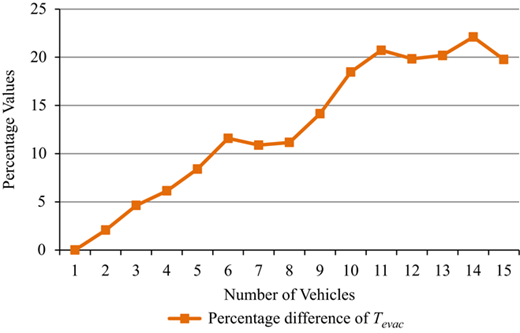
Percentage difference of average evacuation time for C1 vs C2 (v=1, …, 15 vehicles and i=5 nodes)
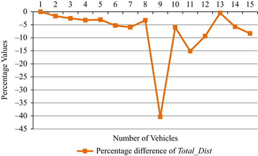
Percentage difference of average total distance for C1 vs C2 (v=1, …, 15 vehicles and i=5 nodes)
Percentage difference of average total distance for C1 vs C2 (v=1, …, 15 vehicles and i=5 nodes)
In Figure 8, the percentage difference for the average evacuation time between C1 and C2 is presented. C2 performs better in almost all cases. As mentioned above, algorithm C2 utilizes more vehicles for meeting the demand in comparison to algorithm in C1. Therefore, C2 manages to complete the evacuation process earlier than C1. As v increases the percentage difference of the average evacuation time increases.
Finally, in Figure 9, the corresponding percentage difference of the average total distance is provided. For all cases C1 outperforms C2 due to the fact that C2 tends to use more vehicles, when available, leading to an increase on the total distance covered. Note that the interesting difference in comparing the two algorithmic concepts comes from the fact that:
C2 results in faster evacuation times, while.
C1 results in shorter evacuation distance (traveled by all vehicles).
The objective we propose is evacuation time, and not distance as in most VRP problems (Golden et al., 2008; Toth and Vigo, 2014; Labadie and Prins, 2016). Consequently, C2 should be used in cases where the evacuation time is the objective to be minimized.
4.2 Proposed heuristic for a population that comprises able evacuees and evacuees with disabilities
Based on the results of Section 4.1, the second concept (C2), which performs better in terms of evacuation time, is used to address the full problem of Section 3. In this problem, we deal with able population and population with disabilities (Types A, W and S). As a consequence, vehicles with special characteristics are required for the evacuation operation. Evacuees of Type W need to be transported by vehicles that may carry wheelchairs (vehicles of Types 2 or 3), and evacuees of Type S can only be transferred by ambulances (vehicles of Type 3). Note that whenever a vehicle of Type 3 operates, it collects evacuees of Types W and A, as many as it can carry. Consequently, evacuees of Type A can be transferred by all types of vehicles. Additionally, a critical difference between the types of evacuees, concerns service time (loading/unloading). In particular, the service time depends on the evacuee type. Service time clearly affects the evacuation time.
In order to account for the fact that evacuees with disabilities (of both types) require higher service times, the proposed heuristic addresses the problem in two stages. The first stage deals with vehicles of Type 3 and evacuees with disabilities of Types S and W who use these vehicles, while the second stage deals with evacuees of Types A and W. This approach is introduced due to the characteristics of the vehicles as discussed at the beginning of Section 3.
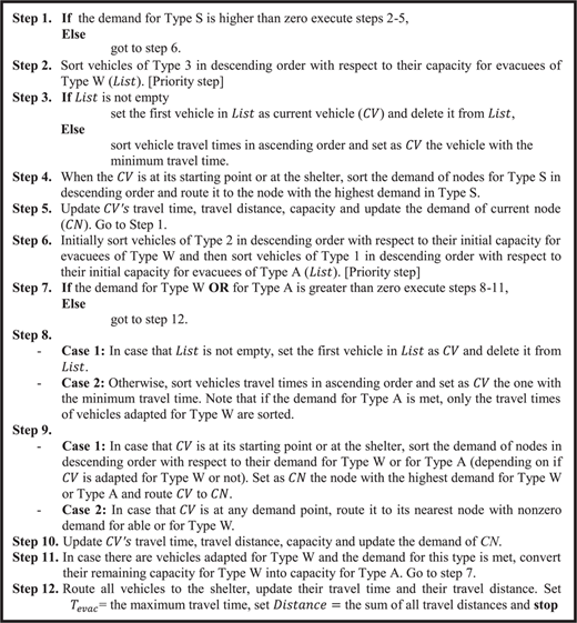
In the first stage, a list (List) of available vehicles of Type 3 (ambulances) is sorted in descending order of capacity for evacuees of Type W, since each vehicle may carry only one evacuee of Type S. Thereafter, the vehicles of Type 3 in List are routed simultaneously. In particular, the first vehicle of Type 3 in List is routed to the node with the highest demand for Type S (always keeping a record of the corresponding traveling time), it collects one evacuee of Type S and as many evacuees of Types W and A as it can transfer, if available. The second ambulance of List to the second node with the highest demand for Type S, etc., until the List is empty, or the demand of pick-up nodes for Type S is met. Note that in case there is more than one nodes with the same demand for evacuees of Type S, the vehicle is routed to the node with the highest demand for evacuees of Type W. Note also that in case the List is empty and the demand for Type S is not met, the algorithm sorts the traveling times in ascending order and the vehicle of Type 3 with the minimum traveling time is routed, after it completes its first trip, to the node with the highest demand for Type S. The entire process for the first stage is terminated when all evacuees of Type S are collected and sheltered.
In the second stage, a list of available vehicles (List) is initially created as follows: first the vehicles of Types 2 and 3 are sorted in a descending order with respect to their capacity for evacuees of Type W. This is because vehicles of these types can collect evacuees of both Types A and W, in contrast to vehicles of Type 1, and thus it is advantageous to route them first. Subsequently, the rest of the vehicles, which are not adapted for evacuees of Type W, are sorted in a descending order with respect to their capacity for evacuees of Type A. Thereafter, and at any point in the process, the first vehicle of List is routed; if the first vehicle in the List is capable to support evacuees of Type W, it is routed to the node with the highest demand for evacuees of Type W. Otherwise, if it cannot carry evacuees of this type, it is routed to the node with the highest demand for Type A evacuees. Always a record of the corresponding travel time, including the time need to collect all categories of evacuees at each visited pick-up node, is updated. The second vehicle of List is routed to the second node with the highest appropriate demand, and so on. This process is repeated until List is exhausted or the demand for both, evacuees of Types W and A, is met. In case that the List is empty, meaning that all vehicles are already sent for their first trip, and the demand is not met, the algorithm sorts vehicle travel times in ascending order and the vehicle with the minimum travel time is selected to be routed. In case the selected vehicle is at the shelter, which means that it has already completed a trip, it is routed to the node with the highest demand of evacuees of Type W or of Type A, depending on whether the vehicle may carry evacuees of Type W or not. However, if the selected vehicle is at any pick-up node, it may carry evacuees of Type W and the demand for this type is not met, then it is routed to its nearest node with non-zero demand for evacuees of Type W. In case the selected vehicle cannot serve Type W evacuees and it is currently at any demand node, then, it is routed to its nearest node with non-zero demand for Type A. The entire process for the second stage is terminated when all evacuees are collected from the demand points and they are sheltered.
It is worth mentioning that the proposed heuristic includes a proper prioritization for evacuees with disabilities (of Types S and W), which is necessary due to limited resources availability and due to the special treatment they need, as usually done in the humanitarian logistics literature. More specifically, the proposed heuristic plans first the routing of vehicles of Type 3 (ambulances) in order to evacuate disabled persons of Type W and S by sorting them in descending order with respect to their capacity for evacuees of Type W (note that all ambulances can collect only one evacuee of Type S). Thereafter, the algorithm plans the routes of Type 2 vehicles prioritized by their capacity to carry Type W evacuees. Only after the necessary, and available, routes of vehicles of Types 3 and 2 are planned, the routes of Type 1 vehicles are planned to evacuate able individuals.
Note that all vehicles, both the ones scheduled at the first algorithm stage and those scheduled at the second stage, start the route delivery simultaneously.
The steps of the proposed algorithm that addresses PEHFP for able and disabled evacuees are provided in Figure 10. The proposed process (see Steps 2 and 6, respectively) gives priority to evacuees of Type S, since the routes of the corresponding vehicles are planned first, and of Type W, since the list is formed by choosing the vehicles with W capacity first and sorting them in descending order. Furthermore, the process described in Figure 10 depicts the planning of vehicles’ routes. After the plan has been constructed, the vehicles to be used are dispatched simultaneously (i.e. in parallel). Thus, the use of the vehicles as well as the execution of the plan is performed in parallel.
The proposed algorithm needs to be provided with the necessary data in terms of the number and type of evacuees per demand node, the transportation network that links the demand nodes with the shelter, the transportation network between demand nodes, the transportation network that links each vehicle’s starting point with the demand nodes, and the fleet of evacuation vehicles per type.
As discussed above, the proposed approach for evacuation planning prioritizes evacuees based on their mobility abilities. However, it does not include any prioritization of locations (pick-up points). Such prioritization may be appropriate in case certain pick-up locations are imminently threatened. These locations may receive higher priority over others in the evacuation plan, that is, vehicles may be dispatched first to collect the related population. A two-step approach, i.e., solving the higher priority problem first, and the lower priority one subsequently, may be appropriate in such cases.
5. Analysis of the proposed approach
In order to demonstrate the applicability of the proposed approach of Section 4.2 to realistic cases, we present and solve a large-scale problem. Additionally, we perform an experimental analysis to investigate the effects of the problem parameters on evacuation time. The aim is to investigate whether the proposed approach is applicable to cases of realistic size and this issue is discussed in Sections 5.1 and 5.2, respectively.
5.1 Applying the proposed heuristic to a large-scale problem
To develop the large-scale problem, the following categories of data are required: evacuees and demand, network and available vehicles. More specifically the input data of the example comprise:
The total population per type of evacuee (A, W and S) and per pick-up node (see Table IV).
Vehicle starting and ending locations (12 vehicles in total in Table V), pick-up nodes (25 in total in Table IV) and shelter ({t}). The coordinates of these nodes have been generated randomly from the uniform distribution U (0 km, 20 km). To interpret our selection, note that we have arbitrarily considered that all abovementioned nodes can be placed in a circular area of 20-km radius.
The travel time as well as the traveling distance between all network nodes: distances have been calculated using the Euclidean form, and the average speed of all vehicles has been generated from the uniform distribution U (45 km/h, 55 km/h). This is an indicative speed for vehicles in populated areas.
For each available vehicle, the capacity per type of evacuee (see Table V).
The service time needed (for a vehicle of type 1 or 2) to collect/deliver any number of evacuees of type A is assumed to be 2 min; the service time needed (for vehicles type 2 or 3) to collect/deliver either an evacuee of type W or S is assumed to be 6 min per evacuee.
Population per type of evacuee for the pick-up locations (villages) for the large-scale example
| Demand | |||
|---|---|---|---|
| Pick-up nodes | Type A | Type W | Type S |
| C1 | 15 | 1 | 0 |
| C2 | 14 | 0 | 0 |
| C3 | 17 | 2 | 1 |
| C4 | 13 | 0 | 0 |
| C5 | 18 | 1 | 1 |
| C6 | 14 | 2 | 0 |
| C7 | 14 | 0 | 0 |
| C8 | 15 | 0 | 0 |
| C9 | 11 | 0 | 0 |
| C10 | 14 | 0 | 0 |
| C11 | 14 | 0 | 1 |
| C12 | 15 | 0 | 0 |
| C13 | 17 | 0 | 0 |
| C14 | 15 | 0 | 0 |
| C15 | 15 | 0 | 0 |
| C16 | 16 | 1 | 0 |
| C17 | 13 | 0 | 0 |
| C18 | 14 | 2 | 0 |
| C19 | 17 | 2 | 0 |
| C20 | 13 | 0 | 0 |
| C21 | 15 | 0 | 0 |
| C22 | 14 | 2 | 0 |
| C23 | 11 | 1 | 0 |
| C24 | 14 | 0 | 0 |
| C25 | 13 | 2 | 0 |
Available vehicles for the large-scale example
| Vehicle capacity | ||||||
|---|---|---|---|---|---|---|
| No. | Type of vehicle | Number of vehicles | Vehicle ID | Type A | Type W | Type S |
| 1 | 3 | 1 | 26 | 1 | 0 | 1 |
| 2 | 3 | 1 | 27 | 1 | 1 | 1 |
| 3 | 1 | 1 | 28 | 36 | 0 | 0 |
| 4 | 2 | 1 | 29 | 36 | 1 | 0 |
| 5 | 1 | 1 | 30 | 36 | 0 | 0 |
| 6 | 2 | 1 | 31 | 37 | 1 | 0 |
| 7 | 1 | 1 | 32 | 35 | 0 | 0 |
| 8 | 2 | 1 | 33 | 36 | 2 | 0 |
| 9 | 2 | 1 | 34 | 36 | 1 | 0 |
| 10 | 1 | 1 | 35 | 36 | 0 | 0 |
| 11 | 2 | 1 | 36 | 35 | 2 | 0 |
| 12 | 1 | 1 | 37 | 38 | 0 | 0 |
The results provided by the proposed algorithm for the evacuation of 25 gathering points and transportation of 361 evacuees of Type A, 16 evacuees of Type W and 3 evacuees of Type S to shelter {t} are provided in Table VI. The total evacuation time is 64 min, and the total distance is 238 km. All 12 available vehicles employed during evacuation. Note that the computational time is for this example is 1.09 sec.
Emergency evacuation plan for the large-scale example
| Number of transported evacuees | ||||||||
|---|---|---|---|---|---|---|---|---|
| Route No. | Type of vehicle | Vehicle ID | Node sequence | Starting time | Ending time | Type A | Type W | Type S |
| Routes operated by vehicles of Type 3 in the first stage | ||||||||
| 1 | 3 | 27 | *s27−3–{t} | 0 | 24 | 1 | 1 | 1 |
| 2 | 3 | 26 | s26−11–{t} | 0 | 13 | 1 | 0 | 1 |
| 3 | 3 | 26 | {t}−5–{t} | 13 | 25 | 1 | 0 | 1 |
| Routes operated by all vehicles in the second stage | ||||||||
| 1 | 2 | 33 | s33−19−14−{t} | 0 | 42 | [17, 4] | [2, 0] | 0 |
| 2 | 2 | 36 | s36−6−11−21−2−{t} | 0 | 34 | [14, 6, 7, 5] | [2, 0, 0, 0] | 0 |
| 3 | 2 | 31 | s31−18−9−4−2−{t} | 0 | 30 | [14, 6, 13, 4] | [1, 0, 0, 0] | 0 |
| 4 | 2 | 29 | s29−22−23−10−{t} | 0 | 30 | [14, 11, 11] | [1, 0, 0] | 0 |
| 5 | 2 | 34 | s34−25−12−21−{t} | 0 | 24 | [13, 15, 8] | [1, 0, 0] | 0 |
| 6 | 1 | 37 | s37−13−20−7−{t} | 0 | 23 | [17, 13, 8] | 0 | 0 |
| 7 | 1 | 28 | s28−5−24−2−{t} | 0 | 16 | [17, 14, 5] | 0 | 0 |
| 8 | 1 | 30 | s30−16−17−11−{t} | 0 | 21 | [16, 13, 7] | 0 | 0 |
| 9 | 1 | 35 | s35−3−1−9−{t} | 0 | 20 | [16, 15, 5] | 0 | 0 |
| 10 | 1 | 32 | s32−15−7−10−14−{t} | 0 | 33 | [15, 6, 3, 11] | 0 | 0 |
| 11 | 1 | 28 | {t}−8−{t} | 16 | 37 | 15 | 0 | 0 |
| 12 | 3 | 27 | {t}−5−{t} | 24 | 36 | 0 | 1 | 0 |
| 13 | 2 | 34 | {t}−25−{t} | 24 | 36 | 0 | 1 | 0 |
| 14 | 2 | 31 | {t}−22−{t} | 30 | 45 | 0 | 1 | 0 |
| 15 | 2 | 29 | {t}−23−{t} | 30 | 48 | 0 | 1 | 0 |
| 16 | 2 | 36 | {t}−18−{t} | 34 | 53 | 0 | 1 | 0 |
| 17 | 3 | 27 | {t}−3−{t} | 36 | 56 | 0 | 1 | 0 |
| 18 | 2 | 34 | {t}−1−{t} | 36 | 58 | 0 | 1 | 0 |
| 19 | 2 | 33 | {t}−16−{t} | 42 | 64 | 0 | 1 | 0 |
| Total evacuation time=64 min | Total distance=238 km | |||||||
Note: *si: originating location of vehicle with ID i
5.2 Experimental analysis
In this analysis, we examined the effects of the following parameters on total evacuation time:
service time per evacuee, for evacuee Types W and S; and
the number of available vehicles per type of vehicle.
To do so, for each set of parameter values we generated 50 problem instances. The characteristics of each instance are similar to the ones of the example presented in Section 5.1, with the following exceptions:
The vehicle capacities per type of evacuee (Types A, W, S) are shown in Table VII.
In total, 25 demand nodes are considered as follows:
the demand for evacuees of Type A at each demand point is generated from the Normal distribution N (15, 22);
the demand for evacuee Types W and S at each demand point is set to 0, 1 or 2 with probabilities 3/5, 1/5, and 1/5, respectively; and
at each demand point we assume that an evacuee with disabilities is of Type W with probability 9/10 and of Type S with probability 1/10.
Vehicle characteristics for the experimental analysis
| Capacity of vehicle per type of evacuees | ||||
|---|---|---|---|---|
| Type of vehicles | Number of vehicles | Type A | Type W | Type S |
| Type 1 | 5 | 30 | 0 | 0 |
| Type 2 | 5 | 20 | 3 | 0 |
| Type 3 | 5 | 1 | 1 | 1 |
Subsequently, for each set of parameter values we solved the corresponding 50 generated instances by adopting the heuristic of Section 4.2, and computed the average total evacuation time (one average value per each set of 50 instances). By varying the value of each of the above parameters, we were able to discern the effect of this parameter on the evacuation time.
In particular, consider the effect of service time for evacuees of Types W and S on total evacuation time. In this analysis, 15 vehicles are available (five per each type), and the service time varies from 3–8 min. The results are shown in Figure 11. As expected, the total evacuation time increases with service time. This increase is almost linear, indicating the direct correlation of these two variables.
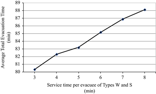
Effect of service time for evacuees of Types W and S on total evacuation time
Effect of service time for evacuees of Types W and S on total evacuation time
Consider now the effect of the number of vehicles per type on total evacuation time. In this case, we vary the number of vehicles from one to five for each vehicle type separately. In doing so, the other two vehicle Types remained at five vehicles each. Furthermore, the evacuation time for Type W or S individuals is 4 min. The results are shown in Figures 12 and 13, respectively. Figure 12 presents the (average) total evacuation time, whereas Figure 13 presents the percentage difference from the base case of five vehicles. As expected, by increasing the number of vehicles, the total evacuation time reduces in all three cases (vehicle Types 1, 2 and 3). The effect is more linear in the case of vehicle types that transport larger evacuee numbers and have higher capacity (i.e. vehicle Types 1 and 2). In the case of vehicle Type 3, the drop in total evacuation time is more severe, and it reaches a plateau. This is an interesting effect indicating that when increasing the number of vehicles beyond a threshold, the evacuation time is not affected. This threshold depends on the number of Type S evacuees.
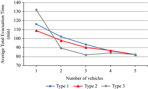
Effects of the number of vehicles (per type) on the total evacuation time (in min)
Effects of the number of vehicles (per type) on the total evacuation time (in min)
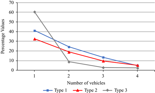
Percentage differences of total evacuation time from the initial case vs the number of vehicles
Percentage differences of total evacuation time from the initial case vs the number of vehicles
In order to further investigate the effect of number of available vehicles combined with service time (and thus any possible interaction), we conducted the following sets of experiments. For each value of the service time (3, 4, 5, 6, 7, 8 min), we have computed the (average) total evacuation time per number of available vehicles (1, 2, 3, 4, 5 vehicles). We did so for vehicle Types 2 and 3 (30 different cases per vehicle type – 60 cases in total). The results are shown in Figures 14 and 15, respectively. Figure 14 presents the variation of the average total evacuation time as a function of service time, per number of available vehicles of Type 2. Note that for the results of Figures 14, five vehicles each of Types 1 and 3 are considered. Figure 15 presents the same results for vehicles of Type 3. Note that vehicles of this type can transport both evacuees of Types W and S. Similarly to Figures 14, five vehicles each of Types 1 and 2 are considered.
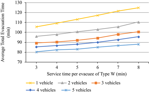
Effects of service time and available vehicles on the total evacuation time for vehicles of Type 2
Effects of service time and available vehicles on the total evacuation time for vehicles of Type 2
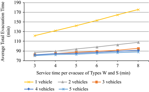
Effects of service time and available vehicles on the total evacuation time for vehicles of Type 3
Effects of service time and available vehicles on the total evacuation time for vehicles of Type 3
In both figures, the total evacuation time increases significantly with service time especially when fewer vehicles of each type are available. It is worth mentioning that Figure 15 validates the results obtained in Figures 12 and 13 for vehicles of Type 3; the evacuation time is not affected significantly by the increase of Type 3 vehicles beyond the threshold of three vehicles, indicating that it may not be advisable to include a larger number of such vehicles in the available fleet. However, this is not the case for Type 2 vehicles, the number of which clearly affects total evacuation time (for all values of service time).
The results of the above analysis reveal a clear dependence of the total evacuation time on the service time per evacuee of Types W and S and on the number of available vehicles of all types. To mitigate the effect of service time, the evacuation process designer could include more vehicles capable of transporting individuals with disabilities in the available fleet. Such a decision would improve evacuation time since more vehicles would operate in parallel collecting/delivering evacuees with disabilities. However, the designer should also take into account the threshold beyond which no considerable benefit is achieved (see Figures 12 and 13).
6. Case study
Further to the results presented in Section 5, a second goal is to investigate whether the proposed approach requires inputs that can be provided in practice and whether it can deliver results that may be used also in practice. These two issues are discussed below.
We have applied the proposed algorithm of Section 4.2 in the case of a forest fire in the Province of Teruel, Spain. This case study was conducted through an actual exercise that was performed in the field with physical presence of evacuees, pick-up points, a shelter facility, vehicles, other resources, a control center, etc. In order to simulate fire evolution in the exercise, specialized software was used supplied by the Government of Aragon. The forest fire initially threatens one of the three villages located in the area and the evacuation order was derived from the proposed algorithm. Subsequently, according to the simulation software, the fire evolves and threatens two other villages which should be evacuated. For this purpose, a new evacuation plan was designed, by re-using our algorithm. Based on information provided by the fire simulation software, the aim is to develop an appropriate population evacuation plan for the related province. In particular, we focus on obtaining good quality solutions for the evacuation of three small villages Tramacastiel (node B in Figure 16), El Campillo (node B in Figure 17) and Rubiales (node C in Figure 17), and the transportation of the evacuees to a safe shelter at the city of Teruel (node A in Figures 16 and 17). In the case study, the fire initially threatens Tramacastiel and its evacuation is ordered by the local authorities. Later the fire evolves and threatens both Rubiales and El Campillo. According to the simulation predictions, the fire approaches Rubiales and El Campillo a few hours later than Tramacastiel.
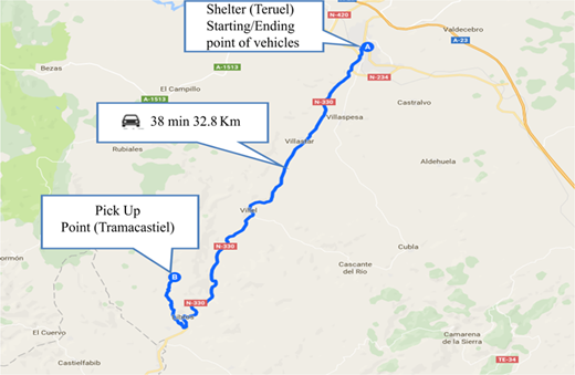
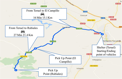
In order to apply the heuristic algorithm presented in Section 4.2 to the aforementioned evacuation case study, three categories of data need to be provided: evacuees and demand, network, and available vehicles as follows:
The total population per type of evacuee (A, W and S) for each village (see Table VIII).
Vehicle starting and ending locations, pick-up nodes and shelter.
The traveling time as well as the traveling distance between all network nodes.
For each available vehicle, the capacity per type of evacuee (see Table IX).
The service time for collecting/delivering evacuees of Type A is 2 min for all evacuees of this type, and the corresponding service time per evacuee of Types W and S is 6 min.
Population per type of evacuee for the pick-up locations (villages) at the Province of Teruel
| Demand | |||
|---|---|---|---|
| Village | Type A | Type W | Type S |
| Tramacastiel | 37 | 6 | 1 |
| Rubiales | 26 | 4 | 1 |
| El Campillo | 33 | 6 | 1 |
Available vehicles for the case study at the Province of Teruel
| Vehicle capacity | ||||||
|---|---|---|---|---|---|---|
| Vehicle | Type of vehicle | Number of vehicles | Vehicle ID | Type A | Type W | Type S |
| Car 4×4 | 1 | 1 | 5 | 4 | 0 | 0 |
| Van | 1 | 1 | 6 | 7 | 0 | 0 |
| Van | 1 | 1 | 7 | 8 | 0 | 0 |
| Van | 1 | 1 | 8 | 8 | 0 | 0 |
| Van | 1 | 1 | 9 | 8 | 0 | 0 |
| Patrol car | 1 | 1 | 10 | 4 | 0 | 0 |
| Patrol car | 1 | 1 | 11 | 4 | 0 | 0 |
| Patrol car | 1 | 1 | 12 | 4 | 0 | 0 |
| Patrol car 4×4 | 1 | 1 | 13 | 4 | 0 | 0 |
| Patrol car 4×4 | 1 | 1 | 14 | 4 | 0 | 0 |
| Common ambulance | 3 | 1 | 15 | 2 | 0 | 1 |
| Common ambulance | 3 | 18 | 16–33 | 2 | 0 | 1 |
| Common ambulance | 3 | 3 | 34–36 | 2 | 0 | 1 |
| Basic life support | 3 | 1 | 37 | 1 | 0 | 1 |
| Ambulance | 3 | 2 | 38–39 | 1 | 0 | 1 |
| Emergency mobile unit | 3 | 1 | 40 | 1 | 0 | 1 |
| Emergency mobile unit | 3 | 2 | 41–42 | 1 | 0 | 1 |
| Collective ambulance | 3 | 8 | 43–50 | 1 | 2 | 1 |
| Collective ambulance 4×4 | 3 | 2 | 51–52 | 1 | 1 | 1 |
| Bus | 1 | 2 | 53–54 | 55 | 0 | 0 |
| Bus | 1 | 1 | 55 | 22 | 0 | 0 |
| Bus | 1 | 8 | 56–63 | 50 | 0 | 0 |
| Bus | 1 | 2 | 64–65 | 55 | 0 | 0 |
| Bus | 1 | 2 | 65–67 | 22 | 0 | 0 |
| Bus | 1 | 4 | 68–71 | 55 | 0 | 0 |
| Small truck | 2 | 1 | 72 | 9 | 1 | 0 |
| Small truck 4×4 | 2 | 1 | 73 | 9 | 1 | 0 |
| Minibus | 2 | 1 | 74 | 22 | 3 | 0 |
All the aforementioned necessary input data are provided in Baou (2017).
The results provided by the proposed algorithm for the evacuation of Tramacastiel and transportation of the evacuees to Teruel are given in Table X. The total evacuation time is 112 min, and the total distance is 262.4 km; with four vehicles employed during evacuation.
Emergency evacuation plan: Tramacastiel to Teruel
| Number of transported evacuees | |||||||
|---|---|---|---|---|---|---|---|
| Route No. | Type of vehicle | Node sequence | Starting time | Ending time | Type A | Type W | Type S |
| Routes operated by Vehicles of Type 3 in the first stage | |||||||
| 1 | 3 | A – B – A | 0 | 112 | 1 | 2 | 1 |
| Routes operated by all vehicles in the second stage | |||||||
| 2 | 2 | A – B – A | 0 | 112 | 22 | 3 | 0 |
| 3 | 3 | A – B – A | 0 | 88 | 1 | 1 | 0 |
| 4 | 1 | A – B – A | 0 | 80 | 13 | 0 | 0 |
| Total evacuation time=112 min | Total distance=262.4 km | ||||||
According to the simulation scenario, the forest fire reaches Rubiales and El Campillo after the evacuation process of Tramacastiel is already completed. Consequently, the entire fleet of vehicles is available. Table XI presents the results provided by the proposed algorithm for the evacuation of Rubiales and El Campillo, while the corresponding routes are shown in Figure 17. The total evacuation time, after the evacuation of Tramacastiel, is 90 min, and the total distance is 249.2 km, with seven vehicles employed during the evacuation operation.
Emergency evacuation plan: Rubiales and El Campillo to Teruel
| Number of transported evacuees | |||||||
|---|---|---|---|---|---|---|---|
| Route No. | Type of vehicle | Node sequence | Starting time | Ending time | Type A | Type W | Type S |
| Routes operated by vehicles of Type 3 in the first stage | |||||||
| 1 | 3 | A – B – A | 0 | 68 | 1 | 2 | 1 |
| 2 | 3 | A – C – A | 0 | 90 | 1 | 2 | 1 |
| Routes operated by all vehicles in the second stage | |||||||
| 3 | 2 | A – B – A | 0 | 68 | 22 | 3 | 0 |
| 4 | 3 | A – C – A | 0 | 66 | 1 | 2 | 0 |
| 5 | 3 | A – B – A | 0 | 44 | 1 | 1 | 0 |
| 6 | 1 | A – C – A | 0 | 58 | 24 | 0 | 0 |
| 7 | 1 | A – B – A | 0 | 36 | 9 | 0 | 0 |
| Total evacuation time=90 min | Total distance=249.2 km | ||||||
From the results obtained, it is observed that collecting and delivering evacuees with disabilities, of both categories, has a great impact on the total evacuation time. This is reasonable since the service time during the pick-up and the drop-off process is significantly higher for an evacuee with mobility issues compared to an able evacuee. To deal with this fact, it would be beneficial to include more vehicles capable of transporting people with disabilities in the available fleet. Such a strategy would save valuable time resulting in faster and more efficient evacuation process.
Although of limited size, the value of the case study is that it was actually performed in the field encompassing all necessary requirements and practical details that are often ignored in theoretical studies. Thus the exercise included evacuees, both able and disabled, pick-up points at the locations presented above, a shelter facility, vehicles of various types, a control center that planned and monitored plan execution, and all other required resources (stretchers, wheel chairs), etc. The plan developed through the proposed approach was executed and all individuals were evacuated using this plan. Evacuation times were similar to the predicted ones. Furthermore, all inputs that are required by the proposed approach are practical, and in fact, readily available. Finally, the plan generated by the algorithm could be readily implemented and understood by all stakeholders. This validates the value of the proposed problem and approach.
7. Conclusions
In this paper, we presented the PEHFP. The latter deals with the evacuation of population comprising different types of evacuees: able, wheelchair users, individuals who need to be evacuated by an ambulance. To describe PEHFP precisely, a new mathematical programming model has been developed. The objective is to minimize the total time needed for evacuating the entire population from a set of pick-up points, respecting all related constraints. Comparing with the existing literature, the proposed PEHFP takes into account heterogeneous fleet, multiple trips, multiple visits at each pick-up node, and, importantly, treats different types of evacuees.
To solve PEHFP, we developed two alternative heuristic concepts. Extensive experimental study indicated that the algorithm which plans all available vehicles simultaneously is almost invariably superior in terms of total evacuation time as compared to the one the routes of which are planned sequentially. However, the latter is more efficient in terms of total distance traveled.
Based on the most efficient algorithm in terms of total evacuation time, we proposed an efficient heuristic for PEHFP. We tested its efficiency by constructing and solving a large-scale example. The solution provides a proposed evacuation plan in terms of vehicles used, routes to be run, total evacuation time and total distance. This plan was obtained in low computational time, validating that the proposed approach is practical for real-time evacuation planning.
The results of further extensive analysis indicated that there is a strong correlation between evacuation time and service time for individuals with disabilities. In addition, although the evacuation time decreases when more vehicles of all types participate in the evacuation process, a plateau in evacuation time is reached beyond which additional vehicles do not have a significant effect. This was observed in the case of low capacity vehicles that serve individuals with disabilities (i.e. ambulances), and should be considered in the emergency planning process. Using an appropriate number of larger capacity vehicles capable of evacuating people with mobility disabilities could lead to significant reduction in total evacuation time.
Finally, the proposed heuristic was applied to a case study, indicating its ability to provide efficient solutions for practical problems. The case study results also validated that evacuating individuals with disabilities has a great impact on total evacuation time, due to increased loading/unloading times.
This research has been co-financed by the European Commission (DG ECHO) under the MELOGIC project (ECHO/SUB/2014/695769). The authors would like to thank the rest of the project partners namely European University Cyprus (EUC), Caritas Diocesana de Teruel, HANKEN School of Economics, and Red Cross Italy (Vicenza Chapter), and especially Professor George Boustras, Professor Gyöngyi Kovács, Mr Pierandrea Turchetti, and Mr Jose Guillen. The authors would also like to thank the associate editor and the reviewers for their helpful and constructive comments that have helped considerably in improving the original paper.

