

This paper evaluates an alternative queuing concept for marine container terminals that utilize a truck appointment system (TAS). Instead of having all lanes providing service to trucks with appointments, this study considers the case where walk-in lanes are provided to serve those trucks with no appointments or trucks with appointments but arrived late due to traffic congestion.
To enable the analysis of the proposed alternative queuing strategy, the queuing system is shown mathematically to be stationary. Due to the complexity of the model, a discrete event simulation (DES) model is used to obtain the average waiting number of trucks per lane for both types of service lanes: TAS-lanes and walk-in lanes.
The numerical experiment results indicated that the considered queuing strategy is most beneficial when the utilization of the TAS lanes is expected to be much higher than that of the walk-in lanes.
The novelty of this study is that it examines the scenario where trucks with appointments switch to the walk-in lanes upon arrival if the TAS-lane server is occupied and the walk-in lane server is not occupied. This queuing strategy/policy could reduce the average waiting time of trucks at marine container terminals. Approximation equations are provided to assist practitioners calculate the average truck queue length and the average truck queuing time for this type of queuing system.
1. Introduction
To alleviate the recurring truck queuing problem at their entry gates, a growing number of terminal operators have utilized what is known as truck appointment system (TAS). In a typical TAS setup, trucks are required to complete their paperwork the day before their arrival to the terminal. This process expedites the processing of trucks' paperwork upon their arrival. Another benefit of the TAS is that it allows the terminal operators to put a limit on how many trucks can enter the terminal in a time-window (e.g. 2 h). Thus, the TAS provides a mechanism for the terminal operators to not only “smooth” out truck arrivals but also ensure that there are sufficient resources and capacity available to handle incoming demands. Many studies have evaluated the effectiveness of TAS (e.g. Zhao and Goodchild, 2013; Li et al., 2018), and many studies have developed optimization models to maximize the benefit of TAS for both terminal operators and drayage firms (e.g. Huynh, 2009; Huynh and Walton, 2011).
In current practice, the implementation of TAS is all or nothing. That is, if a terminal utilizes a TAS, it requires all trucks to make an appointment the day before their arrivals, and they need to arrive within their assigned time windows. Otherwise, they will be penalized a fee (Torkjazi et al., 2018). On the other hand, if a terminal does not utilize a TAS, then all trucks are allowed to arrive at their preferred times. For a terminal that utilizes a TAS, if a truck arrives late, it may make some of the trucks in the queue behind it miss their designated time windows. This study seeks to reduce truck queuing at terminals and ports by exploring a potential queuing strategy that allows late-arriving trucks and walk-in trucks to receive service via walk-in lanes to avoid affecting other trucks. The implication of this queuing strategy is that it does not abide by the first-in first-out principle. That is, there will be times when a late-arriving TAS truck receives service before those that arrived on time. This situation is similar to the system-optimal traffic assignment strategy where to achieve the lowest system travel time, it may be necessary to assign some travelers on routes with higher travel times than the user-equilibrium routes. That is, the system-optimal strategy is not fair to all travelers. It should be noted that the considered queuing strategy, one which allows switching, has not been implemented at any container terminal in the world, that is, it is a hypothetical concept. However, since it is a strategy that could reduce truck queuing time at the gate, it should be explored to provide terminal operators with additional means to lower truck turn time and increase gate throughput. The authors postulate that adding one or two such lanes could increase the effectiveness of TAS. Moreover, we do not believe having walk-in lane(s) will deter drayage operators from making appointments and use the TAS lanes because (1) service rate at TAS lanes will be higher than that of walk-in lane(s) and (2) the number of TAS lanes far exceed the number of walk-in lane(s). The proposed design is similar to toll booths in the US where there are several to many express lanes serving those motorists with E-ZPass and one or two lanes serving those motorists without the E-ZPass. Being able to traverse the toll booth without the need to stop is the reason why the majority of commuters opt to enroll in the E-ZPass system. We believe that rational drayage operators would apply the same logic to the proposed gate design and opt to make appointments and use the TAS lanes.
The objective of this paper is to explore an alternative queuing strategy for situations where there are two types of servers (TAS and walk-in) and arriving TAS trucks will switch from a TAS-lane to a walk-in lane if the TAS-lane server is occupied, and the walk-in lane server is not occupied. This queuing system is derived mathematically and is shown to be stationary. To assess its effectiveness, the average waiting number of trucks per lane is compared against the traditional single-class queuing model with no switching. Performance measures are obtained using a discrete-event simulation model due to the complexity of the queuing model. Additionally, simulation results are used to obtain approximation equations for calculating the average truck queue length and average truck queuing time. To our knowledge, this is the first study to investigate the scenario of a terminal serving both TAS and walk-in trucks and the first to propose a queuing strategy that allows TAS trucks to switch from a TAS lane to a walk-in lane.
2. Literature review
The following review focuses on related queuing studies; specifically, those which developed or utilized queuing models to analyze port operations and those used in other industries such as healthcare and airline where there are different user classes.
A number of studies have sought to analyze port operations by modeling each process as a queuing system. These processes include operations at the entry gate, container yard, and berth. At the berth, a well-known problem is the berth allocation problem (BAP), where the terminal operator assigns a berth to an arriving vessel with the objective of minimizing the vessel turnaround time. To determine the optimal vessel-to-berth assignment, researchers have treated the arrival and departure processes of vessels as a queuing system (e.g. Legato and Mazza, 2001; Roy et al., 2016). At the yard, researchers have formulated mathematical programs to optimize the use of the container yard that explicitly considered queuing processes of containers (e.g. Meštrović et al., 2018; Roy and de Koster, 2018). Since these types of models are intractable, researchers have resorted to using discrete event simulation (DES) models to solve them. Similarly, at the gate, researchers have developed mathematical models to determine the optimal appointment quota for a TAS by considering truck arrival and service process as a queuing system (e.g. Zhang et al., 2013; Chen et al., 2013).
Queuing theory has been applied extensively in other industries such as healthcare and airline. A complete review of queuing work in these areas is beyond the scope of this paper. Here, the studies which dealt with multi-server queuing systems in healthcare and airline industries are highlighted. Several studies have used multi-server priority queuing models to model patient flow in the emergency department (ED) (Masselink et al., 2012; He et al., 2012). Masselink et al. (2012) investigated the use of queuing models to quantify patient waiting time for medications at a pharmacy in a hospital. The authors proposed the use of a two-class GI/G/c queuing model to consider two different types of medication orders: priority and nonpriority. Almehdawe et al. (2016) developed a M[2]/M/2 nonpreemptive queuing model to capture two types of patient flow into an ED: one from ambulances and one from walk-ins. Badrinath et al. (2020) modeled the airport surface operations (i.e. runways and taxiways) as a multi-class M(t)/M(t)/q queuing model using operational data from three major US airports to reduce the waiting time, where the arrival/departure of the airplanes depend on its class.
To date, only a few studies have developed a queuing model that considers switching. In the work by Dester et al. (2017), the authors dealt with the join-the-shortest-queue (JSQ) policy often used for load-balancing purposes. They developed a simple analytical solution for the well-known problem with two parallel queues with finite capacity K, in which new customers join the shortest queue or one of the two with equal probability if their lengths are equal. In the work by Deng and Tan (2001), the authors studied a queuing system with a single server that switches service between two queues. Queue 1 is for nonpriority customers, and queue 2 is for priority customers. The switching policy is that the server would switch from queue 2 to queue 1 when the length of the latter reaches some level M. In their study, the authors derived the steady state joint probability generating function for the length of the two queues. Xie et al. (2008) dealt with multi-class priority M/M/s queuing model. When a server is available, the highest priority customer from the nonempty queue would switch to this server. Conditions for the queuing system to be stable/unstable were derived.
This study evaluates a new stationary two-class queuing model with two types of arriving trucks: TAS and walk-ins. In this proposed queuing model, TAS trucks are allowed to switch to walk-in service lanes if walk-in server(s) are idle. It is different from all previous work as follows: (1) all previously developed or applied queuing models in container terminal studies have only one class and (2) the majority of multi-class queuing models that have been applied in other industries do not have switching policy. A few queuing studies have considered switching. This paper is different from those as follows: (1) unlike the classic JSQ model, this study considers two different types of trucks and two different types of service lanes, and (2) unlike previous work that considered switching, in this study it is the trucks (not the servers) that have the option to switch to a different service lane.
3. Problem statement
Figure 1 illustrates the proposed two-class queuing strategy with switching; the term two-class refers to the two types of trucks and corresponding services. As shown, most lanes will be dedicated to serving trucks with appointments (referred to as TAS lanes), with one or two lanes reserved for walk-in trucks (referred to as walk-in lanes). The TAS lanes are dedicated to serving trucks with appointments arriving on time, and the walk-in lanes are dedicated to serving walk-in trucks or trucks with appointments arriving late. The switching policy is such that trucks with appointments, upon arrival, will switch to a walk-in lane if all TAS lanes have queues and all TAS-lane servers are occupied, and the walk-in lane is empty, and its server is not occupied.
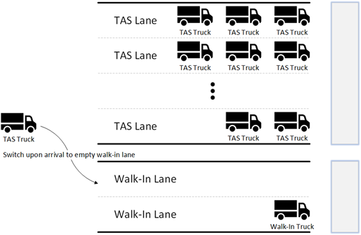
The queuing system addressed in this study considers two types of trucks: (1) with appointments arriving on time (TAS trucks) and (2) without appointments or with appointments but arriving late (walk-in trucks). Both TAS trucks' and walk-in trucks' arrivals are assumed to be independent of one another and are assumed to have different average arrival rates, and , respectively. There are two types of service lanes, TAS lanes and walk-in lanes, both with infinite queuing capacity. TAS lanes are reserved for TAS trucks, and walk-in lanes are reserved for walk-in trucks. However, TAS trucks upon arrival will switch to a walk-in lane if all the TAS lanes have queues and all TAS-lane servers are occupied, and the walk-in lane queue is empty, and its server is not occupied. Both TAS trucks and walk-in trucks are assumed to have different average service rates and , respectively. In addition, to avoid the infinite queues for this system, one restriction should be assumed: and . The service time for walk-in trucks is assumed to be higher than that of TAS trucks (). Once in queue, trucks in each service lane are served on a FCFS basis. The trucks' service times are dependent on the service lane they are in (TAS lane or walk-in lane) and based not on its type (TAS trucks or walk-in trucks). Preemption of service is not considered in this study.
4. Mathematical model
The stochastic process for the described queuing system with switching is irreducible. That is, every state is reachable from every other state. Figure 2 shows the Markov chain for two M/M/1 queues where one represents the TAS queue, and the second represents the walk-in queue. Each state in the system is denoted by the pair , , , where i denotes the number of TAS trucks in TAS lanes, and j denotes the number of walk-in trucks in walk-in lanes. In Figure 2, the solid lines indicate the transition from one state to another in the proposed queuing system with switching. The dotted lines are intended to show the transition if there is no switching policy. No line is drawn between State (1,0) and State (2,0) because with the switching policy it is not possible to go to State (2,0) from State (1,0). State (2,0) means that there are two trucks in TAS lane; this is not possible because there is only one TAS lane. At State (1,0), when another TAS truck arrives, it will go to the walk-in lane under the switching policy. It would be State (1,1). Please note that States (2,0), (3,0), (4,0) and (5,0) do not exist because of the switching policy in this paper. Additionally, note that to go from State (1,0) to State (1,1), there are two possible cases: (1) a walk-in truck arrives and gets in the walk-in lane or (2) a TAS truck arrives and switches to the walk-in lane. These two possibilities are reflected in the expression ( + ). To avoid infinite queues, it is necessary to impose the following restriction as is the case with M/D/1, M/M/1 and M/M/N queuing system: and .

In this two-class queuing system, whenever TAS trucks or walk-in trucks enter one state, independent of the past, the length of time spent in state is called the holding time in that state. When the holding time ends, the process then makes a transition into next state according to transition probability, independent of the past. The memoryless property for both service times and inter-arrival times imply that the remaining service time of trucks and the time until the next arrival independent of the past. This property indicates that our two-class queuing system is a continuous-time Markov chain (CTMC).
Leveraging well known definitions and theorems, the following shows the described stochastic process as a CTMC, which has a unique stationary distribution.
(Continuous-time Markov chains (CTMCs)). A stochastic process ,
where the state space is S = Z = 0, 1, 2, 3,…(or some subset thereof).is the probability that the chain will be in state j, t time units from now, given that it is in state i now.
For each t ≥ 0, there is a transition matrix:
and P(0) = I the identity matrix (Resnick, 1992).
Suppose the Number of TASlanes is and the Number of walk-in lanes is in the proposed two-class queuing model. As addressed in the previous section, Arrival rates for TAS trucks are and Arrival rates for walk-in trucks are , both of which are independent of one another. Both types of trucks, with independent Poisson arrival processes, have service times {Sn} that are exponentially distributed at rate and . All trucks join the tail of the queue, and hence begin service based on FCFS policy. Let X(t1) and X(t2) denote the number of TAS trucks and walk-in trucks in the system at time t, respectively, then X(t) = X(t1) + X(t2). Note that a state transition can only occur with a TAS or walk-in truck arrival or departure. Departures occur whenever a service (TAS or walk-in) is completed. When there is an arrival, then X(t) is incremented by 1, and when there is a departure, X(t) is decrement by 1.
In this two-class queuing system, whenever TAS trucks or walk-in trucks enter the state , independent of the past, the length of time spent in State i is a continuous, positive variable, and is called the holding time in State i. When the holding time ends, the process then makes a transition into State j according to transition probability , independent of the past. The memoryless property for both service times and inter-arrival times imply that the remaining service time of trucks and the time until the next arrival independent of the past. This property indicates that our two-class queuing system is a CTMC.
Assume the Markov chain is irreducible and aperiodic, A (the) stationary distribution exists if the chain is positive recurrent if a limit distribution exists (Resnick, 1992).
Proof. Suppose that , , and are all bigger than zero in Figure 2, this Markov chain can return to all states with probability 1 in a finite number of steps with positive possibilities, which indicates that this Markov Chain is positive recurrent. Moreover, this Markov chain is irreducible because that all states can communicate with one another. In addition, all states in this Markov chain can be visited from any other state in a finite number of steps. Therefore, we can conclude that all states in this Markov chain system is aperiodic. Lastly, the Markov chain for the proposed two-class queuing model has a limit distribution. The above shows that the Markov chain in Figure 2 is positive recurrent, irreducible and aperiodic with a limited distribution. Thus, according to the aforementioned theorem, the queuing system proposed in this study has a stationary distribution.
To get the stationary probability matrices for the proposed queuing system, let A be an n*n generator matrix, and let M be an n*1 matrix. Such that
If is n*1 of 1's matrix, then M is a stationary distribution of the CTMC associated with the generator matrix A.
Recall that the change of state in a CTMC at time t can be expressed as follows:
Since , p(t) can be expressed as
And since , then M is stationary. Let
Then, J is n × n matrix of ones. With , we have
Multiply matrix , we get
To get the stationary probability vector, let us reconsider the equation
Since on both sides of the above equation, we get
With , the above equation can be simplified to
Since , we have
From , it implies that
Consequently, after several more steps, it can be shown that x = 0. Hence, is invertible and
is the stationary probability vector where A is the generator matrix for this CTMC.
As discussed, two types of trucks are considered in the proposed queuing system. Since their Arrival rates ) are different, their generator matrices and stationary probability matrices are also different. The following provides the stationary probability matrices for TAS lanes and walk-in lanes.
where
: stationary probability matrix for walk-in lanes; The above stationary probability matrices can be used to derive performance measures for the proposed queuing system. However, due to their complexity, a DES model is used to obtain the average truck waiting time per lane and average time spent in the system per truck for both TAS lanes and walk-in lanes, which was also used in the work of Sigman (2012) and Brown and Badurdeen (2013).
5. Experimental design
To demonstrate the benefits of the considered two-class queuing system and obtain data for the approximation equations, several simulation experiments were conducted. Previous studies (e.g. Guan and Liu, 2009; Huynh et al., 2016) indicated that the truck interarrival time and service time distributions are different at different container terminals. For this reason, the simulation experiments assumed a G/G/1 queuing process. Using data reported by the same studies, Table 1 shows the average service rate of walk-in trucks, varied from 10 to 30 trucks/hour in 5 trucks/hour increments, and their arrival rate, varied from 1 to (−1) trucks/hour in 1 truck/hour increments (Huynh et al., 2011). The service rate for TAS trucks is varied between 15 and 45 trucks/hour in 5 trucks/hour increments. The associated arrival rate is between 1 and (−1) trucks/hour in 1 truck/hour increments. The standard deviation of interarrival times for TAS trucks were assumed to be . The standard deviation of inter-arrival times for walk-in trucks were also assumed to be . Number of TASlanes () is varied from 1 to 9, and then Number of walk-in lanes () is varied from 1 to 2. Table 2 shows the range of values used for , , , , and .
Arrival rates, service rates and number of TAS-lanes and walk-in lanes considered
| Definition | Description |
|---|---|
| Arrival rate for walk-in trucks () | 1 to ( −1) trucks/hour |
| Arrival rate for TAS trucks () | 1 to ( −1) trucks/hour* |
| Service rate for walk-in server () | 5, 10, 15, 20, 25, 30 trucks/hour |
| Service rate for TAS server () | 10, 15, 20, 25, 30, 35, 40, 45 trucks/hour* |
| Standard deviation of inter-arrival time for TAS trucks () | |
| Standard deviation of service time for TAS server () | |
| Standard deviation of inter-arrival time for walk-in trucks () | |
| Standard deviation of service time for TAS server () | |
| Number of walk-in lanes () | 1 to 2 lanes |
| Number of TAS-lanes () | 1 to 9 lanes |
Note(s): * Values are based on data reported in the study of Guan and Liu (2009) and Huynh et al. (2011)
Range of values used in experiments
| Experiment number | ||||
|---|---|---|---|---|
| 1, 2 | 0, 0.2, 0.4, 0.6, 0.8 | 0–0.9 | 1 | 1 |
| 1, 2 | 0, 0.2, 0.4, 0.6, 0.8 | 0–0.9 | 5 | 1 |
| 1, 2 | 0, 0.2, 0.4, 0.6, 0.8 | 0–0.9 | 9 | 1 |
| 1, 2 | 0, 0.2, 0.4, 0.6, 0.8 | 0–0.9 | 1 | 2 |
| 1, 2 | 0, 0.2, 0.4, 0.6, 0.8 | 0–0.9 | 4 | 2 |
| 1, 2 | 0, 0.2, 0.4, 0.6, 0.8 | 0–0.9 | 8 | 2 |
| 3 | 0.12 | 0.133, 0.533, 0.933 | 1–9 | 1 |
| 3 | 0.52 | 0.133, 0.533, 0.933 | 1–9 | 1 |
| 3 | 0.92 | 0.133, 0.533, 0.933 | 1–9 | 1 |
| 3 | 0.12 | 0.133, 0.533, 0.933 | 1–8 | 2 |
| 3 | 0.52 | 0.133, 0.533, 0.933 | 1–8 | 2 |
| 3 | 0.92 | 0.133, 0.533, 0.933 | 1–8 | 2 |
To determine suitable simulation parameters for each run (replication length and number of replications), the relative error was examined for a range of values under the no-switching case. This is necessary to ensure statistical confidence (Law and Kelton, 2007; Sfeir et al., 2018). Relative error was computed as , where is the relative error, is the average number of trucks in the system from the simulation model, and is the average number of trucks obtained from the G/G/1 analytical formula. Figure 3 shows the relative error as replication length, and the number of replications is increased. Based on these preliminary results, 150 replications are used for each simulation run, with each replication being 2,400 min long. Moreover, one hour of warm up is specified for each simulation run.
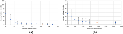
Relative error as a function of (a) replication length with 150 replications and (b) number of replications with 2,400 min replication length
Relative error as a function of (a) replication length with 150 replications and (b) number of replications with 2,400 min replication length
To perform the experiments, Arena's built-in Process Analyzer (PAN) was used. PAN allows the user to create and run multiple experiments (called ‘scenarios') automatically. The parameters used for each experiment are provided in Table 2. In Table 2, Column 1 shows the experiment number. Columns 2 and 3 show the server utilization for the TAS lane () and walk-in lane (), respectively. Columns 4 and 5 show the number of TAS lanes () and walk-in lanes (), respectively. For experiments 1, 2 and 3, the service rate is fixed at 25 trucks per hour, and is fixed at 15 trucks per hour. The arrival rates for TAS trucks () and walk-in trucks () are dependent on the value (i.e. ). In addition, the standard deviation of the interarrival time for TAS trucks and walk-in trucks were set to be the same as their interarrival time. Similarly, the standard deviation of the service time for TAS servers and walk-in servers were to be the same as their service time.
For Experiments 1 and 2, is assigned values of 0, 0.2, 0.4, 0.6 or 0.8 while is varied between 0 and 0.933 in 0.06 increments. These combinations are repeated for different values of and as shown in Table 2. For Experiment 3, and are assigned values of 0.12 and 0.133, 0.52 and 0.533 or 0.92 and 0.933, respectively, for different number of and . is varied between 1 and 9 in increment of 1.
6. Experimental results
6.1 Comparison analysis
Figure 4 shows the results of Experiments 1 and 2, combined in a way to illuminate the effect of and , on the average number of trucks per lane in the combined system. Recall that the key difference between the considered two-class queuing model and the traditional single-class queuing model is that the former allows switching. It can be observed in Figure 4 that when is low, the difference in the average number of trucks per lane between the two-class and traditional queuing system increases as is increased. To illustrate, consider the results shown in Figure 4a. When both and are approximately zero, the difference in the average number of trucks per lane between the two queuing systems is about zero. The reason is because in this situation, there is no need for TAS trucks to switch to the walk-in lane due to the lack of queue in the TAS lane. When is increased to 0.4 (TAS-lane is moderately busy) while is approximately 0 (no queue), the difference in the number of trucks per lane between the two systems is increased to 0.269, and when is increased to 0.8 (TAS-lane is extremely busy) while is approximately 0 (no queue), the difference is increased to 1.641 trucks per lane. This result can be seen in Figures 4b, 4c, 4d, 4e, and 4f as well. This finding illustrates the benefit of allowing TAS trucks to switch, particularly when the TAS lanes are busy while the walk-in lanes are not busy. The benefit of switching decreases as is increased. Take Figure 4b for example. When is 0.933 and is 0.8, the difference is only 0.013 trucks per lane. It can be seen in Figures 4a, 4b, 4c, 4d, 4e and 4f that when is close to 1, the proposed two-class queuing system with switching is equivalent to a single-class queuing system with no switching.
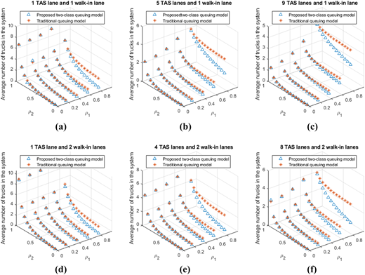
Figure 5 shows the results of Experiment 3. It can be seen in Figures 5a, 5b, 5c, 5d, 5e and 5f that the difference in the average number of trucks per lane between the two queuing systems can either increase or decrease as increases. For example, in Figure 5a when is 0.133 and is 0.92, the difference is increased from 5.0291 to 5.531 trucks per lane when is changed from 1 to 9. The rate of increase decreases as is increased. That is, the increase in the difference when is changed from 1 to 2 is larger than the increase in the difference when is changed from 8 to 9. However, in Figure 5b where is 0.92 and is 0.533, the difference is decreased from 4.006 to 3.001 when is changed from 1 to 9. This pattern can be seen in Figure 5c, 5e and 5f as well. The key takeaway from Figure 5 is that when >> , there is benefit to employing the two-class queuing system with switching. Otherwise, the benefit is minimal.
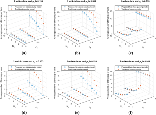
The differences in the benefit between having 1 walk-in lane and 2 walk-in lanes can be seen in the results shown in Figure 5a vs 5d, 5b vs 5e and 5c vs 5f. In Figures 5a and 5d, when is 0.133, is 0.92 and is 9, the difference is increased from 5.531 to 6.428 when is changed from 1 to 2. This result indicates that it is more beneficial to have more walk-in lanes when the TAS lanes are expected to be utilized much more heavily than the walk-in lanes. However, when is 1, the difference is decreased from 5.0291 to 3.730 when is changed from 1 to 2. Note that having two walk-in lanes is more beneficial than just one walk-in lane. However, the performance measure, trucks per lane, is lower due to the denominator being higher (3 lanes instead of 2). In Figures 5b and 5e, when is 0.533, is 0.92 and is 9, the difference is increased from 3.004 to 4.501 when is changed from 1 to 2. In this situation, it is still beneficial to have more walk-in lanes. In Figures 5c and 5f, when is 0.933, is 0.92 and is 9, the difference is decreased from 0.002 to 0.0013 when is changed from 1 to 2. In this situation, the benefit is minimal. It can be concluded that the benefit of having more walk-in lanes is reduced as the utilization of the walk-in lanes increases.
Table 3 shows the server utilization under different interarrival rates. Column 1 shows the experiment number. Column 2 shows the scenario number for Experiment 4. Columns 3 and 5 show the arrival rate of TAS trucks , respectively. The last four columns show the difference between gate utilization under the proposed queuing model and traditional queuing model. The results indicate that with the switching policy, the utilization of the walk-in server will be higher. This result corresponds to tuition. Moreover, the utilization of the TAS servers will be lower due to a small percentage of TAS trucks switching to the walk-in lane. Overall, the gate resources under the switching policy will be higher. The higher utilization is what leads to a lower waiting time for all trucks in the system.
Comparison of lane utilization under different interarrival times
| Experiment number | Scenario number | Utilization | |||||||||||||
|---|---|---|---|---|---|---|---|---|---|---|---|---|---|---|---|
| Proposed two-class queuing model | Traditional queuing model | ||||||||||||||
| TAS server | Walk-in server | TAS server | Walk-in server | ||||||||||||
| 4 | 1 | 10 | 5 | 45 | 30 | 1/10 | 1/45 | 1/5 | 1/30 | 2 | 1 | 0.19 | 0.25 | 0.22 | 0.17 |
| 4 | 2 | 15 | 5 | 45 | 30 | 1/10 | 1/45 | 1/5 | 1/30 | 2 | 1 | 0.28 | 0.32 | 0.33 | 0.17 |
| 4 | 3 | 20 | 5 | 45 | 30 | 1/10 | 1/45 | 1/5 | 1/30 | 2 | 1 | 0.36 | 0.40 | 0.44 | 0.17 |
| 4 | 4 | 25 | 5 | 45 | 30 | 1/10 | 1/45 | 1/5 | 1/30 | 2 | 1 | 0.45 | 0.48 | 0.56 | 0.17 |
| 4 | 5 | 30 | 5 | 45 | 30 | 1/10 | 1/45 | 1/5 | 1/30 | 2 | 1 | 0.54 | 0.56 | 0.66 | 0.17 |
| 4 | 6 | 35 | 5 | 45 | 30 | 1/10 | 1/45 | 1/5 | 1/30 | 2 | 1 | 0.62 | 0.62 | 0.78 | 0.17 |
| 4 | 7 | 40 | 5 | 45 | 30 | 1/10 | 1/45 | 1/5 | 1/30 | 2 | 1 | 0.71 | 0.69 | 0.89 | 0.17 |
| 4 | 8 | 40 | 10 | 45 | 30 | 1/10 | 1/45 | 1/5 | 1/30 | 2 | 1 | 0.72 | 0.73 | 0.89 | 0.33 |
| 4 | 9 | 40 | 15 | 45 | 30 | 1/10 | 1/45 | 1/5 | 1/30 | 2 | 1 | 0.78 | 0.82 | 0.89 | 0.51 |
| 4 | 10 | 40 | 20 | 45 | 30 | 1/10 | 1/45 | 1/5 | 1/30 | 2 | 1 | 0.81 | 0.88 | 0.89 | 0.67 |
| 4 | 11 | 40 | 25 | 45 | 30 | 1/10 | 1/45 | 1/5 | 1/30 | 2 | 1 | 0.85 | 0.95 | 0.89 | 0.83 |
6.2 Approximation equations
While DES models can be used to model any degree of complexity in truck queuing at the terminal gate, its development, calibration and validation require extensive data, time and modeling expertise (Caro and Möller, 2016). To facilitate the use of the simulation results, regression models are developed. Many previous studies have used this approach (e.g. Jackson and Pollock, 1978; Mifflin et al., 1990), that is, they developed regression models using simulation results to facilitate prediction of an outcome variable. In this study, the aim is to facilitate the prediction of the average number of trucks waiting in each lane. Various regression model specifications, including both linear and non-linear, were tested, and the best fit ones are shown in the following equations. The nonlinear specifications were based on the work of Jackson and Pollock (1978) and Mifflin et al. (1990). It should be noted that the developed regression models have adequate sample size based on Montenegro’s (2001) guideline of at least ten observations per number of independent variables.
Equation (1) can be used to obtain the average number of trucks waiting in each lane when the number of walk-in lane is 1, and Equation (2) can be used to obtain the average truck queuing time when the number of walk-in lane is 1.
where
average truck queue length when there is 1 walk-in lane,
average truck queuing time when there is 1 walk-in lane,
arrival rate of TAS trucks (trucks/hour),
arrival rate of walk-in trucks (trucks/hour),
service rate of TAS trucks (trucks/hour),
service rate of walk-in trucks (trucks/hour),
the variance of the arrival rate for TAS trucks,
the variance of the service rate for TAS trucks,
the variance of the arrival rate for walk-in trucks and
the variance of the service rate for walk-in trucks.
number of TAS lanes, between 1 and 9.
When the number of walk-in lanes () is 2, Equations (3) and (4) should be used instead of Equations (1) and (2).
where
average truck queue length when there are 2 walk-in lanes and
average truck queuing time when there are 2 walk-in lanes.
To illustrate how the developed approximation equations can be used, consider the scenario where a terminal operator is considering adding one walk-in lane to accommodate walk-in trucks; as discussed, it would not be appropriate to allow these trucks in the TAS-lanes because their service times could be exceedingly high due to the lack of paperwork preclearance. Suppose the number of TAS-lanes is 5, is 0.8 ( = 32 trucks per hour and = 40 trucks per hour), = = 2, = = 1 and is 0.3 ( = 9 trucks per hour and = 30 trucks per hour), applying Equation (1), we get 2.38 trucks, compared to 4.95 trucks when there is 1 walk-in lane but no switching is allowed. If two walk-in lanes are considered, then the average queue length will be 1.22 trucks (Equation (3), compared to 4.8 trucks without switching). While the findings to this example are obvious, adding extra lane(s) will result in lower truck waiting time, it illustrates a new capability not available before.
A not-so-obvious example is when the terminal operator has to decide whether to convert one of the current TAS-lanes to a walk-in lane. Suppose there are currently 5 TAS-lanes, and the question is whether the trucks are better off in a 4 TAS-lanes to 1 walk-in lane setup. If is 0.6 ( = 24 trucks per hour and = 40 trucks per hour), = = = = 1 and is 0.5 ( = 15 trucks per hour and = 30 trucks per hour), then the 4-to-1 setup is more beneficial than the 5-to-0 setup, a savings of 0.05 trucks in the queue. This example demonstrates the benefit of the considered two-class queuing model with switching.
The proposed two-class queuing model with switching could potentially benefit all trucks. That is, in practice, the walk-in trucks and the TAS trucks that arrived earlier than their assigned time slot cannot get service from a TAS lane. In the proposed two-class queuing system, it not only allows walk-in trucks to receive service without affecting the upcoming TAS trucks but also get the trucks with appointments which arrived ahead of time into the port. The broader significance of this study is that it may lead to a design change in the physical layout of future terminals/ports to have separate service lanes for different types of services and to allow trucks to switch to lanes.
7. Summary and conclusions
This paper considered a two-class queuing system where TAS trucks will switch to a walk-in lane upon arrival if all the TAS-lanes have queues and all TAS-lane servers are occupied, and the walk-in lane queue is empty, and its server is idle. It is different from all previous work in two key aspects: (1) it is the first container terminal study to consider more than one entity and server class and (2) it is the first study to consider a multi-class queuing system that allows entities (i.e. trucks) to switch servers. This considered queuing system is mathematically shown to be stationary using a theorem developed by Resnick (1992). Establishing the stationary property for the proposed queuing strategy is necessary because without this property, the queuing system would never reach steady state and it could lead to infinite queuing. Due to the complexity of the model, a DES model was used to obtain the average truck queue length and average truck queuing time for both TAS lanes and walk-in lanes. The experiment results, using data previously derived from terminals and reported in previous studies, indicated that the proposed queuing model is most beneficial when the utilization of the TAS lanes is expected to be much higher than that of the walk-in lanes. To facilitate the application of the proposed model, approximation equations are provided for calculating the average truck queue length and average truck queuing time. The approximation equations allow terminal operators and planners to easily evaluate different gate designs.
The considered queuing system makes an important contribution to the field. It, however, has several shortcomings that need to be addressed in future research to make it even more practical. Switching is only allowed upon arrival. Future work could consider allowing trucks already in queue to switch, provided there is sufficient space to do so. The extension could consider switching to a walk-in lane or another TAS lane. The derivation of stationary property assumed truck arrivals to be Poisson distributed and service times to be exponentially distributed. Future work could extend the derivation to consider other types of distributions. Lastly, the provided approximation equations are limited to nine TAS lanes and two walk-in lanes. Future work could seek to provide a greater of number of combinations and perhaps with more classes.
