Exploiting digitalisation to plan interventions on large water distribution networks Open Access

Modern societies have grown accustomed to reliable and affordable access to potable, pressurised water in sufficient quantity. This essential service depends on infrastructure managers, who plan and execute corrective and preventive interventions on network components to maintain an adequate level of service. This is a challenging task due to the spatial extent of large networks, limited financial resources and the complexity of coordinating interventions with multiple stakeholders.

Ideally, the decision space of intervention alternatives would be formally defined and a quantitative cost–benefit analysis would be performed. Infrastructure managers could then determine the optimal intervention programme – that is, the set of interventions that results in the highest net benefit while respecting all considered constraints. The end result would be a consistent approach to intervention planning that would be transparent to stakeholders. In reality, time pressure and the complexity of the problem often lead infrastructure managers to rely on intuition and experience (van Riel et al., 2014, 2016).

This is not ideal for a number of reasons. First and foremost, stakeholders expect transparency in decision-making. Secondly, knowledge transfer to the next generation of decision makers is inevitably affected. Thirdly, experts have been shown to make inconsistent decisions (Kahneman and Klein, 2009). Finally, intuition within the infrastructure-management context cannot be considered skilled due to a lack of available cues needed to indicate that a given decision was indeed better than other alternatives (van Riel et al., 2014). In other words, it is difficult to evaluate an executed intervention because the effect on network performance will not always be observable. In addition, infrastructure generally outlasts the professional careers of infrastructure managers. Furthermore, decisions are generally not recorded in a format that would allow periodical retrospective evaluation. Without these prerequisites, skilled intuition cannot be developed.

That being said, there are obstacles to implementing a consistent and transparent intervention-planning methodology that must first be overcome. The size of modern water distribution networks (WDNs) results in an immense number of theoretically possible intervention programmes. Evaluating these alternatives exhaustively is often impractical due to the associated computational effort. Additionally, decision makers are interested in investigating sources of uncertainty, which requires performing numerous analyses in a reasonable time period. Examples of such sources of uncertainty include the models used to calculate the costs and benefits of executing preventive interventions, the associated model parameters and how these will change in the future due to socio-economic trends, climate change and technological innovation.

Digitalisation can be leveraged to this end. The enhanced ability to collect, store and analyse data to produce useful information has far-reaching implications in decision-making. Although digitalisation has already had profound effects on infrastructure, it is lagging compared with other sectors of the economy. Concrete examples are needed to illustrate how digitalisation can be further exploited in intervention planning.

This paper addresses this gap in a practical manner by discussing the simplifications made to the methodology presented by Kerwin and Adey (2020). The relationship between runtime and decision variables is explored, and three applications of the methodology to intervention planning are presented: (a) estimating the budget requirements needed to implement various intervention strategies, (b) communicating the trade-offs of different strategies and budget scenarios and (c) investigating how the intervention-planning activities of other networks could affect these estimations.

In this section, a brief summary of the methodology presented by Kerwin and Adey (2020) is first provided. This is followed by a general discussion of the simplifications made to scale the methodology up to a significantly larger network.

Kerwin and Adey (2020) proposed an intervention-planning methodology that incorporates both buried pipes and facility-housed components, utility defined strategies and operational and financial constraints. The methodology is summarised in the following five steps.

• Model the network, failures and preventive interventions.

• Define intervention strategies.

• Identify intervention candidates.

• Perform a cost–benefit analysis.

• Optimise within constraints.

The first step is to describe the network at the level of detail at which interventions are executed (i.e. the object level). This is done by categorising objects using appropriate attributes on function, dimension, composition and vintage. For all defined categories, models are needed to quantify failure in terms of risk as well as estimate the costs and benefits of intervention execution. Then, intervention strategies are defined by the utility for all categories that require preventive intervention planning. Categories that are only managed with corrective strategies are thus excluded. These preventive intervention strategies represent how these infrastructure assets should ideally be managed without considering constraints, network properties or economies of scale. Whole-life cycle costing is used with an appropriate discount rate to determine these strategies. A strategy consists of an object category, its environment, an intervention-triggering criterion (e.g. age and failure rate) and the intervention type to execute. Once defined, these strategies are used to identify intervention candidates for the next short-term intervention-planning period. To consider the cost-saving potential of economies of scale, grouping rules are defined for combining intervention candidates with other spatially proximate or functionally similar objects. A cost–benefit analysis is performed on the considered intervention types that could be executed on the intervention candidates and derived groupings. These results are used in a two-step optimisation algorithm to determine the set of intervention candidates that should be executed in the next 5-year period, given a list of operational and financial constraints.

This intervention-planning methodology is novel in that it combines both buried pipes and facility-housed objects and considers a variety of ways in which intervention strategies could be defined as well as the influence of economies of scale in a monetised cost–benefit analysis framework. Ideally, this paper would include a rigorous comparative study of intervention-planning methodologies used by utilities and consulting firms in the water sector. However, due to reasons of confidentiality, data security and industry competition, finding this level of openness is difficult in practice.

Despite the widespread and relatively affordable access to powerful computational infrastructure, infrastructure managers must inevitably employ numerous simplifications to model large networks. Enumeration of the potential combinations of network component groupings, intervention types and intervention timings results in a combinatorial explosion as the network size increases. The reduction in the spatial and temporal complexity of the problem and associated computational effort must be done in a manner that maintains an adequate description of important problem elements so that useful insights can be gained. Previous examples of approaches used to model large networks include the development of surrogate models (Balekelayi and Tesfamariam, 2019), leveraging parallel computing configurations (Alvarruiz et al., 2017) and the use of efficient heuristics to solve optimisation problems such as evolutionary algorithms (Nicklow et al., 2010). In this paper, the planning complexity is simplified at three levels: definition of decision variables, selection of models and consideration of constraints.

A decision variable refers to a permissible intervention type that could be executed on a network component or a grouping of components at a specified moment in time. These are based on the existing network configuration (i.e. topology and component dimensions). In other words, decision variables representing network expansion (e.g. additional pumping station) or operation optimisation (e.g. network partitioning with additional isolation valves) are not considered. Such interventions improve the level of service (e.g. reduced leakage) and result from a top-down planning process where problems are identified from network performance indicators (e.g. leakage rate) and possible solutions are generated and evaluated. This is complementary to the proposed bottom-up approach but outside of the scope of this paper.

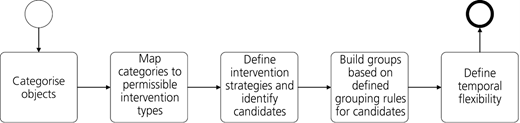
It is necessary to define explicitly the decision space so that stakeholders understand which intervention alternatives are considered and how they are evaluated. Inevitably, simplifying assumptions are needed and must be clearly stated. The process in Figure 1 is used for decision variable simplification using Business Process Model and Notation (BPMN) 2.0 (Allweyer, 2010).

Firstly, the network is categorised using physical, operational and environmental attributes relevant for intervention planning. For objects housed in facilities, this is a straightforward endeavour. The distribution network requires an aggregation step to convert segments into pipe decision variables. Typically, physical and operational properties are used such as material, diameter, installation year and subnetwork (Kerwin and Adey, 2020). However, examples of additional criteria exist such as road intersections (Mailhot et al., 2000) or isolation valves (Giustolisi and Savic, 2010; Walski, 1993). In addition, service lines and other pipe appurtenances (e.g. valves, hydrants) can be either considered as separate categories or agglomerated into the associated water main as a simplification (FCM and NRC, 2003a). In the paper by Kerwin and Adey (2020), service lines were considered separately. In this paper, they are agglomerated into the associated water main.

Secondly, the defined categories are mapped to permissible intervention types. There exist a great number of potential interventions that could be executed per object category. For example, reservoir rehabilitation techniques include cement–mortar coating, polymer coating, relining with polyethylene plates or ceramic tiles and so on. These techniques vary in cost, maintainability, longevity and sensitivity to water composition. This variability in intervention techniques exists for pipes (AWWA, 2014) and other object categories. The choice of specific permissible intervention techniques depends on the technical limitations of the technique (e.g. limited pipe diameter range), applicable best practice guidelines, the expertise of local contractors and the experience of the utility.

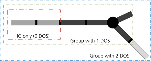
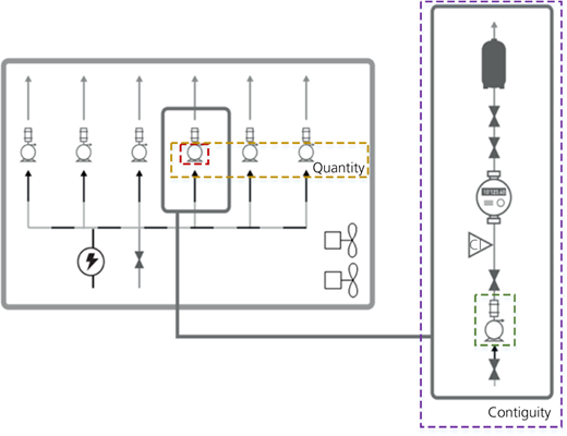
Next, intervention strategies are defined for all categories and used to identify intervention candidates. The intervention-triggering criteria will depend on the specific object category, the available data, the best practice guidelines and the risk tolerance and preferences of the utility. For example, a threshold failure rate may be used as a guideline for the replacement of pipes (DVGW, 2006; SVGW, 2012; Walski and Pelliccia, 1982), whereas for pump motors, operating hour thresholds provided by the manufacturer may be preferable. These strategies are used to identify intervention candidates in the network. The decision space of alternatives is thereby reduced to these candidates and their derived groupings. Groupings are essential for considering the cost-saving potential of economies of scale. Cost savings arise from contractor discounts on large interventions, manufacturer discounts on large equipment orders or lower fixed costs (intervention set-up, mobilisation, reduced downtime etc.). This is particularly advantageous for large utilities, which can benefit from reduced unit costs. Defined grouping rules are used to control the associated increase in decision variables. Table 1 lists example grouping rules. In the paper by Kerwin and Adey (2020), the only grouping rule used was pipe contiguity to a degree of separation (DOS) of one. The grouping rules used in this work are facility contiguity for pumps and pipe contiguity to a DOS of two.

Figures 2 and 3 show the grouping process for pipes and facility objects.

As municipal utility networks are generally spatially proximate, the intervention-planning activities of one network will affect the costs and benefits of executing interventions on other networks. Ideally, this would be reflected in the grouping rules but is currently impractical due to existing organisational structures (i.e. infrastructure networks are managed by separate organisations with different financial and operational objectives).

Finally, temporal considerations are reduced by assuming that intervention timing is flexible and can be postponed by a year or until the next short-term (i.e. 5-year) planning period to comply with budget limits. Exceptions include priority interventions and coordination interventions. Priority interventions are interventions defined by the infrastructure manager that must take place in a specified year. Coordination interventions are those initiated by other utility networks (roads, sewers etc.) that will either take place in the year of planned coordination or not at all due to cost–benefit considerations or budget constraints.

Once the decision space has been defined, models are needed to calculate the associated costs and benefits of preventive intervention execution using a common metric (i.e. monetary units). Often simulation-based models are used to calculate the impacts from preventive interventions (e.g. impact on traffic circulation (Lee, 2009)) or to estimate failure risk (e.g. service interruption following failure through the use of extended period hydraulic simulation (Giustolisi, 2020; Giustolisi and Walski, 2012)). Such models allow improved uncertainty quantification. However, when coupled with an optimisation framework, where many evaluations are needed, the required computational effort can be prohibitive (Sirsant and Reddy, 2020). Instead of computationally demanding simulation-based approaches, deterministic models were developed using historical operating data, spatial data from geographic information system (GIS) databases and the expert knowledge of utility workers.

Costs are estimated by first identifying affected stakeholders (e.g. utility, consumers and commuters), the expected impacts (e.g. excavation costs, traffic diversion and temporary service interruption), relevant attributes (e.g. zoning, average daily traffic load and number of service lines) and selection of appropriate models for monetisation. The monetisation of intangible impacts (e.g. longer commute to work during construction work) is difficult in the absence of a marketplace. Approaches exist such as willingness-to-pay surveys and cost inference from lost economic output but have their limitations. For example, survey participants often contradict their statements (i.e. willingness to pay) with their actions (i.e. revealed preference). Nonetheless, selecting imperfect monetisation models for these impacts is preferable to ignoring them, which implies that these impacts have no value.

The benefit of executing an intervention is proportional to the associated improvement in the level of service, but service is provided by the network and interventions are executed on individual objects. Thus, a method is required to estimate incremental service improvement in order to compare intervention alternatives. This is not straightforward, as service improvement may not be easily observable or may require a lengthy subsequent monitoring period during which many other interventions will have been executed.

The approach taken is to estimate failure risk and the expected short-term risk reduction that would be achieved by executing the preventive intervention within the planning period, where risk is the product of failure probability and monetised failure consequence. There exist numerous approaches for calculating risk (Francisque et al., 2014; Kabir, 2016; Kabir et al., 2015; Shahata and Zayed, 2015). The chosen approach is to calculate the risk to stakeholders (utility and consumers) assuming that objects fail individually. Thus, multiple or cascading failures (Berardi et al., 2014, Laucelli and Giustolisi, 2014) are not considered. Risk reduction is estimated using intervention-specific factors ranging from 1 (complete reduction, i.e. replacement) to 0 (i.e. nothing done). These factors estimate the associated decrease in failure probability resulting from intervention execution. Interventions can also reduce risk by decreasing the expected failure consequences. For example, the adoption of machine learning algorithms to detect pipe bursts can lead to faster response times for corrective interventions. These algorithms monitor and instantly identify anomalies in network pressure data, thereby limiting the failure consequences (Jung et al., 2015; Romano et al., 2014; Wang et al., 2020). Such interventions are not considered.

Currently, the intervention-specific risk reduction factors are based on expert opinion. Most related scientific literature focuses on intervention effectiveness (i.e. improvement of a key condition indicator), primarily on pavement infrastructure (Khurshid et al., 2009; Labi and Sinha, 2003a, 2004; Labi et al., 2007), with comparatively little existing for municipal pipe networks (Lin et al., 2019). In describing intervention effectiveness for pavement systems, Labi and Sinha (2003b) discuss three possible measurements: instantaneous performance jump, deterioration level reduction and deterioration rate reduction. This is equally applicable to water infrastructure. Consider a leaky metallic water main. The installation of a repair clamp to fix a pinhole leak caused by corrosion results in an immediate decrease in leakage and increase in pressure (performance jump). However, the underlying issue of corrosion is not addressed, so the deterioration level and rate remain unaffected. If cathodic protection is applied along with the repair clamp, there will be an additional reduction in the deterioration rate but not the deterioration level (the existing corrosion pit depth is unaffected). If a structural relining intervention is executed at some later point following the repair clamp, there will be a performance jump and reduction in the deterioration level and rate due to the enhancement in structural integrity. In practice, these data are difficult to measure, as regular inspection of buried pipes is cumbersome and expensive or requires long observation periods before changes in relevant performance indicators (e.g. failure rate) become apparent. Additional research is required to derive factors quantitatively from observable performance indicators. Tables 2 and 3 list the costs and benefits of intervention execution along with relevant attributes, which are considered in the paper. More information can be found in the paper by Kerwin and Adey (2020).

In practice, resources are almost always constrained and certain interventions must be executed within a specified time window. Given insufficient resources, certain interventions will be inevitably postponed. Appropriate algorithms are thus needed to determine the set of interventions that should be executed in the planning period of 5 years given a list of operational, financial or temporal constraints. To reduce complexity, spatial and temporal constraints are considered sequentially, which greatly shrinks the search space. This simplification is based on the assumption that the costs and benefits of preventive intervention execution do not change from 1 year to the next within the planning period of 5 years.

Spatial constraints are accounted for using the branch-and-bound method with an objective function of maximising net benefit. This is calculated as the difference between intervention benefits and costs. Implementation is done with the R software package (R Core Team, 2013) with the lpSolveAPI package (Konis and Schwendinger, 2014). This results in the optimal configuration (i.e. spatial grouping and intervention type) for all intervention candidates. Next, the temporal constraints are considered such as intervention timing and annual budget limits. The allocation algorithm is illustrated using the BPMN process diagram in Figure 4.

Firstly, priority interventions (i.e. interventions that must be executed) are assigned to their specified years. If the budget limits are insufficient to execute all priority interventions, then an error message is returned. Secondly, coordination interventions are considered. If the budget is insufficient, then dynamic programming (modelled on the 0–1 knapsack problem (Toth, 1980)) is performed. Finally, all remaining interventions are considered. Again, if the budget is insufficient, dynamic programming is used for optimal allocation. For very large problem instances, runtimes for the knapsack optimisation with dynamic programming can become cumbersome (Wojtczak, 2018). The relationship between runtime and budget constraints for the case study is explored in the next section. Depending on the needs of infrastructure managers, it may be acceptable to sacrifice the optimality of the dynamic programming result for a faster, potentially non-optimal result using a heuristic such as greedy local optimisation.

Table 4 lists the considered constraints. More information on the constraints considered in this paper as well as optimisation methods used in other studies on intervention planning can be found in the paper by Kerwin and Adey (2020).

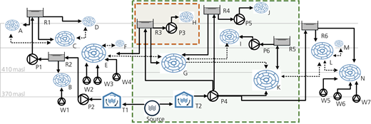
The case study consists of data obtained from a large WDN. All provided data such as network configuration, dimensions and other attributes have been modified for reasons of confidentiality. An approximate elevation diagram (see Figure 5) is used to show the layout of the different subnetworks and facilities. The diagram begins at the source and branches off to two treatment stations. In total, there are 14 subnetworks, six pumping stations, seven groundwater-pumping wells, six reservoirs and two treatment stations. These have been labelled from left to right as follows: treatment stations with a T, pumping stations with a P, groundwater wells with a W, reservoirs with an R and subnetworks with a single unique letter. Internetwork connections are denoted with a dotted line.

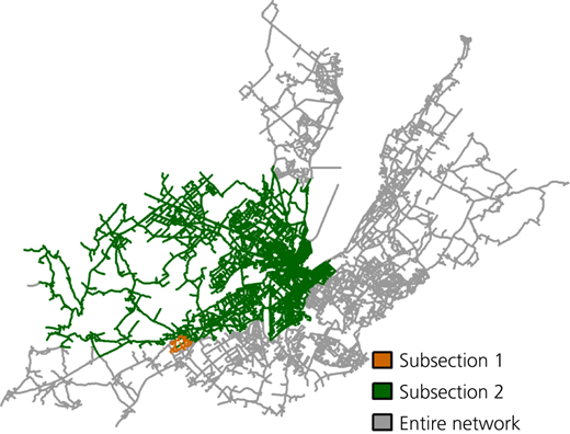
To investigate the relationship between runtime and decision variables, the methodology is run using three subsections of the network. The smallest subsection (shown with the orange dashed line in Figure 5) consists of a subnetwork, a reservoir and a pumping station and was used as the case study in the paper by Kerwin and Adey (2020). The second subsection (shown with the green dashed line in Figure 5) consists of five subnetworks, three reservoirs, four pumping stations and a treatment centre. The third one encompasses the entire network in Figure 5. Figure 6 shows the corresponding geographic extent of the subsections. The runtimes of the analyses are then plotted against decision variables (see Figure 7).

Tables 5 and 6 provide additional summarising data on the subnetworks and facilities. In Table 5, the theoretical supply capacity, projected max. hourly demand and water usage profile are used to estimate impacts to service provision following a failure. The theoretical supply capacity is estimated by considering each subnetwork separately, identifying the possible ways in which the subnetwork could be supplied and using historical operation data to estimate hourly flows. The projected max. hourly demand refers to the maximum expected hourly demand under normal operating conditions and peak-seasonal conditions. This value is estimated using historical consumption data and short-term demographic projections. The water usage profile is estimated from zoning information, the number of service lines and the seasonal variation in daily water demand profile. In Table 6, the facility configuration provides information on the number of independent processes in each facility and total facility output.

The facility and pipe contiguity rules are used to build groupings for pumps and pipes, respectively (see Table 1). A maximum DOS of two is used for pipes. Table 7 contains the quantity discounts applied to large pipe interventions above certain cost thresholds. These depend on intervention type. All contractors can carry out open-trench replacements, as this is the traditional technique used in the industry. The other trenchless techniques require additional specialised knowledge and equipment and are generally offered by fewer contractors. Thus, contractors are expected to offer higher discounts on open-trench replacements than other intervention types in order to remain competitive. Furthermore, trenchless techniques are not considered on groupings less than 100 m long or containing pipe objects with a density of service lines greater than 20 per 100 m. Above this service line density, it becomes more economical to simply execute an open-trench replacement on the water main (FCM and NRC, 2003b). Monetary units (mu) and kilo monetary units (kmu) are used throughout this paper when quantifying cost and risk.

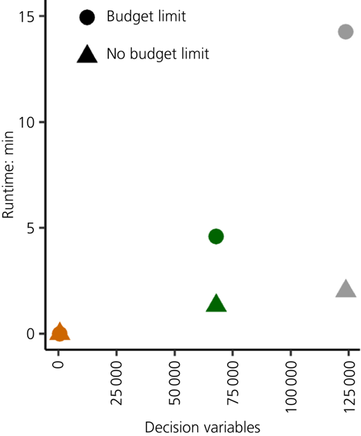
Figure 7 contains the runtimes for the three different WDN sections. The analysis was performed on a Lenovo ThinkPad computer (Intel Core i7-8650U central processing unit at 2.11 GHz, 16 GB random-access memory). The colours of the points correspond to the colours used in Figures 5 and 6 to denote network subsections. The optimisation was done under both a constrained-budget scenario and an unconstrained-budget scenario. When the budget is unconstrained (no budget limit in Figure 7), the runtime increases linearly with the number of decision variables. In contrast, the runtime increases exponentially with the number of decision variables under a constrained-budget scenario (budget limit in Figure 7) due to the additional effort needed to run the dynamic programming algorithm. The runtimes and decision variables can be found in Table 8.

From Figure 7, it is evident that the runtime increases linearly with the number of decision variables in the unconstrained-budget scenario. This is a useful realisation, as many questions of interest can be answered without consideration of budget constraints and applied to much larger decision problems. Two examples of such questions are shown in the next section. The first is estimating the short-term budget requirements needed under different intervention strategies. The second is investigating how the intervention-planning activities of other networks could affect these estimations. The latter question is a topic of increasing interest in Switzerland (Hensel et al., 2018, Zuleger and Herlyn, 2016, 2019), as infrastructure managers are under increasing pressure to coordinate preventive interventions and minimise future societal impacts. Hensel et al. (2018) reported that an analysis of past budget spending (2012–2016 in Zurich) found that roughly 50% of planned interventions could not be executed according to schedule due to the sudden financial requirements of unexpected coordination interventions.

In this section, three applications of the methodology are presented to highlight the advantages of consistent and transparent intervention planning facilitated by digitalisation. These applications are (a) estimating the budget requirements of implementing various intervention strategies, (b) communicating how investments are being directed throughout the network under different strategies and budget scenarios and (c) exploring how budget estimates could be affected by the intervention-planning activities of other networks.

Water utilities employ different intervention strategies depending on risk tolerance, data availability, stakeholder preferences and other factors. It is useful to evaluate and compare quickly the corresponding budget requirements of different strategies in a consistent manner. Table 9 lists the parameters of three intervention programmes (IP1, IP2, IP3) that were determined using different age- and risk-based strategies. No budget limit was used.

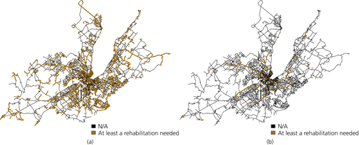
The intervention candidates will vary drastically depending on the defined strategies. Figure 8 visually highlights the difference between intervention candidates (shown in brown) of IP1 (age-based strategies) and IP2 (risk-based strategies). All intervention candidates require at least a rehabilitation intervention as per the strategies listed in Table 9. The candidates of IP3 are a combination of both IP1 and IP2 and thus, for reasons of simplicity, are not shown.

From Figure 8, it is evident that the age-based strategies used in IP1 result in far more intervention candidates than the risk-based ones of IP2. The visible intervention candidates for IP2 (risk-based) strategies are predominately transmission pipes concentrated in areas of high economic output.

Once the intervention candidates have been identified, the cost–benefit analysis and optimisation steps are performed. The runtime for each intervention programme was less than 2 min. The results of the three intervention programmes are summarised in Table 10.

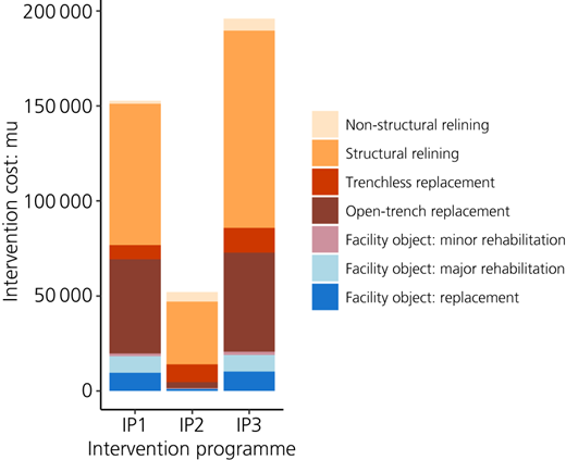
The 5-year intervention costs of implementing the strategies described in Table 9 are 152.8, 52.1 and 196.0 kmu, respectively. The cost of intervention execution is almost three times larger for IP1 compared with that for IP2. However, IP2 results in significantly more traffic disruption costs. The resulting levels of risk reduction are very similar for the two. Overall, the net benefit is highest for IP1, followed by that of IP3. This parameter is the difference between risk reduction and total intervention costs, where intervention costs consist of both the direct costs and indirect costs (traffic and service interruption) of executing interventions. This result depends heavily on the thresholds used in the age- and risk-based strategies and should not be construed as a finding that can be generalised (i.e. age-based strategies are better than risk-based ones).

Figure 9 provides additional information on the intervention costs of the three intervention programmes by intervention type. Such comparison diagrams are useful for communicating with stakeholders how investments into water infrastructure are being directed.

In Table 10, the parameter, number of projects, refers to the number of separate interventions executed over the 5-year period. Vastly more projects are executed when age-based strategies are used compared with risk-based ones. The largest difference is in the number of interventions executed on facility objects. Facilities are designed with a certain level of redundancy so that maintenance work can be done without disturbing service. Thus, in general, the consequences of failure are lower for facility objects than for distribution or transmission pipes. For this reason, fewer facility objects met the risk threshold of 100 mu used in IP2 to identify intervention candidates. Risk-based strategies resulted in the inclusion of significantly more transmission pipes. This is to be expected, considering the potentially catastrophic consequences that can occur when such pipes fail. IP3 combines the age and risk strategies of IP1 and IP2; however, the number of projects in IP3 is lower than the sum of IP1 and IP2. This occurs because there is a certain overlap of intervention candidates that appear in both IP1 and IP2. A more detailed network- and facility-level breakdown of projects is provided in the next section.

For increased transparency, a network- or facility-level breakdown of intervention projects is a preferred level of detail. At this level, it is possible to explain where investments are being directed in the WDN under different intervention strategies and communicate to stakeholders the impacts of budget restrictions on these investments. When budgets are limited, infrastructure managers must decide which interventions to execute and which ones to postpone. This requires an objective metric and a suitable algorithm for consistent and transparent decision-making. In this section, monetised net benefit and dynamic programming are used to answer these questions.

A project-level comparison of four different intervention programmes is provided. These intervention programmes are generated using the strategies of IP2 and IP3 (see Table 9) under a constrained- and an unconstrained-budget scenario. An annual budget limit of 8 kmu (40 kmu over 5 years) is applied in the constrained-budget scenario.

Tables 11 and 12 provide project-level comparisons of interventions executed in facilities and subnetworks, respectively, for the four intervention programmes.

The risk-based strategies of IP2 resulted in more than twice as many pipe projects compared with facility projects. These projects are concentrated in subnetworks G and K. Subnetwork G services a densely populated area with important centres of economic activity. Subnetwork K corresponds to the downtown core, which is the most dense and economically important part of the city. Subnetwork K also contains many of the oldest pipes in the WDN, which explains why most interventions are executed in this subnetwork when risk-based strategies are used.

In contrast, several subnetworks had no interventions. Subnetworks A, B, D and H had zero interventions when only risk strategies were used. These subnetworks represent more recent additions to the WDN, and in general, the pipes are in good condition. Furthermore, these subnetworks service rural, low-population-density villages, which contribute to a lower failure risk compared with subnetworks G and K.

For facilities, risk strategies resulted in relatively few interventions. This is to be expected due to the high level of redundancy that is built into these facilities. The facility with the largest number of interventions with risk strategies was P4. This is a very large pumping station that supplies water to multiple subnetworks. These interventions were mostly on critical valves and equipment essential for process automation and control.

When age and risk strategies are used (IP3), there are a considerable number of interventions distributed throughout the facilities and subnetworks. Inside the facilities, these interventions were mostly on sensors and measuring equipment. No interventions are executed in reservoirs R3 and R4, as these were recently rehabilitated.

When a budget limit is applied, the effect is most evident on the interventions executed on the subnetworks. In general, the net benefit of the facility interventions is higher. This is due to the fact that facility objects have shorter service lives compared with buried pipes and must be replaced or rehabilitated more often. In addition, the costs of executing interventions on facility objects are lower. There are no impacts to traffic and service interruption to clients, and the actual cost of intervention execution is typically lower than that of excavating buried pipes. This results in a higher net benefit than pipe interventions. In general, the condition of the buried pipes is reasonable and failure rates are moderate, as pipes have been consistently replaced at a relatively high rate over the past several decades.

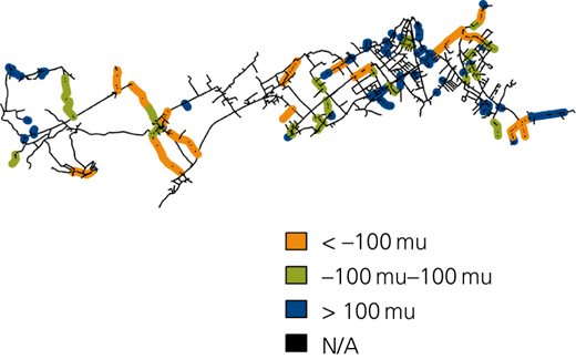
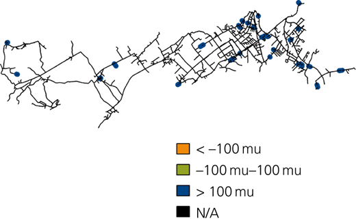
Figures 10 and 11 show the effects of the budget limits on pipe interventions for subnetwork E, with the intervention strategies of IP3 (age and risk based). Interventions are coloured by net benefit. In Figure 10, no budget limit is imposed and interventions range from 15 to 1287 m long with an average of 223 m. In Figure 11, interventions range from 15 to 163 m long, with an average of 57 m. The figures clearly show that when budgets are limited, the interventions with low net benefit are postponed to the next planning period.

The previously described intervention programmes do not consider the potential influence of interventions executed on other infrastructure networks. These interventions will affect the cost–benefit analysis, as it becomes possible to execute a replacement intervention (i.e. open-trench replacement) at a lower cost. At the same time, if the water utility does not join the other infrastructure network in coordination, the risk of failure increases due to excavation works in the immediate vicinity. Thus, there is a considerable incentive to replace pipes earlier than one normally would in such circumstances. Such interventions are often difficult to foresee and are sometimes announced only a few months in advance.

To estimate the potential influence of such interventions on budget estimates, the cost–benefit analysis is modified using coordination factors (see Table 13). These factors depend on the relative depth of the infrastructure of the coordinating utility (Kerwin and Adey, 2020). Infrastructure located above water pipes, such as the road surface, has a lower potential for cost reduction than sewer pipes, which are buried below. Similarly, the failure risk of a water main increases substantially if a sewer replacement intervention is being executed compared with a road-resurfacing project.

Next, additional intervention strategies are defined for pipes located in coordination areas. Finally, stochastic simulation is performed. The intervention-planning methodology is run a number of times, and each time a defined number of coordination opportunities are randomly allocated to pipes over the planning period.

Of course, the resulting impact to the budget estimates is heavily dependent on the values of the coordination factors, the thresholds used in the additional strategies and the number of randomly allocated coordination opportunities. Below, the influence of the thresholds used in strategies as well as the number of allocated coordination opportunities are investigated.

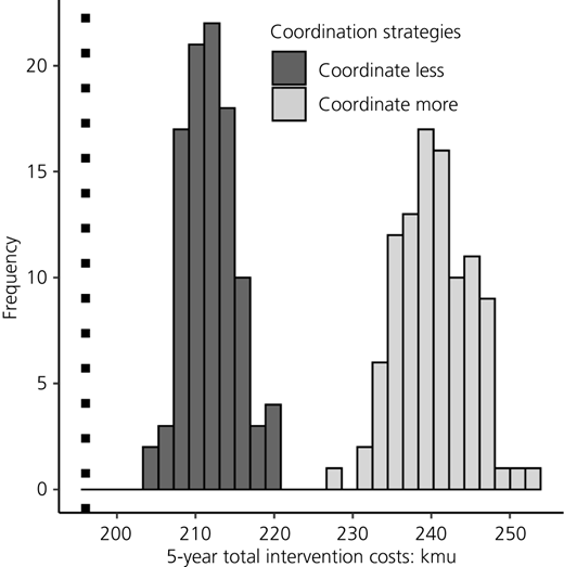
Table 14 contains the parameters used in the stochastic simulations with varying age and risk thresholds for pipes in coordination areas. In addition to the age- and risk-based strategies defined in IP3 (see Table 9), additional coordination strategies are defined. The coordination strategies used in simulation 1 (S1) are summarised as more risk tolerant with the water utility less likely to coordinate, whereas simulation 2 (S2) represents a more risk-averse approach with more coordination. Each simulation consisted of 100 runs of the methodology and took approximately 3.5 h on the previously described Lenovo ThinkPad computer.

Figure 12 visualises the results of the two simulations in terms of the 5-year cost of intervention execution. The cost of IP3 (see Table 10) is shown as a dotted black line for reference.

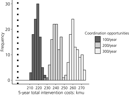
Next, the influence of the number of coordination opportunities is explored (Table 15). The strategies of S2 (coordinate more) are used.

Figure 13 shows the spread of the 5-year cost of intervention execution of the three simulations. Again, the cost of IP3 (see Table 10) is shown as a dotted black line for reference.

The results of the simulations are summarised in Table 16.

The results of the simulations show that the intervention activities of other networks have a considerable influence on short-term budget estimates and should not be ignored. Consider the results of S1 and S4, which represent the low and high scenarios, respectively. Under the parameters of S1, the 5-year budget increased by 8.1% on average, compared with that of the reference intervention programme (IP3). This increased to 33.7% for S4, where strategies promoting coordination are used and 300 coordination opportunities are expected per year.

This paper builds on the work presented by Kerwin and Adey (2020). The simplifications made to model the much larger network shown in the case study are explained in general terms. The approach consists of reducing the number of decision variables, selecting deterministic models for calculating the costs and benefits of executing interventions and sequentially considering constraints in the optimisation. The relationship between runtime, decision variables and budget constraints is explored. This is done by dividing the case study WDN into three subsections of increasing size and running the analysis. The runtime increased linearly with larger instances of decision variables for the unconstrained-budget scenarios. This is a clear indication that the methodology could be applied to much larger networks. Although the runtime does increase exponentially with a budget constraint, the current runtime of 14 min is likely acceptable for a large network for most applications.

Three potential applications are shown of questions that could be answered by the methodology. Two of these do not require a budget constraint. The first is determining the short-term budget requirements associated with a set of defined intervention strategies. This is useful for communicating to stakeholders how assets are managed and justifying one set of strategies over another. The second application involves communicating the project-level trade-offs of implementing different intervention strategies or budget scenarios. Defined intervention strategies make it easy to provide justification for the inclusion of certain objects in the final intervention programme. In the event of limited financial resources, the net benefit provides a clear explanation for the interventions that are postponed to the next planning period. The third is investigating how these short-term budget estimates could be affected by the unforeseeable intervention-planning activities of other networks. Infrastructure managers are under increasing pressure to coordinate interventions with other utilities to avoid future service disruptions and traffic impacts. Thus, budget estimates can be updated based on the results of stochastic simulations of the intervention activities of other networks. This information can be used to communicate to politicians the budget needs associated with increased coordination.

The scenarios presented in this paper are simplistic compared with funding submissions that infrastructure managers must prepare in the real world and are solely meant to communicate the utility of the methodology. In practice, detailed stakeholder surveys are needed to characterise adequately the needs and preferences of the served population and studies must be done to analyse demographic, climate and regulatory trends.

For reasons of scope, a detailed discussion of how intervention strategies are determined and an investigation of sources of uncertainty are omitted. A clear example of sources of uncertainty is the inputs derived from expert knowledge. These inputs are used throughout the methodology when recorded data are unavailable or difficult to obtain such as intervention effectiveness and coordination factors. Unfortunately, the use of expert knowledge is often unavoidable. Digitising such expert knowledge and applying it to support decision-making increases transparency, reduces knowledge loss when workers retire and serves as a basis on which further studies can improve. In practice, it is essential that a thorough investigation of such sources of uncertainty be carried out. Published frameworks exist for WDNs (Kabir, 2016; Shahata and Zayed, 2013), as well as other infrastructure networks (Elcheikh and Burrow, 2017; Papathanasiou and Adey, 2020; Sasidharan et al., 2020). Without such investigations, it is not possible to state whether a given intervention programme is truly optimal.

Modelling large networks inevitably requires the use of simplifying assumptions. It is up to the decision maker to identify applicable simplifications and accordingly model the problem. This is difficult to generalise, as this depends heavily on the questions of interest to the utility, which will inevitably vary.

The approach is aimed at short-term intervention planning due to infrastructure ageing and deterioration. Interventions that would arise from a top-down planning approach are complementary to the presented methodology but are not discussed. An example of such an intervention would be the installation of additional isolation valves to partition further a WDN into pressure zones to reduce excess levels of pressure and subsequent leakage.

Although presented for large utilities, the presented methodology and applications are of interest to utilities of all sizes. All utilities require methodologies that facilitate consistent decision-making that is as transparent as possible to stakeholders. This is achieved in this work by explicitly defining the decision space for preventive intervention planning. Next, utility-specified intervention strategies are used to identify intervention candidates. A quantitative cost–benefit analysis is then done on all intervention candidates and derived groupings. These results are then used in an optimisation algorithm to determine the set of interventions that maximises the net benefit while respecting all defined constraints. This intervention programme can be used as a basis to explore the potential influence of sources of uncertainty on the planning process and answer stakeholder questions.

The increasing demands of stakeholders for decision transparency, resource efficiency and sustainability have served as catalysts for the development and professionalisation of infrastructure asset management. In response, utilities have invested heavily in digitalisation in the past few decades. Examples include the widespread use of GIS-based database systems and applications and the adoption of supervisory control and data acquisition systems for process monitoring and control. Digitalisation has resulted in improved planning of preventive interventions. Infrastructure managers now have an enhanced ability to collect and store data and subsequently use models and algorithms to convert data into useful information on component condition, replacement costs and failure risk.

Despite the advances achieved through digitalisation, many data silos still exist within utilities. As a result, the asset management of pipes, facilities and other components such as hydrants, isolation valves and water meters is separated. Dissolving these silos will result in unexpected planning efficiencies and synergies.

This is already evident with the increasing use of building information modelling in water and waste water projects and the rise of remote sensing technology (e.g. acoustic listening devices being outfitted in hydrants and radio-equipped water meters). Applications are being developed to integrate these sources of data into decision-making platforms.

Ultimately, utilities will have access to a digital version or twin of the infrastructure network. This will allow decision makers to perform extensive simulations to direct future investments and provide transparent communication about the operation, management and future development of the network.

The authors thank the members of the water utility of Geneva (Services Industriels de Genève) for their generous financial and logistical contributions, which have made this research possible. In particular, the authors would like to thank Mr Yves de Siebenthal, Mr Gérard Luyet, Dr Stéphan Ramseier and Mr Eric Guillaume for their continued support and collaboration.