
This paper demonstrates how to make investment decisions that optimally improve water supply resilience, taking into consideration both future uncertainty and management flexibility. The demonstration is done by evaluating investment strategies for a 38 Ml/d water treatment plant serving an urban area with approximately 75 000 inhabitants, where there is uncertainty with respect to future population growth, industrial production, external demand and the amount of rainfall due to climate change. It is shown that the quantification and comparison of the possible reductions in service and intervention costs over comparably long periods enables the optimal investment decisions – that is, the ones with the optimal trade-offs between stakeholders. Additionally, it can be seen that the used methodology enables the consistent and transparent consideration of (a) the concerns of multiple stakeholders, (b) the future deep uncertainty associated with key concerns and (c) the flexibility of infrastructure managers to make decisions in the future using new information. The methodology also ensures that managers have clear plans of action and considerable insight into the extent of required future financing.
Notation
- Cecon_int
economic costs per intervention
- CecoS
unit cost for the lack of water in the reservoir for the ecosystem
- CecoS
value of lack of water in the reservoir for the ecosystem per Ml
- Cenv
environmental costs
- Cenv_int
environmental costs per intervention
- Cext
cost of inadequate water supply to any parties outside of the serviced area
- Chos
cost of inadequate water supply to the hospital
- Cind
cost of inadequate water supply to the industry
- Cint
intervention costs
- Cpriv
cost of inadequate water supply to the private residences
- Csch
cost of inadequate water supply the schools
- Cwr
inadequate water supply costs
- Cwr_hos
unit cost for the reduction in service to hospitals
- Cwr_ind
unit cost for the reduction in service to industry
- Cwr_priv
unit cost for the reduction in service to private users
- Cwr_sch
unit cost for the reduction in service to schools
- C1 fish
value of blocking one fish
- Dext
external demand
- Dhos
hospital demand
- Dind
industry demand
- Dpriv
private demand
- Dsch
school demand
- Dx
demand per stakeholder group
- Lmin_f
minimal acceptable level of water in the reservoirs for fish to pass
- Lmin_s
minimal acceptable level of water in the reservoir for water supply
- Lreal
actual level of water in the reservoir
- Npriv
number of people using water for private consumption
- Pind
industry production
- Wpriv
precipitation
- Ps
probability of external demand
- St
supply
- Sx
share of population in stakeholder group
- δ
a binary variable describing the level of water in the reservoirs that allows fish to pass
- λ
a binary variable describing the level of water in the reservoirs that negatively affects the ecological system
1 Introduction
The provision of high-quality drinking water to urban areas is essential. Doing so continuously over long periods efficiently and effectively, however, is a challenging task. Part of the challenge is that decisions are made now as to how substantial amounts of money is spent to construct infrastructure that will service urban areas for decades when the exact service required in that period is uncertain. Four reasons for this uncertainty are the uncertain growth in the population of urban areas, the uncertain water needs of industry, the uncertain needs of neighbouring communities and the uncertain effects of climate change on rainfall patterns.
In this paper, it is shown how to make investment decisions that optimally improve water supply resilience where there is uncertainty with respect to future population growth, the water requirements of industry and neighbouring communities and the amount of rainfall due to climate change. It is shown that the quantification and comparison of the possible reductions in service and intervention costs over comparably long periods enables the optimal investment decisions – that is, ones with the optimal trade-offs between stakeholders. Additionally, it can be seen that the used methodology enables the consistent and transparent consideration of (a) the concerns of multiple stakeholders, (b) the future deep situational uncertainties and (c) the flexibility of infrastructure managers to make decisions in the future using new information.
The methodology, which builds on recent work by de Neufville et al. (2019) and Esders et al. (2020), is the first attempt to systematically support decision makers in optimally improving water supply resilience taking into consideration both future uncertainty and management flexibility, and it involves (a) establishing an objective function that covers the (economic, social and environmental) interests of all stakeholders, (b) modelling the uncertainty of the variables that have a significant influence on the costs and benefits of the possible investments and (c) evaluating the possible management strategies, which are comprised of initial and subsequent investments. The example infrastructure investigated is a 38 Ml/d water treatment plant serving an urban area with around 75 000 inhabitants, where there is uncertainty with respect to amount of rainfall due to climate change and future population growth. It is found that the optimal investment decision to improve water supply resilience is to do nothing now and wait for new information.
2 Background
The potential benefit of making investment decisions on infrastructure, taking into consideration both the future uncertainty and management flexibility, has received increasing attention in recent years. Some of the most relevant example works in the field are shown in Table 1, along with the future uncertainty and impacts considered in each investigation, as well as the simulation method used.
Examples of research on appraising investments considering future uncertainty and management flexibility
| Infrastructure | Source | Future uncertainty modelled | Impacts considered | Simulation method used |
|---|---|---|---|---|
| Hospitals and clinics | (de Neufville et al., 2008) | Changes in demographics, changes in patterns, causes and effects of health and disease, changes in medical technology | Economic cost of intervention and net benefit for operation | Monte Carlo |
| (Esders et al., 2020) | Number of patients | Economic cost of intervention and net benefit for operation | Binomial trees | |
| Engineering systems for on-shore liquefied natural gas and petrol plants | (Cardin et al., 2015) | Demand of liquefied natural gas | Economic cost of intervention | Monte Carlo |
| (Santa-Cruz and Heredia-Zavoni, 2011) | Economic variables (hydrocarbon prices and maintenance costs) and the engineering variables (the probability of fatigue damage) | Economic cost of intervention | Monte Carlo | |
| Engineering systems for waste and energy | (Cardin and Hu, 2016) | Required capacity of waste disposal and energy supply | Economic cost of intervention and net benefit for operation | Monte Carlo |
| Bridges | (Ellingham and Fawcett, 2007) | Weight and spacing of the axles related to traffic demand | Economic cost of intervention and net benefit for operation | Monte Carlo |
| Highways | (Fawcett et al., 2014) | Traffic demand | Economic cost of intervention and net benefit for operation | Monte Carlo |
| Parking silos | (De Neufville and Scholtes, 2011; De Neufville et al., 2006) | Number of parking plots required | Economic cost of intervention and net benefit from rent | Monte Carlo |
| (Elvarsson et al., 2021) | Number of parking plots required due to the outbreak of autonomous vehicles | Economic cost of intervention and benefit from rent | Monte Carlo | |
| Office buildings’ façades | (Esders et al., 2016) | Operating costs | Economic cost of intervention and net benefit from operation | Binomial trees |
| Space sharing in general buildings space | (Fawcett and Chadwick, 2007; Fawcett and Rigby, 2009) | Demand of working space | Economic cost of intervention and net benefit from operation | Agent-based simulation model |
| Layout of buildings’ ground floor | (Ellingham and Fawcett, 2007) | Commercial rents | Economic cost of intervention and benefit from rent | Binomial trees |
| Vertical expansion of office buildings | (Guma and de Neufville, 2008) | Future cash flows (rents) and demand for office space | Economic cost of intervention and operation | Monte Carlo |
| Ground floor ceilings in general buildings | (Martani et al., 2018) | Use change rate | Economic cost of intervention and net benefit from operation | Monte Carlo |
| Energy retrofit in existing buildings | (Ashuri et al., 2011) | Energy price | Economic cost of intervention and net benefit from operation | Monte Carlo |
It can be noticed from Table 1 that in all the research listed, the economic impacts related to the interventions themselves has been considered exclusively – that is, excluding the monetary and non-monetary effects on other stakeholders. Additionally, none of the research has focused on water treatment infrastructure. With reference to the simulation method, in the majority of examples, researchers have used the Monte Carlo method to simulate the variable behaviour (11/15) over time, due to its suitability for simulating scenarios, considering multiple uncertain factors. Since multiple variables are considered in the example used in this paper – that is, the population dynamics, the water needs of industry and neighbouring communities and amount of rain, the Monte Carlo Method was used.
3 Converting resilience to climate change and population growth into an objective function
Improving water supply resilience means reducing the losses in service that stakeholders might experience over time (Adey et al., 2020). The objective function to evaluate investment strategies must represent the wishes of all stakeholders. The optimal investment strategy is the one that provides the best trade-off between resilience enhancement –that is, the reductions in potential losses of service and additional interventions. When reduction in service loss are quantified in monetary units (as suggested by Adey et al., 2019a), the optimal investment strategy itself minimises the expected service losses and intervention costs over the investigated period. The optimal investment option is the part of the investment strategy that currently requires the commitment of resources. The example objective function is
where, Cint = intervention costs; Cwr = inadequate water supply costs; Cenv = environmental costs;
Cecon_int = economic costs per intervention; Cenv_i = environmental costs per intervention;
where the values are estimated considering that the water would first be cut off to any parties outside the serviced area, Cext, then – within the serviced area – to the private residences, Cpriv, then the schools, Csch, then the industry, Cind, and then the hospital, Chos. The variables used to estimate water supply and demand are shown in Table 2.
Variables with significant influence on investment
| Variables | Symbol | Estimate |
|---|---|---|
| Supply | St | St−1 − SAt−1 + Wrain |
| Private demand | Dpriv | Npriv × Wpriv |
| Industry demand | Dind | Pind × Wind |
| School demand | Dsch | Nprivate × Ssch × Wsch |
| Hospital demand | Dhos | Nprivate × Shos × Whos |
| External demand | Dext | Z × (PS × QS × Cwr_average) |
where Npriv = number of people using water for private consumption; Pind = industry production; Wrain = precipitation; Ps = probability of external demand; Dx = demand per stakeholder group, Sx = share of population in stakeholder group
where, δ is a binary variable describing the level of water in the reservoirs that allows fish to pass, given by
and λ is a binary variable describing the level of water in the reservoirs that negatively affects the ecological system, given by
Lmin_f = minimal acceptable level of water in the reservoirs for fish to pass; Lmin_s = minimum acceptable level of water in the reservoir for water supply; Lreal = actual level of water in the reservoir, which depends on the level of water in the reservoir at time t − 1, and both the demand of water supply and the amount of precipitation in the time period between t − 1 and t; CecoS = value of lack of water in the reservoir for the ecosystem per Ml; C1 fish = value of blocking one fish.
The monetised values of reductions in service per unit are given in Table 3 (as done for transport infrastructure in Adey et al., 2019b; Papathanasiou et al., 2019).
4 Uncertainty
To consistently and transparently consider trade-offs between resilience to climate change, population growth, the needs of industry and neighbouring communities and intervention costs, the uncertainty with respect to not being able to provide sufficient water has to be modelled. Although it is not possible to model this uncertainty perfectly, it is possible to model the uncertainties related to a number of key variables – that is, the ones that are expected to have the largest effect on the optimality of the possible strategies. For the example, these are (i) the population size, which affects the amount of water consumed in private residences and hospitals, (ii) precipitation, which affects the amount of water that can be supplied, (iii) the amount of water required by industry, which is linked to the economy and (iv) the amount of water required by externals. The uncertainty on these variables were modelled because possible future changes in these variables were deemed both non-unlikely and particularly impactful on the objective function. Other sources of uncertainty – such as the daily water consumption per person – may be an added concern in future studies. The information used to develop the models is given in Table 5. The results are shown in Figure 1 and Figure 2.
Information used to develop uncertainty models
| Uncertainty | Information |
|---|---|
| Population size | The uncertainty associated with population size is modelled by projecting the evolution over the last 30 years (i.e. 1991–2021) into the future as the mean, and increasing the standard deviation over time. The projection provides the mean expected trajectory, around which an increasing standard deviation is set to reflect the possible unexpected future changes. |
| Precipitation | The uncertainty associated with the evolution of population is modelled from the pattern of the last 110 years (i.e. 1911–2021). The pattern is used to set the future trend, considering a slightly decreasing mean tendency. This was done accounting for the potential consequence of climate changes in the future. Around the mean, a large standard deviation is set to reflect the amplitude of yearly variation registered in the past. |
| Water required from industry | The industry is expected to increase in production, though possible unexpected future changes are non-negligible in the long term. This result in a model of the water required from industry that considers an increasing mean value and an increasing standard deviation. |
| External demand for water | The likelihood that adjacent communities will have future water shortages, was modelled as a Poisson distribution with a constant mean rate of occurrence, independent from the previous events. |
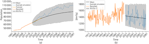
Example models of (a) population and (b) precipitation uncertainties. CI, confidence interval
Example models of (a) population and (b) precipitation uncertainties. CI, confidence interval
5 Strategies for resilience and their optimality
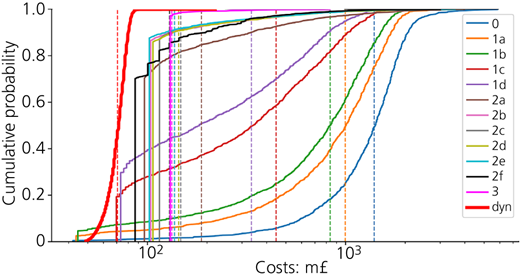
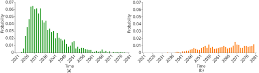
Once the future uncertainty with the key parameters is estimated, managers have to identify the different possible ways to ensure that they can continue to provide service, taking into consideration the many possible futures of what might happen. This step is a precursor to determining which of these interventions should be executed and in which order they can ensure the optimal level of resilience. For the example, the possible interventions are to reduce leakage by different amounts and to increase water supply by varying amounts. These are then combined into either static strategies – that is, it is decided now what is to be done over the investigated period, or dynamic strategies – that is, it is decided only what is to be presently done, and then, it is agreed that the situation will be reanalysed in the future using the same objective function. Once established, these strategies are analysed by running simulations of what may happen in the future. In the example, many different possible strategies were identified together with their total costs, in terms of reductions in service and interventions costs, using 1000 Monte Carlo simulations. A sample of the strategies used in the examples, the estimations of the costs and net benefit when compared to the reference strategy 0, and the cumulative distributions of the total costs are given in Tables 5 and 6 and Figure 3. Figure 4 shows the probabilities of executing interventions 2a and 3 in the investigated period when the dynamic strategy is followed. The probabilities of all other interventions are 0.
Investment strategies to ensure water supply resilience
| Label | Description | When | Time required |
|---|---|---|---|
| 0 | 0 | 0 | 0 |
| 1a | RL 2 Ml/d | 0 | 2 |
| 1b | RL 2.5 Ml/d | 0 | 2 |
| 1c | RL 6 Ml/d | 0 | 2 |
| 1d | RL 7 Ml/d | 0 | 2 |
| 2a | RWA 20 ML/d | 0 | 2 |
| 2b | RWA 40 ML/d | 0 | 2 |
| 2c | RWA 20 ML/d | 30 | 2 |
| 2d | RWA 40 ML/d | 50 | 2 |
| 2e | RWA 40; 20 ML/d | 0; 10 | 2; 2 |
| 2f | RWA 40; 10 10 ML/d | 10;15;30 | 2; 1; 1 |
| 3 | RWA 35 ML/d | 45 | 5 |
| Dynamic | Variable | ||
RL, reduce leakage; RWA, raise water availability
With respect to the static strategies, it can be seen that
Strategy 2f – that is, to raise the water availability by 40 ML/d at year 10, and then by 10 ML/d at year 15 and then again at 30, is the optimal strategy – that is, to yield the lowest average total costs/effects on service (132 m£). It has also a relatively high benefit–cost ratio. The selection of 2f would mean no investment now but investments are yet to come in year 15 and 30.
Strategy 3 and 2b, also have high net benefit, but lower benefit–cost ratios than 2f. The selection of strategy 3 or strategy 2b would mean investing 88 or 62 m over 60 years £. As not all of this money does not need to be committed now, it means our investment option would be to raise water availability by 20 ML/d in the next 5 years.
Strategy 1c – that is, to reduce leakage by 2 Ml/d immediately, will result in significantly higher total costs (429 m£) than in strategy 2f (297 m£).
The least uncertainty is associated with strategy 3, and the largest uncertainty is with strategy 0.
Strategy 0 could incur the lowest but could also incur the highest costs.
Net benefit of strategies
| Label | Results [m£] | |||||||
|---|---|---|---|---|---|---|---|---|
| [A] | [B] | [C] | [D] | [E] | [F] | [G] | [H] | |
| Base NPC over 60 years (mid) | Intervention costs over 60 years | NPC over 60 years (mid) [A] + [B] | Service risk | Total cost [C]+[D] | Benefit [D] of MS_0 −[D] of MS_x | B/C [E]/[C] | Net benefit [E] − [C] | |
| 0 | 42 | 0 | 42 | 1368 | 1410 | 0 | – | – |
| 1a | 42 | 2 | 44a | 923 | 967 | 444 | 10.2 | 401 |
| 1b | 42 | 3 | 45 | 780 | 824 | 588 | 13.2 | 543 |
| 1c | 42 | 28 | 70 | 359 | 429 | 1008 | 14.5 | 939 |
| 1d | 42 | 31 | 73 | 264 | 337 | 1104 | 15.1 | 1031 |
| 2a | 42 | 54 | 96 | 78 | 174 | 1290 | 13.4 | 1193 |
| 2b | 42 | 62 | 104 | 32 | 136 | 1335 | 12.9 | 1232 |
| 2c | 42 | 73 | 115 | 31 | 146 | 1337 | 11.6 | 1222 |
| 2d | 42 | 65 | 107 | 30 | 137 | 1337 | 12.5 | 1231 |
| 2e | 42 | 60 | 102 | 37 | 140 | 1330 | 13.0 | 1228 |
| 2f | 42 | 45 | 87 | 45 | 132 | 1323 | 15.3 | 1236 |
| 3 | 42 | 88 | 130 | 3 | 133 | 1364 | 10.5 | 1234 |
| dyn | 42 | 28 | 70 | 0.05 | 70 | 1368 | 19.4 | 1297 |
The best values of the static strategies are outlined in red in the table
Bold values are the dynamic strategy (which are better than any static strategy)
dyn, dynamic; NPC, net present cost
It can also be seen, however, that the dynamic strategy provides the lowest average total costs, 70 m£ (in terms of the overall sum between the intervention costs and monetarised reduction in service) – that is, it provides the optimal balance between resilience enhancement and intervention costs. It is also more certain than 0 but less than 3.
Here, it is also interesting to note the difference between using static and dynamic strategies in evaluating investment options. If static strategies are used in the example, no investment is currently required as 2f, the optimal strategy only requires raising the water availability by 40 ML/d in year 10 (i.e. lowest cost, 132 m£, and highest net benefit, 1234 m£). This is predominantly due to the reduction in the costs of inadequate service as it reduces the probability of not being able to meet demand to almost 0, and the costs of the staggered investments are discounted. If, however, another intervention strategy would be chosen (e.g. 2b), which is very close in total net benefit to 2f, a large investment would be required now.
If a dynamic strategy is used in the example, it is clear that no investment is currently required, and that intervention 2a will happen relatively early over the investigated period and intervention 3 relatively late (Figure 4). Of course, these decisions will need to be made at some point of time in the future. Considering that most managers do not seriously commit themselves to financing for 60 years ahead of time, the use of dynamic strategies provides a more accurate picture of reality through the consideration of management flexibility and leads to improved investment decisions.
6 Understanding cost drivers
In an uncertain environment, aside from the estimation of expected costs, with or without sensitivity analyses, managers need to have an idea on what is likely to contribute to these costs and who will bear them and why. This type of information needs to be generated in every strategy. Examples for three static strategies and the dynamic strategy are shown in Figures 5 and 6. Additionally, the uncertainty associated with the costs can be shown. The probability density function (pdfs) and cumulative distribution function (cdfs) for the total costs of strategies 0, 1c and 2b, and dynamic total costs are shown in Figures 7 and 8.
These graphs provide significant insight into the cost drivers and the stakeholders who must bear these costs, as well as why and when. For example, it can be seen for strategy 0 that a large percentage of the total costs (1390 m£, with a confidence interval for the 1000 simulations that ranges between 129 and 3266 m£) are due to the high environmental cost of pumping water beyond the critical intake level, but that the cost of fish not passing and the cost of unmet demand contributes significantly. The intervention costs, which are only due to routine maintenance over time, are relatively small in comparison. It can, however, also be seen that both strategies 1c and 2f significantly reduce these environmental costs but have increased intervention costs, due to the cost of leakage reduction and the costs of reservoir expansion.
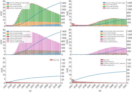
Costs associated with (a) strategy 0: total costs, costs of inadequate service and intervention costs and (b) strategy 1c: total costs, costs of inadequate service and intervention costs. PCC, per capital consumption
Costs associated with (a) strategy 0: total costs, costs of inadequate service and intervention costs and (b) strategy 1c: total costs, costs of inadequate service and intervention costs. PCC, per capital consumption
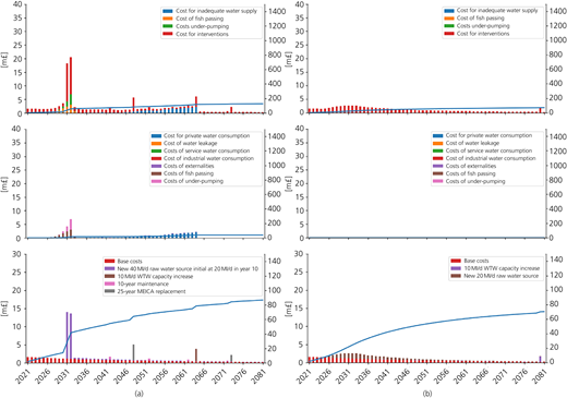
Costs associated with (a) strategy 2f: total costs, costs of inadequate service and intervention costs and (b) the dynamic strategy: total costs, cost for inadequate service and cost for interventions. MEICA, mechanical, electrical, instrumentation, control and automation assets; WTW, water treatment works
Costs associated with (a) strategy 2f: total costs, costs of inadequate service and intervention costs and (b) the dynamic strategy: total costs, cost for inadequate service and cost for interventions. MEICA, mechanical, electrical, instrumentation, control and automation assets; WTW, water treatment works
Figures 7 and 8 show the expected total costs – that is, the sum of the cost for inadequate service and the costs of intervention for over 60 years. Strategy 0 (Figures 7(a) and 7(b)) has mean expected total costs of 1390 m£, with a confidence interval that ranges between 129 and 3266 m£. Strategy 1c (Figures 7(c) and 7(d)) has mean expected total costs of 429 m£, with a confidence interval that ranges between 70 and 1514 m£. Strategy 2f (Figure 8(a)) has mean expected total costs of 132 m£, with a confidence interval that ranges between 87 and 1026 m£, while the dynamic strategy (Figure 8(b)) has the lowest mean expected total costs (70 m£).
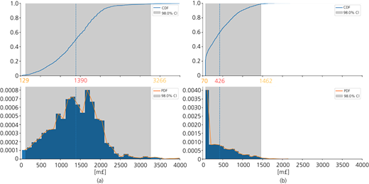
The (a) Cdf and Pdf for strategy 0 total costs and the (b) Cdf and Pdf for strategy 1c total costs. CI, confidence interval
The (a) Cdf and Pdf for strategy 0 total costs and the (b) Cdf and Pdf for strategy 1c total costs. CI, confidence interval
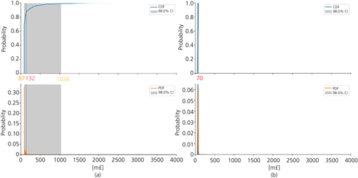
The (a) Cdf and Pdf for strategy 2f total costs and the (b) Cdf and Pdf for dynamic strategy total costs. CI, confidence interval
The (a) Cdf and Pdf for strategy 2f total costs and the (b) Cdf and Pdf for dynamic strategy total costs. CI, confidence interval
In addition to the costs, it is also possible to see why they are likely to be incurred and who will incur them. Examples are shown in Figure 9, which show the supply, demand, water level and the difference between supply and demand if strategy 0, 1c and 2f are followed. The supply-and-demand graphs show the amount of water available and required, as well as the 95% confidence intervals and the capacity of the water treatment works. The water level graphs show the mean water level in the reservoirs, the 95% confidence intervals, the highest possible water levels, the limit for fish passage and the water level required to avoid incurring environmental costs. The water supply–demand graphs show the mean of the water supply to cover the demand for all uses, as well as the 95% confidence intervals.
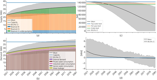
(a) Supply and (b) demand and (c) water level and (d) the difference between supply and demand if strategy 0 is followed
(a) Supply and (b) demand and (c) water level and (d) the difference between supply and demand if strategy 0 is followed
It can be seen in Figure 9(b) that the water demand is foreseen to increase over time, mainly due to the expected growth in domestic use and that the supply for it (Figure 9(a)) will lead to under-pumping of the reservoirs from which the water is drawn starting from year 2031. In Figure 9(d), it can also be seen that the average amount of water required to satisfy the demand is well above both the distribution capacity and the demand.
Figure 9(c) shows that under strategy 0, the water levels in the reservoirs are expected to be reduced below the critical level; that allows fish to pass by 2036 and below the level considered acceptable for environmental preservation. Figure 9(d) shows that the ratio between demand and supply is expected to turn negative (i.e. to cause a water shortage) by 2070.
With strategy 1c (Figure 10): (i) the expected need of under-pumping decreases significantly with respect to strategy 0, and it is not expected to start before year 2036; (ii) the point in time where the critical water levels are passed is postponed to the time interval between 2050 and 2060, and (iii) the ratio between demand and supply never becomes negative. With strategy 2f (Figure 11): (i) there is only likely to be a small amount of under-pumping before the construction of the new 10 Ml/d raw water source (i.e. year 10) and then none at all; (ii) the critical water level limits are never passed and (iii) the supply–demand ratio is always positive. A similar tendency can be seen with the dynamic strategy (Figure 12), as with strategy 2f. The differences, however, is that the interventions are only triggered when they yield the highest net benefit. The analysis associated with the dynamic strategy that there are only two types of interventions that may be triggered – that is, the construction of a new water source (intervention 3) and the increasing of the capacity of the existing water source by 20 Ml/day (intervention 2a). Intervention 3 might be triggered somewhere between 2041 and 2081 with a small probability. The probability is small because intervention 3 is only beneficial in the scenarios where there is a significant increase in demand, which has a small probability. Intervention 2a might be triggered in almost all the years, with a higher likelihood of being triggered earlier than later. This is because the net benefit of the investment is positive when there is only a small increase in demand.
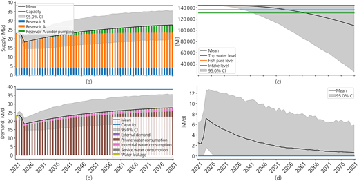
Supply (a) and demand (b) and water level (c) and the difference between supply and demand (c) if strategy 1c is followed
Supply (a) and demand (b) and water level (c) and the difference between supply and demand (c) if strategy 1c is followed
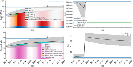
(a) Supply and (b) demand and (c) water level and (d) the difference between supply and demand if strategy 2f is followed
(a) Supply and (b) demand and (c) water level and (d) the difference between supply and demand if strategy 2f is followed
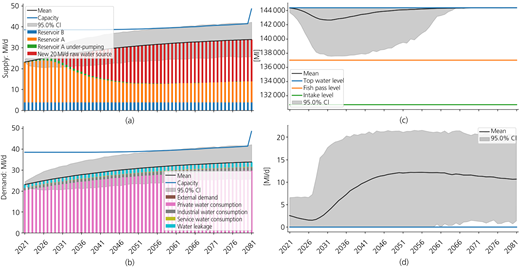
(a) Supply and (b) demand and (c) water level and (d) the difference between supply and demand if the dynamic strategy is followed
(a) Supply and (b) demand and (c) water level and (d) the difference between supply and demand if the dynamic strategy is followed
7 Conclusion
This paper demonstrates how to make investment decisions that optimally improve water supply resilience, taking into consideration both future uncertainty and management flexibility. It does so by appraising investment options using quantifiable benefits over time, including risk for multiple stakeholders. It is shown that this can be done with and without considering explicitly the ability of the manager to make decisions in the future based on new information. Considering management flexibility, however, provides more clarity as to whether an investment should be made or not, and if so, which intervention should be made and why.
For the example, it is shown that
If static strategies are used in the appraisal of project investment options, no investment is currently required. This is because strategy 2f, that is, raising the water availability by 40 ML/d at year 10, and then of 10 ML/d each time at years 15 and 30, is the optimal one, providing both the lowest expected total cost (i.e. 132 m£) and the highest expected net benefit (i.e. 1234 m£). This is principally due to the reduction in the costs of inadequate service, since when the water availability is expanded to 60 Ml/d over time, any chance that the water supply cannot satisfy the demand of one or more of the services, is small. Additionally, when this is done in three steps, the cost of interventions is pushed into the future, and is, therefore reduced through discounting. There is, however, a non-negligible probability that another intervention strategy would be chosen, for example, 2b, which is very close in total net benefit to 2f, which would mean that a large investment would be required now.
If a dynamic strategy is used in the appraisal, it is clear that no investment is currently required. It is likely that intervention 2a, that is, raising the water availability by 20 Ml/d, will happen relatively early over the investigated time period and intervention 3, that is, raising the water availability by 35 Ml/d, relatively late, but these decisions will need to be made at some point of time in the future which better reflects reality.
Acknowledgements
The authors would like to thank Scottish Water for their partial financing of this work and the technical support provided by Alan Scott in the creation of the example.
