Climate Change, Bank Fragility, and Systemic Risk Open Access

Climate change is one of the most pressing issues of our time.¹ Physical climate change, such as severe storms, more frequent floods, and catastrophic wildfires, disrupts firms’ businesses and operations. Some firms are adversely affected by climate regulations and transition policies. The crucial impacts of climate change generate attention to corporate managers, governments, and economists. On this point, central banks and international institutions also have expressed concerns that climate change can imperil financial stability and could cause next financial turmoil.²

Climate change, undoubtedly, can be a source of systemic risk.³ It is intuitive that climate change can generate cascading damage to the financial markets and institutions. A group of recent research shows that climate-related shocks can generate both micro- and macro-prudential risks (e.g., Battiston et al. (2021) and Brunetti et al. (2021)). According to the Bank of International Settlements (BIS), climate change could trigger the next financial crisis by exacerbating financial vulnerabilities (e.g., Bolton et al. (2020)). Previous studies have well documented that the interconnectedness in financial markets could easily amplify the detrimental impacts of climate change (e.g., Battiston et al., 2017; Stolbova et al., 2018). Motivated by these studies and the dramatic impacts of climate change, this paper examines how both physical and transitional climate changes lead to increases in systemic risk.

This analysis begins by examining the relationship between climate change and bank fragility. The baseline results show a positive relationship between climate change and systemic risk. In terms of economic significance, a one standard deviation increase in physical climate change exposure leads to about a 4.03% increase in systemic risk. The impact of transitional climate change is stronger. A one standard deviation increase in the environmental and climate policy uncertainty leads to about a 28.8% increase in systemic risk. The results indicate that climate change exacerbates bank fragility. In the next step, potential channels through which climate change impacts bank fragility are explored; the test results show that the impacts of climate change are more pronounced for banks with higher climate change exposure, higher loan synchronicity, and higher bank default probability.

Further, endogeneity concerns are addressed using the instrumental variable approach. A proper instrumental variable carries a significant relationship with climate change and affects systemic risk only through this channel.⁴ Two instruments are employed:the percentage of buildings in a flood zone and climate change concern (the estimated percentage of adults who believe global warming is already harming people in the U.S. now or within 10 years). The coefficients of instrumented variables are consistent with the baseline results, meaning that the relationship between climate change and systemic risk remains significantly positive under the instrumental variable specification.

Lastly, we investigate whether climate adaptation policy can build resilience to climate change. By exploiting the climate change adaptation plans across U.S. states, we analyze whether the climate adaptation policy can help mitigate the impacts of climate change. The test results show a significantly negative coefficient of the interaction term between climate change and adaptation policy. The results imply that climate adaptation can shield banks from the detrimental impacts of climate change, which in turn contributes to financial stability. Overall, the findings indicate that systemic risk with a climate adaptation policy differs from systemic risk without a climate adaptation policy.

This paper contributes to several strands of literature. First, this paper adds to the climate finance and sustainability literature. Previous studies document that it is important to understand the impact of climate change on corporate policies and financial markets (e.g., Gillingham et al., 2018; Vismara, 2019; Henderson and Serafim, 2020; Hong et al., 2020). Recent studies show that climate change is a new source of uncertainty, and it has potentially serious economic consequences (e.g., Barnett et al., 2020; Bolton and Kacperczyk, 2021; Engle et al., 2020; Giglio et al., 2021; Hong et al., 2020). Many studies provide empirical evidence that climate change poses large aggregate uncertainties to the economy and the financial system (Bolton and Kacperczyk, 2021; Choi et al., 2020; Painter, 2020; Sautner et al., 2023). This paper adds to that literature, providing evidence that climate change significantly affects systemic risk.

This study adds to the broader debate on the nature of systemic risk and its determinants. Previous literature finds that systemic risk is affected by bank size (e.g., Rochet and Tirole, 1996; De Jonghe, 2010; Leaven et al., 2016), by asset price bubbles (e.g., Brunnermeier et al., 2020), and by geographic diversification (e.g., Chu et al., 2020). Our study is also related to recent studies on financial networks (e.g., Acemoglu et al., 2015; Brunetti et al., 2019). In addition to these studies, we provide evidence that climate change increases systemic risk.

Our paper also contributes to a growing literature on the impact of sea level rise exposure. Several recent studies investigate the impact of sea level rise on residential property values (e.g., Baldauf et al., 2020; Murfin and Spiegel, 2020; Nguyen et al., 2020). This study is also related to the literature on disaster experiences and risk attitudes (e.g., Bharath and Cho, 2021). In line with this literature, this paper provides supportive evidence that sea level rise exposure has a negative impact on financial stability.

The remainder of the paper is organized as follows. Section 2 describes the data and sample statistics. Section 3 presents the main empirical results. In Section 4, the impact of climate adaptation actions is tested. In Section 5, we provide a conclusion.

The bank accounting data are obtained from the Commercial Bank Reports of Income and Condition (Call Reports) quarterly. The Call Reports contain banks’ balance sheets, income statements, and other information. The data on market capitalization and stock returns is collected from the Center for Research on Security Prices (CRSP). By focusing on banks, we do not include investment banks, investment management companies, and brokers. The list of all banks is obtained from the Federal Reserve Bank of New York’s Federal Reserve Banks link.⁵ The entire sample consists of 1,301 bank holding companies and commercial banks. The sample period runs from 1990 to 2016.

The main systemic risk measures are MES (marginal expected shortfall) and ΔCoVaR (the change in conditional value at risk).MES, constructed by Acharya et al. (2017), estimates how individual institutions’ stock returns react to the entire market. It assesses each financial institution’s exposure to systemic risk by measuring the average loss of market equity of an individual institution when the market return is in a lower tail. MES is defined as:

where R_i,_t is bank i’s stock return on day t, and R_m,_t is the market return on day t. The MES is calculated using the 5% worst days of market returns over the previous quarter of return data using the following equation:

where R_i,t represents the daily returns of an institution, and t to t^* represent the days on which the market is in the tail of its return distribution.

The next measure for systemic risk is ΔCoVaR, introduced by Adrian and Brunnermier (2016).ΔCoVaR represents the change in the value at risk (VaR) of the entire financial system that occurs when one institution falls into a state of distress. Whereas MES measures banks’ exposure to systemic risk,ΔCoVaR estimates the additional value at risk of the entire financial system that is associated with the experiencing distress (Chu et al., 2020). We calculate CoVa

where q is the q^th quantile of the return distribution. We set q as equal to 0.05, as same as Adrian and Brunnermier (2016). Following Adrian and Brunnermier (2016), the vector of state variables, M, is the change in the three-month Treasury yield, the change in the slope of the yield curve, the short-term TED spread, the change in the credit spread between Baa-rated bonds and the treasury rate, the weekly U.S. market returns, and the VIX index of stock market volatility. For each institution, we calculate ΔCoVaR as:

CoVaR measures the marginal contribution of an institution to overall systemic risk. One of the advantages of this measure is that the variation of ΔCoVaR comes entirely from the tail dependence, instead of from the time variation of state variables.

To proxy physical climate change, sea level rise exposure (hereafter Sea level rise) and the number of climate disaster by each state and year (hereafter Climate disaster ) are employed. The data for Sea level rise is obtained from the National Oceanic and Atmospheric Administration (NOAA). Sea level rise is set according to NOAA’s sea level rise “intermediate” scenario in the year 2040. The NOAA provides detailed geographical shapefiles that describe the latitudes and longitudes that would be inundated following an increase in average sea level compared with the year 2000. We match the sea level rise exposure at the city-level to be consistent with bank locations. To do this, the city-level data is obtained from the Urban Adaptation Assessment (UAA).⁶ UAA provides an interactive database led by the Notre Dame Global Adaptation Initiative (ND-GAIN). The data encompass over 270 cities within the U.S. including all 50 states whose populations are above 100,000.

The data for Climate disaster is obtained from the Federal Emergency Management Agency (FEMA).⁷ The data we use for Climate disaster is the number of climate disasters by state and year. FEMA provides the data for 61,344 disaster declaration cases since 1953 including flood, severe storms, hurricanes, fire, snow, drought, and tornado by each state and year (see Figure O1 in the Online Appendix). Figure O1 shows the cumulated number of climate disasters from 1984. We count and summarize the disaster declarations data by each state and year. Figure O1 documents that a large number of disasters declarations are caused by severe storms, hurricanes, and floods.

Proxy transitional climate change, we use Environmental and climate policy uncertainty and Firm-level environmental risk. The data for Environmental and climate policy uncertainty is obtained from the indices constructed by Noailly et al. (2022).⁸ The indices analyze 15 million news articles extracted from the archives of ten U.S. newspapers.⁹ They use machine learning techniques to build the database. 80,045 news articles on environmental and climate policy have been identified by using a supervised support vector machine algorithm. The indices scale the monthly counts of environmental and climate policy articles by the total monthly volume of news articles in order to represent the share of articles about environmental policy across ten large newspapers.

The data for Firm-level environmental risk is constructed by Hassan et al. (2019). ¹⁰ They adopt a machine learning keyword algorithm to produce a set of environmental policy bigrams and identify firm-level exposure. They employ a set of training libraries Z = {P₁, . . . ,P_Z}. Each containing the complete set of bigrams occurring in discussion of a particular topic. Topic-specific measures are used to identify risks associated with specific political topics.

Their firm-level environmental policy exposure measure is employed to proxy Firm-level environmental risk.

Table 1 presents the summary statistics of the main variables used in this paper. In our sample, the average of MES is 0.047121 and the standard deviation is 0.030846. The average of ΔCoVaR is 0.012098 and the standard deviation is 0.008249. The average of climate disaster (raw number) is 46, indicating that there are 46 instances of climate disaster declaration in each state and each year. The average of Environmental and climate policy uncertainty is 4.53034 and the standard deviation is 0.4235. The average of Firm-level environmental risk is 0.004109 and the standard deviation is 0.00399.

For the control variables, this study includes Ln(Assets), Ln(Asset)², Bank Capital, Profitability (ROA), Loan-to-Assets, Loan Growth, Loan Loss Provisions-to-Assets, Liquidity-to-Assets, Deposit-to-Assets, and Non-interest income-to-Assets. All of these control variables, which are common to the banking literature, are defined in Table O1 in the Online Appendix.

We start by running an ordinary least squares (OLS) regression to understand the relationship between climate change and systemic risk. To do so, we analyze the effect of climate change on systemic risk by estimating the following regression model:

where Systemic Risk _i,t+1Δ is measured by MES and CoVaR of bank i in quarter t + 1. β is the coefficient of interest that captures the change in a bank’s exposure to systemic risk in response to climate change. Climate change is divided into two categories: physical climate change and transitional climate change. To proxy physical climate change, we use Sea level rise, and alternatively, Climate disaster. To proxy transitional climate change, we use Environmental and climate policy uncertainty, and alternatively, Firm-level environmental risk.X_i,t denotes the bank-level control variables for bank i in quarter t. We include the bank-level fixed effects and quarter dummy variables to control for possible seasonality. Standard errors are clustered at the bank level to correct for potential cross- sectional and serial correlation in the error term (Petersen, 2009).

The baseline regression results are presented in Table 2. Panel A presents the estimation results using Sea level rise. Panel B presents the estimation results using Environmental and climate policy uncertainty. Across all the panels in Table 2, the results for four different regression specifications are presented. In columns (1) and (2), the dependent variable is MES, while in columns (3) and (4), the dependent variable is ΔCoVaR. In columns (1) and (3), we conduct multivariable regression including Ln(Assets), Ln(Asset)², Bank Capital, Profitability (ROA), Loan-to-Assets and Loan Growth. In columns (2) and (4), we add additional control variables such as Loan Loss Provisions-to-Assets, Liquidity-to-Assets, Deposit-to-Assets, and Non-interest income-to-Assets. If the coefficient ß to be significantly positive, it indicates that climate change leads to substantial systemic risk.

Overall, the results in Table 2 strongly support our empirical implication. Consistent with the hypothesis that climate change increases systemic risk, all the coefficients of climate change are significantly positive. This positive relationship is both statistically robust and economically meaningful. The coefficient of climate change in column (2) in Panel A is 0.0035, indicating that a one standard deviation increase in climate change leads to about 4.03% increase in systemic risk.¹¹ In Panel B, the coefficient of climate change in column (2) is 0.0210, indicating that a one standard deviation increase in the climate change leads to about 28.8% increase in systemic risk. These findings indicate that banks that are more vulnerable to climate change face higher levels of systemic risk.

Next, we conduct different sets of tests using alternative measures of climate change to ensure the baseline results. To proxy alternative physical climate change, we use Climate Disaster, and to proxy alternative transitional climate change, we use Firm-level environmental risk.Table 3 reports the test results for these measures. Same as Table 2, we include the bank fixed effects and time fixed effects. Standard errors are clustered at the bank level.

Consistent with the results in Table 2, the results in Table 3 support the implications that climate change induces systemic risk. All the coefficients of climate change are significantly positive. The positive relationships are both statistically robust and economically meaningful. The coefficient in column (2) in Panel A is 0.4627, indicating that a one standard deviation increases in climate change leads to about 1.69% increase in systemic risk. In Panel B column (2), the coefficient of Firm-level environmental risk is 1.0508, indicating that a one standard deviation increases in climate change leads to about 13.6% increase in systemic risk. Overall, the baseline results in Table 2 show that climate change increases systemic risk.

First, this study investigates how individual bank-level climate change exposure can explain the elevated contribution to systemic risk. Each bank has a different level of vulnerability to climate change conditions, therefore, climate change can affect bank-level fragility in disparate ways. Some banks incur costs from physical climate changes such as sea level rise or climate disasters, while other banks are more adversely affected by climate change related policies and regulations. Both physical climate events and costly climate transitions can cause financial systemic losses.

One challenge of bank-level climate change exposure is that it is difficult to quantify the climate exposure of individual bank level (Giglio et al., 2021). To address this point, we use firm-level climate change exposure data developed by Sautner et al. (2023).¹²Sautner et al. (2023) construct firm-level time-varying measures of climate change exposures using machine learning algorithms. They count the frequency of certain climate change bigrams in the transcript of earnings conference calls, then divide by the total number of bigrams in the transcript. Using this measure, which captures firm-level exposures related to both physical and transitional shocks associated with climate change, we estimate the following regression model to test the potential mechanism:

where Systemic Risk _i,tt+1 is measured by MES and ACoVaR of bank i in quarter t+1. Bank level exposrue _i,t is the bank-level climate change exposure level of firm i in quarter t.

Panel A of Table 4 reports the test results. In all regressions, we control for the time fixed effect and bank fixed effect. All standard errors are clustered by bank. In column (1), the dependent variable is MES. In column (2), the dependent variable is ΔCoVaR. In Panel A, climate change is proxied by sea level rise. Since climate and environmental risks are fundamentally downside risks for most firms (Seltzer et al., 2022), we expect to see a positive and significant coefficient of the interaction term between climate change and systemic risk.

The regression results are presented in Panel A. In column (1), the effect of bank-level climate change exposure on MES is positive and statistically significant. The coefficient is 5.2954 (t-stat = 1.84). The result on ΔCoVaR in column (2) is consistent. The coefficient of the interaction term is 1.1361 (t-stat = 2.30), which indicates that bank-level climate change exposure increases systemic risk. Overall, the results in Panel A of Table 4 suggest that bank-level exposure to climate change is an important driver for substantial change in systemic risk. These findings provide supporting evidence that banks that are more exposed to climate change contribute more to systemic risk.

Next, we investigate whether bank loan portfolio similarity exacerbates the impact of climate change on systemic risk. It is well documented in the literature that systemic risk tends to stem from interconnectedness and interlinkages among banks. Recent research finds that the interconnectedness across financial markets and institutions can easily amplify the effects of climate shocks through the indirect loss of asset values or self-reinforcing feedback loops (Battiston et al., 2017, 2021). For example, Allen et al. (2012) show that asset commonality can lead to spillover effects. Brunetti et al. (2019) show that correlation networks forecast financial crises. Goldstein et al. (2022) show that the correlation across financial institutions plays a major role in increasing their overall fragility. Moreover, it has been widely recognized that physical and transition risks are intertwined and represent a major source of systemic risk when they cause losses to levered financial intermediaries, generating financial instability on both an individual and systemic level (Battiston et al., 2016; 2021; Brunetti et al., 2021).

To test the possible mechanism, the following regression model is estimated:

In this regression specification, the interaction term picks up the differential effect of bank loan portfolio synchronicity. To proxy Bank loan synchronicity, we construct a measure capturing bank herding behaviors in lending.¹³ More specifically, this measure captures the tendency of banks to issue or close (sell) a given loan together in the same direction more often than would be expected if they issued or closed loans independently.

Panel B of Table 4 presents the estimation results. Column (1) reports the test result using MES, while column (2) reports the test results using ΔCoVaR. We expect the effect of climate change to be stronger for banks with higher loan synchronicity. In column (1) of Panel B, the coefficient of interaction term is significantly positive at 0.0121 (t-stat = 1.81), while in column (2) the coefficient of interaction term is 0.0034 (t-stat = 5.28). These positive associations are both statistically robust and economically meaningful. The results indicate that the effect of climate change on systemic risk is more pronounced for banks with higher loan synchronicity. Overall, the findings in Table 4 suggest that bank-level climate change exposure and bank loan portfolio similarity can potentially serve as channels through which climate change leads to substantial systemic risk.

Lastly, we investigate whether bank-level default risk explains the increased contribution to systemic risk. Banks’ assets are risky debt claims with capped upside, as a result, bad shocks to borrowers’ asset value can lead to a rise in banks’ asset volatility. Thus, climate-related shocks to bank asset value could potentially increase bank default risk. To proxy the bank-level default probability, the modified Merton model proposed by Nagel and Purnanandam (2020) is employed.¹⁴ This model takes into account the option-on-option nature of bank risk dynamics to ensure that the measure does not understate the default probability of banks. Using this measure, we estimate the following regression model to test the potential mechanism:

where Systemic Risk _i,t+1 is measured by MES and ΔCoVaR of bank i in quarter t +1. Bank default probability _{i t} is the bank-level default probability of bank i in quarter t.

Panel C of Table 4 reports the test results. In this panel, climate change is proxied by Environmental and climate policy uncertainty. In all regressions, we control for the time fixed effect and bank fixed effect. All standard errors are clustered by the bank, as was done in the baseline analyses. In column (1), the dependent variable is MES, while in column (2), the dependent variable is ΔCoVaR. In column (1), the effect of bank-level climate change exposure on MES is found to be significantly positive, with a coefficient of 0.0143 ( t-stat = 23.20). The result for ΔCoVaR in column (2) is consistent with this, with a coefficient of interaction term of 0.0009 (t-stat = 11.62). Overall, the results in Panel C suggest that bank-level default probability is an important driver for substantial change in systemic risk. Thus, the findings provide suggestive evidence that banks with higher default probability contribute more to systemic risk.

Climate change such as extreme weather events and/or transitions in policies and regulations are likely to be exogenous, thus the causal relation between climate change and systemic risk is not likely to be bidirectional. Nevertheless, in this section, we use instrumental variable analysis to address endogeneity concerns. A proper instrument is a variable that is significantly related to climate change and that affects systemic risk only through this channel.

The first instrument we use for Sea level rise is the percentage of building in flood zone in 2015. We obtained the data from an Urban Adaptation Assessment (UAA) report from Notre Dame University Global Adaptation Initiative. We present the two-stage least square regression results in Table 5. We predict that the instrumental variable (the percentage of building in flood zone in 2015 ) should be positively correlated with climate change. The first-stage regression results are consistent with this prediction, showing a coefficient of 0.00066 (t-stat = 30.21), which indicates that the instrumental variable is positively associated with the level of Sea level rise. Both the weak identification F-test and the over identification J-test pass the critical value of appropriate instrument. Next, we report the second-stage regression result using the predicted corruption from the first-stage regression in Panel A. The regression coefficient for MES is 0.3457 (t-stat = 2.72), while the coefficient for ACoVaR is 0.1444 (t-stat = 7.73), both of which are significantly positive. These results suggest that the coefficients of instrumented Sea level rise are consistent with our baseline results.

The second instrument we use for Environmental and climate policy uncertainty is climate change concern. Several groups of researchers recently discussed climate change concerns in relation to asset pricing (e.g., Engle et al., 2021; Pastor et al., 2021; Stroebel and Wurgler 2021). Climate change concern is the estimated percentage of adults who believe global warming is harming people in the U.S. either now or since 2014. The data is obtained from the UAA report from Notre Dame University Global Adaptation Initiative. The two-stage least square regression results are reported in Panel B of Table 5. We predict that the climate change concern should be positively correlated with climate change and find that the first-stage regression results are consistent with this prediction, that is, the coefficient is 1.0881 (t-stat = 2.73), indicating that the instrumental variable is positively associated with the level of Environmental and climate policy uncertainty. We then report the second-stage regression result using the predicted corruption from the firststage regression in the second and third columns in Panel B. The regression coefficient for MES is 0.0742 (t-stat = 2.02) and the coefficient for ΔCoVaR is 0.0333 (t-stat = 1.74), both of which are significantly positive. These results demonstrate that the coefficients of instrumented Environmental and climate policy uncertainty are consistent with our baseline results. Overall, then, the results in Table 5 suggest that the relationship between climate change and systemic risk remains significantly positive under the instrumental variable specification.

In this section, we explore whether climate change adaptation policy can mitigate the effects of climate change on systemic risk. To test this, we adopt the state-led climate change adaptation plans.¹⁵ The state-led climate change adaptation plans set out to prepare states for the impacts of climate change. It helps increase states’ resilience to the adverse effects of climate change. These climate change adaptation plans are rolled out in a staggered manner across states. As of March 2021, 19 states had finalized adaptation plans, and six states had adaptation plans underway (see the Online Appendix, Table O2). The climate adaptation plans include vulnerability assessments and actions to reduce the negative impacts of climate change or to take advantage of emerging opportunities. There are considerable variations in the content of climate adaptation depending on each state’ characteristics. For example, a climate adaptation plan in California is to focus on preventing wildfire and regulating carbon emission. In Florida, the adaptation plan is focused on protecting their lands from sea level rise.¹⁶

We analyze the effect of state-led climate change adaptation plans by estimating the following regression model:

where SystemicRisk_i,t+1Δis measured by MES and CoVaR of bank i in quarter t+1. β is the coefficient of interest that captures the change in banks’ exposure to systemic risk in response to climate change. Climate change is either Sea level rise or Firm-level environmental risk. Adaptation Plans_j,t is an indicator variable equal to one if the climate change adaptation plan is finalized in state j in quarter t and otherwise zero for others. X_i,t denotes the bank-level control variables. We include bank fixed effects and time fixed effects, and standard errors are clustered at the bank level.

We employ basically a difference-in-difference model. By applying this approach, the interaction term essentially captures how the systemic risk of banks with climate adaptation plans differs from the systemic risk of banks without climate adaptation plans. If climate adaptation mitigates the effect of climate change, banks that are facing high climate change should contribute less to systemic risk. By contrast, if climate change is merely a noisy shock, there should not be any differential response to the adoption of state-led climate change adaptation plans.

there should not be any differential response to the adoption of state-led climate change adaptation plans.

Table 6 reports the test results. In columns (1) and (2), we report the relationship between adaptation plans and climate change, while in columns (3) and (4), we present the results of the difference-in-difference analyses. The main finding in Panel A of Table 6 is that banks that face higher sea level rise and that operate within states that implement climate change adaptation plans contribute less to systemic risk. The coefficient of interaction term is negative and significant in column (4), indicating that adaptation plans reduce the effect of sea level rise. In Panel B, we find similar results. In Panel B column (3), the coefficient of interaction term is negative and significant, which suggests that climate adaptation actions can reduce the systemic risk caused by climate change. Overall, the results indicate that climate adaptation plans can shield banks from climate change and in doing so contribute to climate resilience.

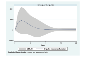
Furthermore, we take an in-depth look at how the relation between climate change and systemic risk evolves over time. One approach to investigate the relation is to estimate vector autoregression (VAR) at the aggregate level, and calculate an impulse response function (IRF). It quantifies how a shock to climate change affects future levels of systemic risk. We estimate VAR using 20 lags. The resulting IRF is reported in Figures 1 and 2. Figure 1 depicts IRF to quantify the effect of increasing sea level rise on aggregate systemic risk using a full sample. Figure 1 shows that a shock to sea level rise has a significant positive effect on systemic risk more than 10 quarters into the future. These results suggest that climate change can cause significant long-term fluctuations in systemic risk for at least up to two and half years.

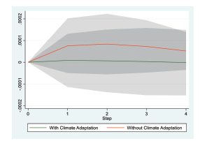
In Figure 2, we estimate separate VAR by aggregating firms in states with climate change adaptation plans (green line) and firms in states without adaptation plans (red line). The IRF in Figure 2 shows the effect of sea level rise on aggregate systemic risk on climate adaptation plans. In Figure 2, we find that the effect of climate change on systemic risk is more amplified for banks in states without climate adaptation plans. Banks without climate adaptation plans make a higher contribution to systemic risk. On the contrary, the contribution of systemic risk of banks with climate adaptation plans (green line) is almost flat, indicating that such banks make little contribution to systemic risk. Overall, the results in Figure 2 suggest that climate adaptation policies can help reduce the detrimental effects of climate change on systemic risk, which in turn contributes to financial stability.

Given that climate change can be a source of systemic risk, climate risk monitoring is one of the top priorities on the agenda of financial regulator and policy makers. Systemic risk has the potential to destabilize financial institutions and leads to serious negative consequences for financial markets and the broader economy. It is, thus, important to understand how climate change poses threats to financial markets. In line with these efforts, this paper provides evidence that climate change is the crucial driver of bank fragility and systemic risk. We find both physical and transitional climate changes exacerbate financial instability. Various climate change measures such as climate change news index, firm-level climate change exposure, and climate disasters show consistent results.

This study can be helpful for understanding the risks posed by climate change and its impact on financial stability. For instance, findings in this study provide supporting evidence that the impacts of climate change are more pronounced for banks with higher climate change exposure, higher loan synchronicity, and higher bank default probability. Equally, this study provides suggestive evidence that climate adaptation policies can reduce the detrimental impacts of climate change. Overall, the findings in this paper imply that climate adaptation policy can shield financial institutions and markets from negative impacts of climate change, contributing to climate resilience.

References

See, for example, Nordhaus (2019) and Giglio et al. (2021) and Hong et al. (2020).
For example, the European Central Bank published the first climate-related scenario analysis in January 2021, and the Bank of England followed shortly afterward in June 2021. Canada and France also began incorporating climate change analyses in their assessments. In September 2022, the Federal Reserve announced the start of a pilot project to assess the climate risk exposure of the six largest U.S. banks (Federal Reserve, 2022).
“Systemic risk” is the risk associated with the collapse or failure of a financial institution. The significant feature of systemic risk is that the risk from a broken-down financial institution spreads to relatively healthier institutions. The threats from climate change can be divided into two categories: physical and transitional risks. The physical climate risk is from climate events such as hurricanes or floods, which disrupt existing operations and impair the value of assets. Transitional climate risk is from new policies and regulations affecting current businesses and increasing adjustment costs.
Climate change could be exogenous to systemic risk. Nevertheless, we used instrumental variable analysis to address endogeneity concerns. A detailed discussion is in Section 3.3.
The focus on banks operating inside the U.S. ensures that all banks in the analysis are subject to a uniform bank regulatory regime.
The data can be downloaded via the following link: https://gain-uaa.nd.edu/?referrer=gain.nd.edu.
The data can be downloaded via the following link: https://www.fema.gov/about/openfema/data-sets.
We thank the authors for generously sharing their dataset.
The New York Times, Washington Post, Wall Street Journal, Houston Chronicle, Dallas Morning News, San Francisco Chronicle, Boston Herald, Tampa Bay Times, San Jose Mercury News, and San Diego Union Tribune.
The data can be downloaded via the following link: https://www.firmlevelrisk.com/links.
The difference could be calculated as 0.0035*0.355239/0.030846=4.03%.
The Georgetown Climate Center is tracking the implementation of these plans: https://www.georgetownclimate.org
Ray and Grannis (2015) identify nine sectors to categorize each plan: Agriculture, Biodiversity, Coasts/Oceans, Emergency Preparedness, Forestry, Infrastructure, Public Health, Water, and Other.