


Human capital has an inalienable nature, and the departure of key talents could make a firm's capital less profitable.
Our test exploits USA state courts’ staggered rejections of the inevitable disclosure doctrine (IDD), which improves the ability of key talent to switch jobs.
In a difference-in-differences setting, we find that relative to unaffected firms, firms experience a significantly increased stock price crash risk after the states where they are headquartered reject the IDD.
Overall, consistent with the view that a loss of key personnel can be an additional risk factor, our results suggest that an increased likelihood of key talent outflow can lead to the formation of bad news, which in turn results in stock price crashes.
1. Introduction
Investments in human capital are subject to considerable risk and are often associated with major managerial challenges (Levhari & Weiss, 1974). This is particularly true for investments on key talent. As a crucial component in a firm's assets, key talent is indispensable and irreplaceable. As Douglas Conant, a legendary business veteran, points out, talent management is the key to sustainable value creation. However, human capital has an inalienable nature, and it is difficult to retain the right talent and create systems that encourage talent to develop the right skills (Hart & Moore, 1994). For this reason, the loss of key talent may trigger abrupt stock price crashes (Israelsen & Yonker, 2017) [1].
A well-known example is the resignation of Apple's Chief Design Officer, Sir Jonathan Paul (“Jony”) Ive. Ive played a vital role in creating Apple's most recognizable products (i.e. the iPod, iPhone, iPad and MacBook) and is one of the world's most esteemed industrial designers. He is also known as Steve Jobs' “spiritual partner”. After nearly 30 years at Apple, Ive left the company in June 2019 to form his own independent design firm. His unexpected departure was widely viewed as “mark[ing] the end of an era for Apple” (CNN Business, June 28, 2019) and drove the firm value by $8bn [2].
The above anecdotal evidence is consistent with the argument that the actual departure of key talents can lead to a short-term stock price crash. However, it is less clear whether the likelihood of key talents' departure can trigger stock price crash in the relatively long-run. Specifically, does an increased likelihood of key talent outflow increase subsequent stock price crash risk? To answer this question, we use staggered rejections of the inevitable disclosure doctrine (IDD) as exogenous shocks to the likelihood of key talent outflow.
The IDD is a legal doctrine that can have the effect of preventing employees from accepting similar employment in the same field, or of limiting their responsibilities in the new firm, due to their high probability of revealing trade secrets (Godfrey, 2004). Rejection of the IDD (IDDR) occurs when a state court rules that the doctrine is not enforceable in the state. By rejecting the doctrine, the state removes an important mobility restriction on employees who provide a firm with valuable and sometimes irreplaceable human capital, thus increasing the likelihood of key talent outflow (Schutz, 2017; Flowers, 2018; Na, 2020) [3]. Since 1999, a total of 14 states in the USA with high concentrations of key talent (including California, Massachusetts and Washington) have rejected the IDD (Flammer & Kacperczyk, 2019). Importantly, the IDDR is a legal judgment made purely from a knowledge spillover perspective and is not associated with firm fundamentals or macroeconomic conditions. To verify this premise, we estimate a state-level hazard model on the likelihood of rejecting the IDD and find that this event is not triggered by ex ante average crash risk, local economic conditions or political factors. In other words, the staggered rejections of the IDD in these 14 states offer plausibly positive and exogenous shocks to key talent mobility. These plausibly exogenous events can help us identify the causal relation between the likelihood of key talent outflow and stock price crash risk.
We conjecture that the IDDR results in an increase in the subsequent stock price crash risk. The intuitions are as follows. As summarized by Chang, Chen, and Zolotoy (2017), three factors can affect stock price crash risk: (1) the likelihood of bad news formation, (2) the extent of managerial bad news hoarding and (3) the strength of the market response when bad news is revealed. IDDR improves key talent mobility, making it easier for key individuals in a firm to switch jobs. An increased likelihood of losing key talent can be an additional risk factor (Eisfeldt & Papanikolaou, 2013) that raise potential costs associated with the loss of organizational capital (including performance deterioration in the product market or increased financial distress risk) or the exposure of trade secrets to rival firms, which can result in a potentially adverse effect on investors' assessment of the firm's production efficiency and growth prospects. Due to increased labor mobility, the IDDR can also increase the likelihood of revealing negative internal information (managers misusing skilled labor, giving preference to bad projects for private benefits, etc.) that is otherwise concealable. Therefore, the IDDR can increase the likelihood of bad news formation through either giving rise to additional bad news or revealing existing bad news. Driven by career concerns, firm managers have strong incentives to strategically hoarding such bad news, gambling that it will ultimately be offset by subsequent good news (e.g. Bleck & Liu, 2007; Hutton, Marcus, & Tehranian, 2009; Benmelech, Kandel, & Veronesi, 2010; Kim, Li, & Zhang, 2011; Chang et al., 2017; Baginski, Campbell, Hinson, & Koo, 2018; Li & Zhan, 2019) [4]. Hidden negative information accumulates and eventually reaches a critical point where managers can no longer withhold it anymore, and the information is then revealed all at once, leading to a sudden stock price crash [5]. In addition, according to Jin and Myers (2006), if the news is sufficiently bad (e.g. the adverse effect of losing key talents is too high), managers can exercise an abandonment option and the bad news comes out even without hoarding, leading to a stock price crash [6].
Alternatively, a contrasting view could hold. As IDD rejections can not only reduce information asymmetries between firms and outsiders by making trade secrets more likely to be publicly available but also enable focal firms to hire key talents from competing firms and enhance their product market performances, such legal changes tend to reduce future stock price crash risk. Therefore, how IDDR affects stock price crash risk is eventually an empirical question.
We apply a difference-in-differences (DiD) analysis to a sample of 65,489 firm-year observations from 1990 to 2017. We find that IDDR is significantly associated with an increased stock price crash risk, proxied by negative skewness (NCSKEW). Specifically, after a state rejects the IDD, firms headquartered there experience a 0.077 increase in crash risk (t-statistic = 3.08). This result is also economically large, considering that the sample mean of NCSKEW is −0.018.
We conjecture that IDDR increases the potential costs associated with the loss of organizational capital (i.e. the departure of key talent), thus increasing the likelihood of bad news formation. Indeed, we document that IDDR dampens firms' fundamentals and increases their distress risk, suggesting that an increased likelihood of key talent outflow is associated with performance deterioration and, if disclosed, will be regarded as bad news by outside investors.
These results might seem a bit puzzling since some existing empirical evidence shows that policies aiming at protecting trade secret may result in higher information asymmetry and lower reporting quality (Li, Lin, & Zhang, 2018; Kim, Su, Wang, and Wu, 2021; Li & Li, 2020; Li & Jian, 2020; Hu & Lee, 2020) [7]. Therefore, at the first glimpse, the rejection of IDDs may reduce stock price crash risk. However, our results could hold because the adoption and the rejection of IDDs can affect stock price crash risk through different channels. It is possible that on a certain level of bad news, IDD adoption could induce managerial information hoarding and increase stock price crash risk [8]. A rejection event, however, could give rise to additional bad news, as indicated by Eisfeldt and Papanikolaou (2013) who argue that a loss of key personnel can be an additional risk factor. According to Jin and Myers (2006), if the news is sufficiently bad (e.g. the increased risk of losing key talents is too high), managers can exercise an abandonment option and the bad news comes out even without hoarding, leading to a stock price crash. Therefore, the dominating effect of IDD rejection events could be different.
To further support our argument, we examine two auxiliary predictions. First, we argue that rejecting the IDD should generate a stronger impact on crash risk for firms facing more competition. In industries with more competition, key individuals in firms have more outside options and thus are more likely to leave their jobs after IDDR, potentially a larger price crash. We measure industry competition using industry fluidity (Hoberg, Phillips, & Prabhala, 2014) and industry concentration (Herfindahl–Hirschman Index) and find supporting evidence consistent with our conjecture.
Our paper highlights the importance of stakeholder management, in particular, retaining key talent, on sustainable value creation. To support this new perspective, we demonstrate that the risk of key talent outflow is an important external determinant of stock price crash risk [9]. Our findings suggest that policies purely based on labor market conditions and trade secret protection can have unintended consequences in destabilizing stock price at the firm level. In this sense, our findings call for attention not only from financial regulators but also state legislators and human resources managers. In addition, as our findings highlight the formation of bad news associated with performance deterioration and distress risk, our findings complement prior studies that identify distress risk as a root of bad news and crucially determine stock price crash risk (Ni & Zhu, 2016; Jia, 2018; Andreou, Andreou, & Lambertides, 2021; John, Ni, & Zhang, 2025; Ni, Si, & Zhang, 2026) [10].
The rest of the paper is organized as follows. Section 2 summarizes institutional details related to rejections of the IDD and develops our main hypothesis. Section 3 describes our sample construction and empirical design. Section 4 presents our main results. Section 5 reports the results from extensive robustness tests. Section 6 provides discussion and conclusion of the paper.
2. Institutional background and hypothesis development
2.1 Institutional background
The IDD is designed to protect corporate trade secrets. A trade secret is a valuable but invisible intellectual property of a company that derives independent economic value from not being publicly known. Examples of trade secrets include formulas, practices, designs, patterns, instruments, etc. Generally speaking, trade secret owners have the right to prevent others from misappropriating or using their trade secrets. The U.S. Chamber of Commerce reports that publicly traded USA companies own an estimated $5 trillion worth of trade secrets [11]. Trade secrets are protected under state laws; every state in the USA offers some form of trade secret protection (Merges, Menell, & Lemley, 2003). The IDD is one such protection.
Unlike other trade secret protection laws, the IDD is a tool for granting injunctions on competition in the absence of actual misappropriation (Godfrey, 2004). It is motivated by the prospect of trade secret leaks arising from key talent outflow. Employers argue that even without actual misappropriation, the departure of employees with knowledge of trade secrets would, in many situations, lead to unavoidable disclosure or use of the trade secrets by competitors. When raised by an employer, such situations are carefully evaluated by a state court under the IDD. If a state court rules that the new employment would inevitably lead to the disclosure of a firm's trade secrets to competitors and cause the firm irreparable harm, the court can prevent the employee from taking the new employment or can limit the worker's responsibility in the new firm (Rowe, 2005). The doctrine was first applied to employees in technical fields, but its scope has expanded to employees with knowledge of any trade secret, including financial information and manufacturing, production and marketing strategies [12]. A total of 21 states have adopted the IDD.
Although the increased trade secret protection afforded by the IDD may be beneficial, many believe that the doctrine to be generally harmful, upsetting the balance between competition and labor mobility. First, “inevitable disclosure” is an undefined and misapplied term that can restrict competition, hamper freedom of contract and prevent employee mobility (Whaley, 1998). Potential application of the doctrine in lawsuits can also deter aspiring entrepreneurs from developing start-ups out of fear of being sued. This can inhibit venture funding opportunities and economic development (Brenner, 2001). Second, the doctrine has serious potential for abuse when used by employers as a litigation tactic for biding their time (Berkun, 2003). This is especially true in the technology industry, where time is essential. The employer can obtain a preliminary injunction or a temporary restraining order to prevent an employee with knowledge of a key technology from leaving for a competitor; while the litigation is pending, the employer can simply wait for market forces to make the relevant technology (and hence the litigation) obsolete, leaving the employee out of work and out of money.
In light of these serious issues, 14 states have rejected the IDD since 1999. IDDR occurs when a state court rules that the doctrine is not enforceable in the state. By rejecting the doctrine, a state removes an important mobility restriction on employees who provide a firm with valuable and sometimes irreplaceable human capital (Schutz, 2017; Flowers, 2018). California was among the first states to reject the IDD; one of the main reasons directly relates to the state's legal structure encouraging freedom of mobility for workers to move from established firms to start-ups (Gilson, 1999). Table 1 provides a list of the states that have rejected the IDD during our sample period, obtained from Flammer and Kacperczyk (2019). Several other studies have also explored how IDD rejections affect firm-level outcomes (Qiu & Wang, 2018; Patel & Devaraj, 2022; Cai, John, Ni, & Zhang, 2026).
Rejection of the inevitable disclosure doctrine (IDD) legislation
| State | Year | Case |
|---|---|---|
| AR | 2009 | Cellco Partnership v. Langston, No. 4:09CV00928 JMM (W.D. Ark. 2009) |
| CA | 2002 | Whyte v. Schlage Lock Co. , No. G028382 (Ct. of App. of California 2002) |
| FL | 2001 | Del Monte Fresh Produce Co. v. Dole Food Co. , Inc., 148 F. Supp. 2d 1322 (S.D. Fla. 2001) |
| GA | 2013 | Holton v. Physician Oncology Servs., LP, No. S13A0012, 2013 WL 1859294 (Ga. 2013) |
| MD | 2004 | LeJeune v. Coin Acceptors, Inc. , 381 Md. 288 (Md. 2004) |
| MA | 2012 | U.S. Elec. Servs. v. Schmidt, Civil Action No. 12–10845-DJC (U.S. Dist. CT. for the Dist. of Mass. 2012) |
| MI | 2002 | CMI Int'l, Inc. v. Intermet Int'l Corp. , 649 N.W.2d 808, 812 (Mich. Ct. App. 2002) |
| NH | 2010 | Allot Communications v. Cullen, 10-E−0016 (N.H. Merrimack Superior Ct. 2010) |
| NJ | 2012 | SCS Healthcare Marketing, LLC v. Allergan USA, Inc., N.J. Super. Unpub. LEXIS 2704 (N.J. Sup. Ct. Ch. Div. 2012) |
| NY | 2009 | American Airlines, Inc. v. Imhof, U.S. Dist. LEXIS 46750 (S.D.N.Y. 2009) |
| OH | 2008 | Hydrofarm, Inc. v. Orendorff, Ohio App. LEXIS 5717 (Ohio App. Ct. 2008) |
| VA | 1999 | Government Technology Services, Inc. v. Intellisys Technology Corp. , 51 Va. Cir. 55 (Va. Cir. Ct. 1999) |
| WA | 2012 | Amazon.com, Inc. v. Powers, Case No. C12-1911RAJ (W.D. Wash. 2012) |
| WI | 2009 | Clorox Co. v. SC Johnson & Son Inc. , 2:09-cv-00408-JPS (U.S. District Court, Eastern District of Wisconsin (2009) |
Note(s): This table summarizes rejection of the Inevitable Disclosure Doctrine (IDD)
2.2 Hypothesis development
IDDR is a legal judgment made purely from a knowledge spillover perspective and is not associated with firm fundamentals or macroeconomic conditions. Therefore, the staggered rejections of the IDD in these 14 states offer plausibly positive and exogenous shocks to the likelihood of key talent outflow. These events enable us to identify the causal relationship between the likelihood of key talent outflow and stock price crash risk in a difference-in-differences framework.
IDDR makes switching jobs easier for key talent. This represents a major managerial challenge, as the key individuals in a firm are invaluable and sometimes irreplaceable. Eisfeldt and Papanikolaou (2013) argue that human capital has risk characteristics distinct from those of physical capital, which is why firms are required to report “loss of key personnel” as an additional risk factor in their 10-K filings. In their framework, organizational capital is a durable input in production that is embodied in a firm's key talent. They argue that the departure of key talent causes not only a direct loss in firm value due to the loss of organizational capital but also indirect losses due to increased competition from rivals that now have inside knowledge of the firm's corporate practices. Therefore, increased key talent mobility can increase potential costs associated with the loss of organizational capital, including performance deterioration in the product market or even financial distress risks (Nguyen, Pham, & Qiu, 2023). These potential costs can, in turn, adversely affect investors' assessment of the firm's production efficiency and growth prospects. Also, increased key talent mobility increases the likelihood of revealing negative internal information (managers misusing skilled labor, giving preference to bad projects for private benefits, etc.) that is otherwise concealable, which further aggravates managerial career concerns (Li & Zhan, 2019). Therefore, we conjecture that IDDR can give rise to additional bad news or reveal existing bad news, inducing managers to strategically withhold or delay the disclosure of bad news due to career concerns (e.g. Bleck & Liu, 2007; Hutton et al., 2009; Benmelech et al., 2010; Kim et al., 2011; Chang et al., 2017; Baginski et al., 2018; Li & Zhan, 2019). Hidden negative information accumulates and eventually reaches a critical point where managers can no longer withhold it; the information is then revealed all at once, leading to a sudden stock price crash. Based on this intuition, we propose the following hypothesis.
Rejection of the IDD increases stock price crash risk.
A competing argument, however, is that IDDR can reduce stock price crash risk. By protecting trade secrets, IDD enforcement can increase information asymmetries between firms and outside investors (Callen, Fang, & Zhang, 2020; Kim et al., 2021). From this perspective, IDDR could reduce information asymmetries and potentially reduce future crash risk. Also, IDDR may improve labor market efficiency by facilitating the reallocation of human resources, benefiting firms in the affected states. In other words, one could argue that IDDR might improve firms’ human capital by making it easier for them to hire ideal employees from competitors, and therefore, firms' product market performances tend to be enhanced, and earnings manipulation will become less necessary (Li & Zhan, 2019). Based on this intuition, we propose the following competing hypothesis.
Rejection of the IDD decreases stock price crash risk.
3. Data and empirical design
3.1 Sample and variable construction
We start with all USA publicly listed firms in the Center for Research in Security Prices and Compustat from 1990 through 2017. This sample period is chosen because the CRSP-Compustat merged file achieves reasonably complete coverage of USA public firms starting in 1990, while Financial Accounting Standards Board (FASB)'s Accounting Standards Codification (ASC) 606 (Revenue Recognition) becomes effective in 2018 and materially changes the time-series properties of reported earnings. We exclude firms that are incorporated or headquartered outside of the USA Following the literature, we exclude financial firms and utility firms (SIC codes from 4,900 to 4,999 and from 6,000 to 6,999, respectively). Our main sample covers 65,489 firm-year observations.
We define the firm-specific weekly return for firm i at week j as , where is the residual from the following regression:
Here, denotes the weekly market return from week j and denotes the weekly return for firm i at week j. We use both the leads and the lags of the market returns to take account of nonsynchronous trading, following Scholes and Williams (1977) and Dimson (1979).
We adopt four different proxies to capture stock price crash risk. In our main results, following Chen, Hong, and Stein (2001), we use NCSKEW, computed as the ratio of the third moment of firm-specific weekly returns over the standard deviation of firm-specific weekly returns raised to the third power and then multiplied by −1:
where is the weekly return for firm i at week j and n is the total number of weeks in a fiscal year. A high NCSKEW indicates a high crash risk.
In robustness tests, we also consider three other proxies for stock price crash risk. Down-to-up volatility (DUVOL) is calculated as the natural logarithm of the standard deviation of weekly returns , during the weeks in which is lower than its annual means (“down” weeks) over the standard deviation of weekly returns during the weeks in which is higher than its annual means (“up” weeks). More specifically, DUVOL for each firm i at each fiscal year t is computed as
where is the number of “up” weeks and is the number of “down” weeks. A high DUVOL indicates a high crash risk.
The extreme sigma (ESIGMA) is the negative of the worst deviation of firm-specific weekly returns from the average firm-specific weekly return divided by the standard deviation of firm-specific weekly returns (Andreou, Louca, & Petrou, 2017). More specifically, for a given firm i in a fiscal year t, ESIGMA is defined as
where and are the mean and the standard deviation of the firm-specific weekly returns, respectively. A high ESIGMA indicates a high crash risk.
Finally, we define CRASHDUM as a dummy variable that equals one when firm i experiences at least one crash week during the fiscal year t and zero otherwise. A week is considered a crash week when the firm-specific weekly return is 3.2 standard deviations below the average firm-specific weekly return for the entire fiscal year (Kim et al., 2011) [13].
Other control variables include the following: (1) IDD, a dummy variable that equals one if the state where a firm is headquartered has adopted the IDD and zero otherwise; (2) lagged NCSKEW; (3) de-trended stock turnover ratio; (4) firm-specific stock return volatility; (5) past returns; (6) firm size; (7) market-to-book ratio; (8) leverage ratio; (9) return-on-assets and (10) accounting quality. Detailed descriptions of these variables can be found in Appendix Table A1. All continuous variables are winsorized at the 1st and 99th percentile. We report summary statistics of these variables in Table 2.
Summary statistics of main variables
| Num | Mean | Sd | P25 | Median | P75 | |
|---|---|---|---|---|---|---|
| (1) | (2) | (3) | (4) | (5) | (6) | |
| NCSKEWt+1 | 65,489 | −0.018 | 1.143 | −0.674 | −0.022 | 0.625 |
| IDDRt | 65,489 | 0.168 | 0.374 | 0.000 | 0.000 | 0.000 |
| IDDt | 65,489 | 0.560 | 0.496 | 0.000 | 1.000 | 1.000 |
| NCSKEWt | 65,489 | 0.002 | 1.062 | −0.641 | −0.026 | 0.595 |
| DTURNt | 65,489 | 0.002 | 0.085 | −0.025 | 0.000 | 0.027 |
| SIGMAt | 65,489 | 0.070 | 0.037 | 0.044 | 0.062 | 0.086 |
| RETt | 65,489 | −0.003 | 0.009 | −0.008 | −0.002 | 0.002 |
| SIZEt | 65,489 | 5.455 | 1.952 | 4.031 | 5.338 | 6.765 |
| MBt | 65,489 | 3.202 | 4.109 | 1.261 | 2.092 | 3.627 |
| LEVt | 65,489 | 0.193 | 0.186 | 0.014 | 0.157 | 0.315 |
| ROAt | 65,489 | −0.015 | 0.215 | −0.020 | 0.038 | 0.080 |
| ACCMt | 65,489 | 0.074 | 0.089 | 0.018 | 0.045 | 0.093 |
Note(s): This table reports summary statistics of variables used in the regressions estimated by the full sample consists of firm-year observations. Columns (1)-(6) report the summary statistics of the variables in the full sample. Variable definitions are provided in Table A1 in Appendix
Table 2 shows that about 17% of our sample is affected by IDDR. NCSKEW has a mean of −0.018 and a standard deviation of 1.143. In other words, the weekly return distributions are slightly positively skewed on average. These summary statistics are consistent with the results reported in existing studies.
3.2 Empirical design
The staggered rejections of the IDD in 14 USA states enable us to identify the causal relation between the likelihood of key talent outflow and stock price crash risk in a DiD framework. More specifically, we estimate the following panel regression:
where i indexes firm, s indexes the headquarter state, j indexes the region of the headquarter state and t indexes year [14]. is the NCSKEW for firm i located in state s in fiscal year t+1, and is a dummy variable that equals one if a firm's headquarter state s has rejected the IDD in year t and zero otherwise. The coefficient on , , is the one with main interest.
We include a vector of control variables () and firm-fixed effects (). In addition, following Acharya, Baghai, and Subramanian (2014), we control for regional time trends through the interaction of region dummies with year dummies (). These region-specific time trends enable us to non-parametrically account for time-varying differences in trade secret protection and in the IDDR across geographical regions (Acharya et al., 2014). We cluster standard errors at the headquarter state level to account for potential time-varying correlations in unobservable factors that affect different firms within the same headquartered state (Bertrand & Mullainathan, 2003; Bertrand, Duflo, & Mullainathan, 2004).
4. Main results
4.1 The determinants of rejection of the IDD
Before conducting our main tests, we want to verify the validity of using staggered rejections of the IDD as exogenous shocks to the likelihood of key talent outflow. Specifically, we examine whether the decision to reject the IDD may be driven by underlying political or economic conditions at the state level. For example, the IDDR might follow a period of high economic growth, and the negative impact on stock prices may merely reflect the mean reversion in economic activity and hence stock returns.
We estimate different Cox proportional hazard models where the “failure event” is the IDDR in a state. In other words, once a state rejects the IDD, it is dropped out of the sample. We consider an array of state-level political, economic and other prior observable factors, such as lagged average stock price crash risk, the adoption of the IDD, the lagged logarithm of gross domestic product (GDP) and GDP growth, the lagged state unemployment rate, the logarithm of total population, the union membership rate and the political balance (measured as the ratio of Democrat to Republican state representatives in the House of Representatives). We report the results in Table 3.
Determinants of the rejection of the IDD
| (1) | (2) | (3) | |
|---|---|---|---|
| State average NCSKEW | −0.062 | −0.385 | −0.317 |
| (0.242) | (0.641) | (0.584) | |
| State IDD | −0.295 | −0.299 | |
| (0.698) | (0.766) | ||
| State GDP Growth | −16.940 | −17.257 | |
| (13.462) | (13.753) | ||
| State log(GDP) | −0.265 | −0.701 | |
| (2.086) | (2.649) | ||
| State unemployment rate | −0.339 | −0.381 | |
| (0.219) | (0.236) | ||
| State log(population) | 1.617 | 2.113 | |
| (2.079) | (2.755) | ||
| State union membership rate | 0.033 | 0.024 | |
| (0.047) | (0.048) | ||
| State political balance | 0.164 | ||
| (0.161) | |||
| N | 1,060 | 1,060 | 1,012 |
| Adj_R2 | 0.000 | 0.158 | 0.154 |
Note(s): This table reports the results from a Cox proportional hazard model where the “failure event” is rejection of the Inevitable Disclosure Doctrine (IDD) in a state, i.e. once a state rejects the IDD, it drops from the sample. The sample period is from 1990 to 2017. All explanatory variables are lagged by one year. Robust standard errors clustered at the state level are reported in parentheses. Coefficients marked with *, **, and *** are significant at 10%, 5%, and 1%, respectively
Table 3 shows that the decision to reject the IDD is not a function of political, economic or other prior observable factors. This is consistent with existing studies suggesting that a court's issuance of a new precedent is likely to be at least in part unanticipated (e.g. Autor, 2003). In other words, Table 3 verifies that the staggered rejections of the IDD in these 14 states offer plausibly exogenous shocks to key talent mobility.
4.2 The rejection of the IDD and crash risk
To examine the causal relation between the likelihood of key talent outflow and stock price crash risk, we estimate panel regressions based on Equation (5) and report the results in Table 4.
Rejection of the IDD and stock price crash risk
| NCSKEWt+1 | ||||
|---|---|---|---|---|
| (1) | (2) | (3) | (4) | |
| IDDRt | 0.041** | 0.044** | 0.086*** | 0.077*** |
| (0.019) | (0.020) | (0.026) | (0.025) | |
| IDDt | 0.000 | −0.008 | ||
| (0.010) | (0.029) | |||
| NCSKEWt | 0.052*** | −0.054*** | ||
| (0.005) | (0.006) | |||
| DTURNt | 0.404*** | 0.384*** | ||
| (0.050) | (0.050) | |||
| SIGMAt | 0.694*** | −1.368*** | ||
| (0.163) | (0.199) | |||
| RETt | 14.723*** | 14.450*** | ||
| (0.542) | (0.542) | |||
| SIZEt | 0.056*** | 0.238*** | ||
| (0.004) | (0.011) | |||
| MBt | 0.018*** | 0.023*** | ||
| (0.001) | (0.001) | |||
| LEVt | −0.294*** | −0.430*** | ||
| (0.031) | (0.044) | |||
| ROAt | 0.120*** | 0.220*** | ||
| (0.031) | (0.041) | |||
| ACCMt | 0.313*** | 0.123*** | ||
| (0.042) | (0.042) | |||
| Firm FE | N | N | Y | Y |
| Region*Year FE | Y | Y | Y | Y |
| N | 65,489 | 65,489 | 65,489 | 65,489 |
| Adj_R2 | 0.011 | 0.035 | 0.023 | 0.055 |
Note(s): This table estimates rejection of the Inevitable Disclosure Doctrine (IDD) on stock price crash risk. All variables are as defined in Table A1 in Appendix. The sample period covers 1990 through 2017. Columns (1)-(2) control for region-times-year-fixed effects. Columns (3)-(4) control for firm-fixed effects and region-times-year-fixed effects. Robust standard errors are clustered at the state-of-headquarter level. Robust standard errors are reported in parentheses. Coefficients marked with *, **, and *** are significant at 10%, 5%, and 1%, respectively
Table 4 shows that IDDR is associated with an increase in the subsequent stock price crash risk. The coefficient on IDDR is significantly positive under all specifications. For example, in column (4), after controlling for both firm-fixed effects and region × year fixed effects, IDDR is associated with a 0.077 increase in NCSKEW in the subsequent year (t-statistic = 3.08). Considering that the mean NCSKEW is −0.018, this result is both statistically significant and economically large. Meanwhile, the adoption of the IDD (IDD) does not affect stock price crash risk.
Our DiD approach relies on the assumption that, before IDDR, the crash risks of affected and unaffected firms evolved in the same manner. To confirm that our analysis does not simply capture trends unrelated to the IDDR, we examine if there is a pre-event difference in crash risk between affected and unaffected firms in Table 5. Specifically, we re-run all the columns in Table 4 after replacing IDDR with five dummy variables: IDDR−2, IDDR−1, IDDR0, IDDR1 and IDDR2+. These variables indicate the years relative to the IDDR. For example, IDDR−2 indicates that it is two years before rejection of the IDD, IDDR1 indicates that it is one year after the IDDR and IDDR2+ indicates that it is at least two years after the IDDR. The other two variables are defined accordingly in a similar fashion.
Time tests around the rejection of the IDD
| NCSKEWt+1 | ||||
|---|---|---|---|---|
| (1) | (2) | (3) | (4) | |
| IDDR(−2)t | 0.013 | 0.013 | 0.039 | 0.034 |
| (0.043) | (0.041) | (0.045) | (0.038) | |
| IDDR(−1)t | −0.020 | −0.015 | −0.001 | 0.004 |
| (0.032) | (0.030) | (0.034) | (0.035) | |
| IDDR(0)t | 0.085** | 0.086** | 0.117*** | 0.110*** |
| (0.038) | (0.039) | (0.042) | (0.035) | |
| IDDR(+1)t | 0.016 | 0.024 | 0.032 | 0.039 |
| (0.036) | (0.037) | (0.037) | (0.039) | |
| IDDR(2+)t | 0.036** | 0.039* | 0.102*** | 0.087*** |
| (0.018) | (0.020) | (0.028) | (0.031) | |
| IDDt | −0.000 | −0.007 | ||
| (0.010) | (0.030) | |||
| NCSKEWt | 0.052*** | −0.054*** | ||
| (0.005) | (0.006) | |||
| DTURNt | 0.404*** | 0.385*** | ||
| (0.050) | (0.050) | |||
| SIGMAt | 0.691*** | −1.370*** | ||
| (0.162) | (0.199) | |||
| RETt | 14.717*** | 14.446*** | ||
| (0.537) | (0.540) | |||
| SIZEt | 0.056*** | 0.237*** | ||
| (0.004) | (0.011) | |||
| MBt | 0.018*** | 0.023*** | ||
| (0.001) | (0.001) | |||
| LEVt | −0.294*** | −0.429*** | ||
| (0.031) | (0.044) | |||
| ROAt | 0.120*** | 0.220*** | ||
| (0.031) | (0.041) | |||
| ACCMt | 0.314*** | 0.123*** | ||
| (0.042) | (0.042) | |||
| Firm FE | N | N | Y | Y |
| Region*Year FE | Y | Y | Y | Y |
| N | 65,489 | 65,489 | 65,489 | 65,489 |
| Adj_R2 | 0.011 | 0.035 | 0.023 | 0.055 |
Note(s): This table conducts timing tests around rejection of the Inevitable Disclosure Doctrine (IDD) on stock price crash risk. All variables are as defined in Table A1 in Appendix. The sample period covers 1990 through 2017. Columns (1)-(2) control for region-times-year-fixed effects. Columns (3)-(4) control for firm-fixed effects and region-times-year-fixed effects. Robust standard errors are clustered at the state-of-headquarter level. Robust standard errors are reported in parentheses. Coefficients marked with *, **, and *** are significant at 10%, 5%, and 1%, respectively
We focus on the regression coefficients from IDDR−2 and IDDR−1, as they indicate whether there is any difference between the affected and unaffected firms prior to the IDDR. All of the columns in Table 5 show that the parallel trend assumption is not violated, given that none of the coefficients on IDDR−2 or IDDR−1 are statistically significant or economically large. The impact of the IDDR starts to appear after the rejection: the coefficients on IDDR0 and IDDR2+ are both significant [15].
To provide additional evidence that IDDR can indeed increase the likelihood of bad news formation, in Table 6, we conduct some additional analyses. In column (1), we show that IDDR on average is associated with a 2% net human capital outflow, as proxied by the net hiring rate. The evidence in column (2) shows that this significant loss of human capital is accompanied by a sharp decline in subsequent sales growth, which may result from heightened business competition due to the loss of key talents. That is, IDDR dampens firms' competitive advantages to some extent.
Rejection of the IDD and firm-level outcomes
| NETHIREt | GSALEt | AZt | EDFt | |
|---|---|---|---|---|
| (1) | (2) | (3) | (4) | |
| IDDRt | −0.017* | −0.022** | −0.613* | 3.098* |
| (0.009) | (0.010) | (0.362) | (1.790) | |
| Controls | Y | Y | Y | Y |
| Firm FE | Y | Y | Y | Y |
| Region*Year FE | Y | Y | Y | Y |
| N | 78,615 | 80,750 | 73,926 | 70,758 |
| Adj_R2 | 0.179 | 0.206 | 0.603 | 0.479 |
Note(s): This table estimates rejection of the Inevitable Disclosure Doctrine (IDD) on firm-level outcomes. All variables are as defined in Table A1 in Appendix. The sample period covers 1990 through 2017. All columns control for firm-fixed effects and region-times-year-fixed effects. Robust standard errors are clustered at the state-of-headquarter level. Robust standard errors are reported in parentheses. Coefficients marked with *, **, and *** are significant at 10%, 5%, and 1%, respectively
We further examine whether an increased likelihood of key talent outflow results in severe performance deterioration, specifically increased financial distress risk. Following Fairhurst, Liu, and Ni (2020), we use two measures of distress risk. The first measure is AZ, the Altman's Z-score (Altman, 1968), a higher level of which indicates a lower likelihood of financial distress. The second measure, expected default frequency (EDF), is the EDF measure of Bharath and Shumway (2008), which is a simplified version of Merton's (1974) structural distance-to-default model. A higher level of EDF indicates a higher likelihood of default. Evidence in columns (3)-(4) shows that the overall financial health of affected firms deteriorates as well, as we observe a significant increase in distress risk [16]. Ni and Zhu (2016) indicate that firms with severe performance deterioration due to financial distress or high default risk are more likely to fail, leading to stock price crashes. Andreou et al. (2021) reveal a strong positive relation between distress risk and stock price crashes. Therefore, the results presented in this subsection establish that the likelihood of key talent outflow is an important determinant of stock price crash risk, and the influence tends to be exerted through affecting the formation of bad news [17].
4.3 Cross-sectional analyses
To further support our argument, we examine two auxiliary predictions. First, we argue that IDDR should generate a stronger impact on crash risk for firms facing more competition. In industries with more competition, key individuals in firms have more outside options and thus are more likely to leave their jobs after IDDR, potentially leading to a large price crash. We measure industry competition using industry fluidity (Hoberg et al., 2014) and industry concentration (Herfindahl–Hirschman Index). We divide our full sample equally into high and low industry competition subsamples based on these two measures. We re-run the regression in Equation (5) for both subsamples and report the results in Panel A of Table 7.
Cross-sectional analysis
| Panel A: Industry competition | ||||
|---|---|---|---|---|
| NCSKEWt+1 | ||||
| Fluid | HHI | |||
| (1) | (2) | (3) | (4) | |
| High | Low | Low | High | |
| IDDRt | 0.096** | 0.023 | 0.097** | 0.026 |
| (0.041) | (0.031) | (0.039) | (0.036) | |
| Controls | Y | Y | Y | Y |
| Firm FE | Y | Y | Y | Y |
| Region*Year FE | Y | Y | Y | Y |
| Difference test | 3.14* | 3.32* | ||
| (p-value) | (0.082) | (0.074) | ||
| N | 20,940 | 21,081 | 31,718 | 32,539 |
| Adj_R2 | 0.052 | 0.063 | 0.061 | 0.058 |
| Panel B: Reliance on key talents | ||||
|---|---|---|---|---|
| NCSKEWt+1 | ||||
| R & D intensity | SG & A intensity | |||
| (1) | (2) | (3) | (4) | |
| High | Low | High | Low | |
| IDDRt | 0.097** | 0.041 | 0.124*** | 0.016 |
| (0.039) | (0.027) | (0.034) | (0.030) | |
| Controls | Y | Y | Y | Y |
| Firm FE | Y | Y | Y | Y |
| Region*Year FE | Y | Y | Y | Y |
| Difference test | 4.22** | 10.03*** | ||
| (p-value) | (0.045) | (0.003) | ||
| N | 32,820 | 31,725 | 32,921 | 31,623 |
| Adj_R2 | 0.063 | 0.052 | 0.059 | 0.057 |
Note(s): SG & A: selling, general and administrative. This table examines the cross-sectional differences of rejection of the Inevitable Disclosure Doctrine (IDD) on stock price crash risk. All variables are as defined in Table A1 in Appendix. The sample period covers 1990 through 2017. All columns control for firm-fixed effects and region-times-year-fixed effects. Robust standard errors are clustered at the state-of-headquarter level. Robust standard errors are reported in parentheses. Coefficients marked with *, **, and *** are significant at 10%, 5%, and 1%, respectively
Panel A of Table 7 reports results consistent with our conjecture. Among firms in industries with high fluidity (i.e. high competition), IDDR is associated with a 0.096 increase in the crash risk (t-statistic = 2.34), while among firms in industries with low fluidity (i.e. low competition), IDDR is only associated with a 0.023 increase in crash risk (t-statistic = 0.74). Similar results are also obtained in subsamples divided by high and low industry concentration. Among firms in industries with a low Herfindahl-Hirschman Index (HHI) (high competition), IDDR is associated with a 0.097 increase in crash risk (t-statistic = 2.49), while among firms in industries with a high HHI (low competition), IDDR is only associated with a 0.026 increase in crash risk (t-statistic = 0.72).
Second, the risk of losing key talent should be more relevant to firms that rely heavily on key talent. We construct two proxies to measure firms' reliance on key talent. First, Hall (2002) suggests that firms with research and development (R&D) expenditure rely heavily on key talent, as at least 50% of R&D spending goes toward the wages and salaries of highly educated scientists and engineers. Second, Eisfeldt and Papanikolaou (2013) suggest that selling, general and administrative (SG&A) expenses directly capture a firm's organizational capital embodied in its key talent. Following these two studies, we use R&D spending and SG&A expenses (both divided by total assets) to proxy for firms' reliance on key talent. We divide our full sample equally into high- and low-key talent-reliance subsamples based on these two measures. We re-run the regression in Equation (5) for both subsamples and report the results in Panel B of Table 7.
Consistent with our conjecture, our main result primarily stems from firms that rely heavily on key talent. For example, among firms with high R&D spending (high SG&A expenses), IDDR increases crash risk by 0.097 (0.124) with a t-statistic of 2.49 (3.65). Meanwhile, among firms with low R&D spending (low SG&A expenses), IDDR only increases crash risk by 0.041 (0.016) with a t-statistic of 1.52 (0.53).
In summary, the results documented in this subsection further support our argument that the likelihood of key talent outflow is an important determinant of stock price crash risk, and the heterogeneity effects across firms are unneglectable. Importantly, the IDDR is intended to enhance labor market efficiency, while the unintended stock market crashes concentrate in sectors that are highly competitive and innovative. Therefore, policymakers need to pay more attention on firms operate under both high competitive pressures and high failure rates, of which the leave of key talents is more of a concern.
5. Robustness tests
5.1 Stack-cohort approach
Recent econometrics studies have noted that the two-way fixed effects estimator from staggered DiD events could be biased due to the use of already-treated units as controls (Baker, Larcker, & Wang, 2022). To address this issue, we treat each IDD rejection event as a cohort and then pool the data of treated and control firms across cohorts to estimate the average treatment effect. For each cohort, we retain observations in the 10-year (−5, +5) event window and created a sample consists of treated firms, i.e. firms that experience the IDD rejection in that year and “clean” control firms, i.e. firms that in states unaffected by the IDD rejections throughout the sample period. We then stack the cohorts together and construct a firm-year-cohort level sample. To be consistent with the baseline regressions, we control for cohort-times-firm- and cohort-times-region-times-year-fixed effects in the model. In Table 8, estimation results show that our baseline findings still hold, and the effects emerge only after the IDD rejection events occur, but not before, suggesting that the potential “bad control” problem do not bias our results much.
Stack-cohort approach
| NCSKEWt+1 | ||
|---|---|---|
| (1) | (2) | |
| IDDRt | 0.054** | |
| (0.023) | ||
| IDDR(−2)t | 0.022 | |
| (0.047) | ||
| IDDR(−1)t | 0.032 | |
| (0.049) | ||
| IDDR(0)t | 0.097* | |
| (0.054) | ||
| IDDR(+1)t | 0.050 | |
| (0.041) | ||
| IDDR(2+)t | 0.059* | |
| (0.033) | ||
| Cohort*Firm FE | Y | Y |
| Cohort*Region*Year FE | Y | Y |
| N | 90,219 | 90,219 |
| Adj_R2 | 0.087 | 0.087 |
Note(s): This table examines the effect of the rejection of the Inevitable Disclosure Doctrine (IDD) on stock price crash risk based on a stack-cohort approach. All variables are as defined in Table A1 in Appendix. The sample period covers 1990 through 2017. All columns control for cohort-times-firm- and cohort-times-region-times-year-fixed effects. Robust standard errors are clustered at the state-of-headquarter level. Robust standard errors are reported in parentheses. Coefficients marked with *, **, and *** are significant at 10%, 5%, and 1%, respectively
5.2 Propensity score matching
In our main results, we have used all available firms in the CRSP-Compustat universe with sufficient data to compute our variables. One potential concern is that significant variations in firm characteristics within the full sample could affect our regression results. To address this concern and show that our results are not driven by differences in fundamentals between affected and unaffected firms, we construct a propensity score-matched sample. Specifically, we follow the procedures in Serfling (2016) and begin by retaining all observations for affected and unaffected firms in the year prior to the IDDR. We then estimate the probability of being an affected firm by estimating a logistic regression, using the vector of control variables in the baseline model as well as industry-fixed effects. We match each affected firm in year t−1 to the control firm with the closest propensity score (without replacement). We report the results based on this propensity score-matched sample in Table 9.
Propensity score matching
| Panel A: Pre-match regression and post-match diagnostic regression | ||
|---|---|---|
| Pre-match | Post-match | |
| (1) | (2) | |
| IDD | −0.430*** | −0.001 |
| (0.056) | (0.083) | |
| NCSKEW | 0.050* | −0.011 |
| (0.029) | (0.043) | |
| DTURN | −0.798*** | 0.355 |
| (0.273) | (0.386) | |
| SIGMA | 4.886*** | 0.112 |
| (0.762) | (1.146) | |
| RET | −4.595 | 1.233 |
| (3.230) | (4.816) | |
| SIZE | 0.072*** | 0.005 |
| (0.017) | (0.025) | |
| MB | −0.009 | 0.001 |
| (0.007) | (0.010) | |
| LEV | −0.591*** | −0.241 |
| (0.171) | (0.252) | |
| ROA | −0.486*** | 0.068 |
| (0.116) | (0.179) | |
| ACCM | −0.020 | −0.049 |
| (0.309) | (0.470) | |
| Industry FE | Y | Y |
| N | 24,440 | 2,566 |
| Pseudo_R2 | 0.033 | 0.008 |
| Panel B: Post-match differences | ||||
|---|---|---|---|---|
| Treated | Control | Differences | T-value | |
| (N = 1,283) | (N = 1,283) | |||
| (1) | (2) | (3) | (4) | |
| IDD | 0.533 | 0.531 | 0.002 | 0.12 |
| NCSKEW | 0.056 | 0.074 | −0.018 | −0.41 |
| DTURN | −0.004 | −0.008 | 0.004 | 1.00 |
| SIGMA | 0.079 | 0.079 | 0.000 | −0.14 |
| RET | −0.003 | −0.003 | 0.000 | 0.48 |
| SIZE | 5.663 | 5.670 | −0.007 | −0.10 |
| MB | 3.193 | 3.185 | 0.008 | 0.05 |
| LEV | 0.165 | 0.170 | −0.006 | −0.77 |
| ROA | −0.051 | −0.057 | 0.006 | 0.60 |
| ACCM | 0.079 | 0.080 | −0.001 | −0.39 |
| Panel C: Estimation based on the propensity-score-matched sample | ||
|---|---|---|
| NCSKEWt+1 | ||
| (1) | (2) | |
| IDDRt | 0.066** | |
| (0.028) | ||
| IDDR(−2)t | 0.047 | |
| (0.029) | ||
| IDDR(−1)t | 0.035 | |
| (0.031) | ||
| IDDR(0)t | 0.081* | |
| (0.041) | ||
| IDDR(+1)t | 0.009 | |
| (0.029) | ||
| IDDR(2+)t | 0.115*** | |
| (0.038) | ||
| Controls | Y | Y |
| Firm FE | Y | Y |
| Region*Year FE | Y | Y |
| N | 28,517 | 28,517 |
| Adj_R2 | 0.055 | 0.055 |
Note(s): This table present statistics of post-match differences in propensity score matching. Panel A presents parameter estimates from the logistic model used to estimate propensity scores for firms in the treatment and control groups. In Panel B, Column (1) presents sample average of firm characteristics in the treated group; Column (2) presents sample average of firm characteristics in the control group; Column (3) presents the sample mean difference test between Columns (1) and (2); Column (4) presents the t-value of the sample mean difference test between Columns (1) and (2). Panel C reports estimation based on the propensity-score-matched sample. The regressions control for firm- and region-times-year-fixed effects. Robust standard errors are clustered at the state-of-headquarter level. Robust standard errors are reported in parentheses. Definitions of all these variables are provided in Table A1 in Appendix. Coefficients marked with *, **, and *** are significant at 10%, 5%, and 1%, respectively
Panels A and B of Table 9 show that our propensity score matching procedure successfully eliminates most of the variation in control variables. In other words, results from this propensity score-matched sample should not be driven by the differences in firm fundamentals between affected firms and their control firms. We re-run our main results using this propensity score-matched sample and confirm that our main results still hold.
5.3 Controlling for concurrent events
Our full sample covers the time period from 1990 to 2017. During this period, events other than IDDR could potentially affect crash risk. One such event is adoption of the IDD, which we have effectively controlled throughout the paper. In this subsection, we control for four other state-level concurrent events that might affect crash risk.
The first event is a 1999 ruling on shareholder legislation. The ruling, made by the Ninth Circuit Court of Appeals on July 2, 1999, makes it difficult for shareholders to engage in class actions in affected states (Chu, 2017). We define NINTH as a dummy variable that equals one if the state where a firm is headquartered is under the Ninth Circuit's jurisdiction and zero otherwise. POST is a dummy variable that equals one for year 1999 onwards and zero otherwise. NINTH_POST is the interaction term of NINTH and POST. In column (1) of Table 10, we control for NINTH_POST in Equation (5) (the individual items of NINTH and POST are absorbed by firm and year fixed effects, respectively), and our main result still holds.
Controlling for concurrent events
| NCSKEWt+1 | |||||
|---|---|---|---|---|---|
| (1) | (2) | (3) | (4) | (5) | |
| IDDRt | 0.071*** | 0.075*** | 0.077*** | 0.077*** | 0.070*** |
| (0.025) | (0.025) | (0.025) | (0.025) | (0.025) | |
| NINTH_POSTt | 0.027 | 0.027 | |||
| (0.029) | (0.029) | ||||
| WDLt | −0.330*** | −0.330*** | |||
| (0.058) | (0.058) | ||||
| RTWt | −0.104*** | −0.095*** | |||
| (0.013) | (0.015) | ||||
| ANTIt | 0.065* | 0.061* | |||
| (0.037) | (0.036) | ||||
| Controls | Y | Y | Y | Y | Y |
| Firm FE | Y | Y | Y | Y | Y |
| Region*Year FE | Y | Y | Y | Y | Y |
| N | 65,489 | 65,489 | 65,489 | 65,489 | 65,489 |
| Adj_R2 | 0.055 | 0.055 | 0.055 | 0.055 | 0.055 |
Note(s): This table estimates the rejection of the Inevitable Disclosure Doctrine (IDD) on stock price crash risk by controlling for concurrent events. All variables are as defined in Table A1 in Appendix. The sample period covers 1990 through 2017. All columns control for firm-fixed effects and region-times-year-fixed effects. Robust standard errors are clustered at the state-of-headquarter level. Robust standard errors are reported in parentheses. Coefficients marked with *, **, and *** are significant at 10%, 5%, and 1%, respectively
The second concurrent event we consider is the adoption of wrongful discharge laws. Wrongful discharge laws, which have largely arisen from common law, are a collective term describing limitations on an employer's discretion to terminate employees (Bird & Knopf, 2009; Acharya et al., 2014; Fairhurst et al., 2020). We define WDL as a dummy variable that equals one if the state where a firm is headquartered has adopted wrongful discharge laws and zero otherwise. Column (2) of Table 10 shows that the effect of IDDR is still strong after controlling for the adoption of wrongful discharge laws.
States with right-to-work laws do not allow union membership and the payment of union fees to be used as conditions of employment (John, Knyazeva, & Knyazeva, 2015). To examine whether the adoption of right-to-work laws affects our main result, we define RIGHT as a dummy variable that equals one if the state where a firm is headquartered has adopted right-to-work laws and zero otherwise. We include RIGHT in the regression in column (3) of Table 10 and still find a robust result for the IDDR.
The final concurrent event we consider is the adoption of anti-takeover laws. Anti-takeover laws are a set of regulations that prohibit or severely limit a company from acquiring another company, primarily in instances involving hostile takeovers [18]. In column (4) of Table 9, we define ANTI as a dummy variable that equals one if a firm's state of incorporation has adopted one of the five anti-takeover laws and zero otherwise. Our main result still holds after including this variable.
Finally, in column (5) of Table 10, we include all four concurrent events into our regression. Regression results suggest that our main finding is not driven by these potential concurrent events.
5.4 Placebo test
One might argue that our main result can be driven by chance. To show that this is not the case, we conduct placebo tests by randomizing both the assignment of affected states (with no replacement) and enactment years (chosen randomly from the sample period 1990–2017). Specifically, we estimate the effect of pseudo-events on pseudo-affected states with the full set of control variables in the baseline regression and store the coefficients and standard error estimates for each placebo test. We repeat this procedure 5,000 times and report the distribution of placebo coefficient estimates in Figure 1. The mean of placebo coefficient estimates is −0.0003, which has an opposite sign with the actual estimate from Table 4. The actual estimate for IDDR, 0.077, is larger than the placebo estimates in 96.6% (=4,832/5,000) of placebo samples, implying that the probability of randomly observing the actual estimate when the null effect of the IDDR is in fact true is smaller than 5%. These results indicate that our baseline findings are unlikely to be driven by chance.
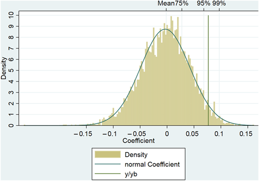
Distribution of placebo coefficient estimates. This figure shows the result from placebo tests by randomizing both the assignment of treated states (with no replacement) and enactment years (chosen randomly from the sample period 1990–2017). In particular, we estimate the effect of pseudo-events on pseudo treated states with the full set of control variables in the baseline regression and store the coefficients and standard error estimates for each placebo test. We repeat this procedure for 5,000 times. The vertical line shows the actual coefficient from our baseline regression
Distribution of placebo coefficient estimates. This figure shows the result from placebo tests by randomizing both the assignment of treated states (with no replacement) and enactment years (chosen randomly from the sample period 1990–2017). In particular, we estimate the effect of pseudo-events on pseudo treated states with the full set of control variables in the baseline regression and store the coefficients and standard error estimates for each placebo test. We repeat this procedure for 5,000 times. The vertical line shows the actual coefficient from our baseline regression
5.5 Alternative empirical specifications
We conduct various robustness checks to show that our main results are not driven by a particular empirical specification. Table 11 summarizes the results. First, we consider four alternative proxies for crash: NCSKEWt+2, DUVOL, the ESIGMA and a crash dummy (CRASHDUM). We repeat the analysis in Table 4 by replacing NCSKEWt+1 with one of the four alternative proxies. We find qualitatively similar results using these alternative proxies for crash risk.
Additional robustness checks
| Panel A: Alternative measures of crash risk | ||||
|---|---|---|---|---|
| NCSKEWt+2 | DUVOLt+1 | ESIGMAt+1 | CRASHDUMt+1 | |
| (1) | (2) | (3) | (4) | |
| IDDRt | 0.057** | 0.049* | 0.048*** | 0.014* |
| (0.024) | (0.027) | (0.015) | (0.009) | |
| Controls | Y | Y | Y | Y |
| Firm FE | Y | Y | Y | Y |
| Region*Year FE | Y | Y | Y | Y |
| N | 59,969 | 64,490 | 64,550 | 64,556 |
| Adj_R2 | 0.037 | 0.064 | 0.066 | 0.045 |
| Panel B: Alternative model specifications | ||||
|---|---|---|---|---|
| NCSKEWt+1 | ||||
| Two-way cluster | Sic2*year FE | Excluding delaware firms | Excluding current-year firms | |
| (1) | (2) | (3) | (4) | |
| IDDRt | 0.077*** | 0.077*** | 0.072** | 0.077*** |
| (0.025) | (0.027) | (0.028) | (0.024) | |
| Controls | Y | Y | Y | Y |
| Firm FE | Y | Y | Y | Y |
| Region*Year FE | Y | Y | Y | Y |
| N | 65,489 | 24,474 | 63,179 | 63,223 |
| Adj_R2 | 0.055 | 0.052 | 0.055 | 0.055 |
| Panel C: Specific subsamples | ||||
|---|---|---|---|---|
| NCSKEWt+1 | ||||
| −0.5≤Sales growth≤1 | Manufacturing firms | Excluding 2008–2009 observations | 1995–2015 | |
| (1) | (2) | (3) | (4) | |
| IDDRt | 0.060** | 0.139*** | 0.078*** | 0.075*** |
| (0.023) | (0.029) | (0.028) | (0.027) | |
| Controls | Y | Y | Y | Y |
| Firm FE | Y | Y | Y | Y |
| Region*Year FE | Y | Y | Y | Y |
| N | 60,629 | 31,971 | 60,201 | 50,556 |
| Adj_R2 | 0.054 | 0.059 | 0.059 | 0.054 |
| Panel D: Firm location issues | ||||
|---|---|---|---|---|
| NCSKEWt+1 | ||||
| State firms≥20 | Excluding geographical disperse industries | Adjusted headquarter | Excluding headquarter-movers | |
| (1) | (2) | (3) | (4) | |
| IDDRt | 0.077*** | 0.091*** | 0.067*** | 0.075*** |
| (0.024) | (0.027) | (0.024) | (0.024) | |
| Controls | Y | Y | Y | Y |
| Firm FE | Y | Y | Y | Y |
| Region*Year FE | Y | Y | Y | Y |
| N | 63,223 | 61,478 | 65,489 | 59,637 |
| Adj _R2 | 0.055 | 0.056 | 0.055 | 0.056 |
Note(s): This table examines the robustness of rejection of the Inevitable Disclosure Doctrine (IDD) on stock price crash risk through conducting additional tests. All variables are as defined in Table A1 in Appendix. The sample period covers 1990 through 2017 except for special indication. All columns control for firm-fixed effects and region-times-year-fixed effects except for special indication. Robust standard errors are clustered at the state-of-headquarter level. Robust standard errors are reported in parentheses. Coefficients marked with *, ** and *** are significant at 10%, 5% and 1%, respectively
Second, we examine if alternative model specifications affect our results. We consider the following alternative specifications: (1) double-cluster standard error by headquarter states and year; (2) control for industry × year fixed effects in addition to region × year fixed effects; (3) exclude firms incorporated in Delaware to avoid potential tax shelter benefits and (4) regard IDD rejection year as transition years and exclude observations in those years. Our results are robust across all of these alternative model specifications.
Third, we examine whether our results are driven by a particular subsample. We consider the following conditions: (1) include only firms with total sales growth rates of between −50% and 100%; (2) include only manufacturing firms; (3) exclude the financial crisis period (2008–2009) and (4) include only the 1995–2015 subsample. We find similar results in these subsamples.
Finally, given that our results depend on information about the locations of firm headquarters, we conduct additional exercises to see if our results are sensitive to location issues. We consider the following conditions: (1) include only states with at least 20 headquartered firms; (2) exclude firms operating in industries with a geographically dispersed workforce to alleviate the concern that workers may be located outside the state of headquarters (Agrawal & Matsa, 2013); (3) use the updated information rather than the information provided by Compustat on headquarter states [19] and (4) exclude firms that have changed their headquarters throughout our sample period. We find similar results based on these conditions.
6. Discussion and conclusion
A business cannot succeed without key individuals behind the wheel. However, unlike managing physical assets, managing key talent is a form of art. Without a clear strategic plan, talent management can disintegrate just as quickly as any other organizational process that lacks clear direction, especially when facing threats from an increasingly competitive and transparent labor market. With many businesses disregarding this crucial part of success, the wrong approach could be costly, resulting in stock price crashes.
In this paper, we support this view by exploiting the staggered rejections of the IDD as positive and exogenous shocks to the likelihood of key talent outflow. We provide evidence of a causal relationship between the likelihood of key talent outflow and stock price crash risk, especially for firms that face more industry competition and rely more heavily on key talent.
Our study has important policy and managerial implications. First, our results suggest that policies aimed at improving labor market efficiency can have unintended consequences for stock price stability at the firm level. In this sense, our findings should be relevant to not only financial regulators but also state legislators, as both parties have an interest in protecting financial stability. Second, when facing a competitive labor market with high mobility, managers need to spend extra effort to retain key talent. This is especially true for firms that rely heavily on key talent or operate in highly competitive industries. Given the growing embrace of competitive labor markets, freedom of contract and employee mobility, talent management needs to keep up with the trends for sustainable value creation.
Our research could throw light on future studies. In particular, our empirical specification is based on USA listed firms. An interesting and important research question is whether the lift of human capital mobility restrictions could have similar effects on Chinese listed firms. China provides an attractive out-of-sample laboratory. In China, mobility restrictions due to the “inevitable” disclosure of trade secrets are not as strong as in the USA and do not exhibit geographic variations. The Labor Contract Law (2008, amended 2013) only provides some general guidance on this issue. Therefore, any positive shock to key talent departure risk is likely to be of lower intensity for Chinese listed firms. Offsetting this, daily price limits and less-developed short-selling mechanisms could make the incorporation of bad news into stock prices slower, which may exaggerate future stock price crashes. Taken together, it is ex ante ambiguous whether the effect of enhancing the risk of losing key talents on stock price crash risk would be stronger or weaker for Chinese listed firms, and we leave it for future research.
Notes
“Loss of key personnel” is an important risk factor that needs to be reported under Item 1A in 10-K filings. For example, in 2019, Apple reported that “Much of the Company's future success depends on the continued availability and service of key personnel, including its Chief Executive Officer, executive team and other highly skilled employees” (page 12). The annual report identified the high demand and the intense competition for experienced personnel in the technology industry as major threats for loss of key personnel.
“What Jony Ive's Departure Means for Apple's Stock” (https://fortune.com/2019/06/28/jony-ive-leaving-apple-stock/)
In Section 2.1, we provide additional institutional background and discuss the legal considerations for rejecting the IDD.
Prior studies indicate that the disclosure of bad news may lead to reduced executive compensation or job termination (e.g. Verrecchia, 2001; Graham, Harvey, & Rajgopal, 2005; Kothari, Shu, & Wysocki, 2009).
In the example of Ive leaving Apple, since the announcement, both Bloomberg and The Wall Street Journal have reported that Ive had become disengaged with Apple for years. Despite this long-term disengagement, most of the design team members were unaware of Ive's departure until the announcement day. The announcement also caught the markets by surprise. For detailed reports, please refer to “Inside Apple's Long Goodbye to Design Chief Jony Ive” (by Mark Gurman from Bloomberg, June 28th, 2019) and “Jony Ive Is Leaving Apple, but His Departure Started Long Ago” (by Tripp Mickle from The Wall Street Journal, June 30th, 2019).
In the framework of Jin and Myers (2006), the amount of bad news that insiders are willing to absorb is limited. Thus, insiders must take one of the two actions: (1) If a sufficiently long run of bad firm-specific news is encountered, insiders exercise an abandonment option and all of the bad news comes out at once, and abandonment means a stock price crash, or (2) if a mild negative news is encountered, insiders can hoard the news by making up the difference between the firm's actual performance and investors' estimate of that performance.
It is worth noticing that the evidence of the influence of IDD adoption on firms' information environment is actually mixed. Gao, Zhang, and Zhang (2018) document a significant decrease in upward earnings management after IDD adoption. Li and Li (2020) show that management earnings forecast frequency and forecast horizon increases after IDD adoption. By comparison, Callen et al. (2020) show that IDD adoption increases firms’ financial reporting opacity. In addition, Li et al. (2018) and Kim et al. (2021) report that firms respond to their states’ recognition of the IDD by reducing disclosure and withholding more information. The evidence presented by Gao et al. (2018) and Li and Li (2020) may imply that IDD adoption is associated with a reduction in crash risk, while the latter three results may predict the opposite.
Li and Jian (2020) show that the adoption of IDD increases stock price crash risk. However, this result concentrates in the year of adoption and disappears in the next year following the adoption of IDD. Therefore, although the adoption of IDD seems could increase stock price crash risk, this effect is at most mild and temporary, possibly due to the complex information-related changes.
Other external determinants include liquidity (Chen et al., 2001; Chang et al., 2017), religiosity (Callen & Fang, 2015a), short selling (Callen & Fang, 2015b; Ni & Zhu, 2016; Deng, Gao, & Kim, 2020), accounting policy (DeFond, Hung, Li, & Li, 2015), analyst coverage (Kim, Lu, & Yu, 2019), product market threats (Li & Zhan, 2019) and internal controls (Lobo, Wang, Yu, & Zhao, 2020)
In the framework of Jin and Myers (2006), the formation of bad news is at least as important as subsequent bad news hoarding. They indicate that crash risk does not depend just on opaqueness: Two firms that are equally opaque can have different crash risk if one has more firm-specific risk or if abandonment is more costly for one firm than the other.
“The Case for Enhanced Protection of Trade Secrets in the Trans-Pacific Partnership Agreement”, available at: https://www.amcham.or.id/images/amcham_updates/TPP%20Trade%20Secrets%20Study%208-19-13.pdf.
PepsiCo, Inc. v. Redmond, 54 F.3d 1262, United States Court of Appeals, Seventh Circuit, May 11th, 1995.
The value of 3.2 is chosen to generate a frequency of 0.1% in the normal distribution.
We follow the traditional classification and classify the U.S. states into 6 regions: (1) New England (CT, MA, ME, NH, RI and Vermont); (2) Mid-Atlantic (DC, DE, MD, NJ, NY and PA); (3) Midwest (IA, IL, IN, KS, MI, MN, MO, ND, NE, OH, SD and WI); (4) West (CA, CO, ID, MT, NV, OR, UT, WA and WY); (5) South (AL, AR, FL, GA, KY, LA, MS, NC, SC, TN, VA and WV) and (6) Southwest (AZ, NM, OK and TX).
As the baseline DID result captures average treatment effect, it does not imply that crash risk of treated firms in every post-event year is higher than before. The timing test suggests that in the year of IDD rejection, stock prices of treated firms drop for a large scale due to the increased risk of human capital outflow. In the next year of IDD rejection, it is likely that stock prices do not drop that much relative to the pre-periods due to mean-reverting issues, and therefore, the obtained coefficient on IDDR(+1) is insignificant. For subsequent years, the stock price crash becomes prominent again after the mean-reverting effect diminishes.
Because expected default frequency (EDF) is usually very small to facilitate interpretation of the estimation results, we multiply the original value of EDF by 1,000.
In un-tabulated results, we conduct a path analysis and find that the increase in financial distress risk could partially explain the relation between rejection of the IDD and stock price crash risk.
Anti-takeover laws include control share acquisition laws, director duty laws, business combination laws, poison pill laws and fair price laws (Karpoff & Wittry, 2018).
As Compustat only provides information on the most recent state of headquarters, we retrieve information on the historical state of incorporation from this link: https://sraf.nd.edu/data/, which compiles relevant data based on firms' SEC electronic filings since 1994. For years before 1994, we use the information available for each firm in Compustat.
The supplementary material for this article can be found online.

