Dynamic determinants of price volatility across energy commodities: crude oil, natural gas, coal, and uranium markets

The global energy landscape continues to be shaped by traditional energy carriers such as crude oil, natural gas, coal, and increasingly uranium used for nuclear power. These commodities are often described as the “lifeblood of the industrial economy” because they play a central role in global production and energy security (Esen and Bayrak, 2017). Fluctuations in these markets reverberate far beyond the sectors that directly consume these fuels. They influence real-world economic activity, alter inflationary dynamics, and shape the behaviour of financial markets, including commodity futures, equity indices, and currency exchange rates. These interconnections mean that a sudden rise in oil prices, for example, can tighten liquidity, raise borrowing costs, shift investment flows, and ultimately affect trade balances and geopolitical relations between producing and consuming nations (Wang et al., 2020; Aladwani, 2025a).

A central question in empirical energy economics is the extent to which macroeconomic fundamentals, such as GDP growth, interest rates, industrial output, and commodity-specific demand and supply shocks, drive energy price volatility. Fama's (1970) Efficient Market Hypothesis (EMH) offers a theoretical lens: in a semi-strong efficient market, all publicly available information, including macroeconomic data, is already reflected in current prices, leaving little scope for systematic forecasting. Consequently, many studies on energy futures have concluded that these markets exhibit weak-form inefficiencies, implying that past price movements alone have limited predictive power (Tabak and Cajueiro, 2007). However, the EMH specifically addresses price-based predictability and does not preclude the possibility that external, observable fundamentals influence the underlying drivers of price volatility, even if they are not explicitly embedded in past price patterns.

Empirical work employing multifractal detrended fluctuation analysis on Brent and WTI crude oil series (Tabak and Cajueiro, 2007) demonstrates that price dynamics exhibit multifractal properties across varying economic conditions. These findings highlight that energy markets possess long-range correlations and scaling behaviours that cannot be captured by simple random walk models. However, as the study primarily tests weak-form market efficiency, it does not directly assess whether macroeconomic variables or structural factors influence the observed volatility. The rationale is that, while price series may efficiently reflect all previously observed information, they can still mechanically respond to new macroeconomic events that alter risk perceptions, supply and demand equilibria, and market participants' risk-adjusted discount rates.

For example, tightening monetary policy can increase the cost of capital, reduce investment in new energy capacity and potentially amplify cyclical volatility. Similarly, significant supply disruptions arising from geopolitical tensions in oil-producing regions can introduce volatility induced by shocks that is not captured by past price behaviour alone.

Therefore, the next step is to operationalise these macroeconomic drivers within a rigorous econometric framework, fit the models to high-frequency energy price data, and conduct out-of-sample predictive tests to evaluate the added explanatory power of macroeconomic variables. If macroeconomic fundamentals prove to be significant predictors of energy price volatility, this would challenge the conventional view derived from the EMH that energy markets are effectively blind to fundamental shocks. It would also open the door to more nuanced trading strategies and risk management approaches that exploit these systematic links. In summary, classical tests of weak-form efficiency emphasise the unpredictability of energy futures based on past prices; however, they do not fully rule out the influence of observable macroeconomic and structural factors on volatility dynamics. Accordingly, this study moves beyond price only predictability tests and focuses on the structural aspects that may systematically affect energy price fluctuations and persistence.

Building on this motivation, the central question guiding the study is as follows: which economic, financial, geopolitical, and uncertainty-related factors determine energy market volatility, and how do these determinants shape observed movements in energy prices?

A multivariate GARCH-MIDAS model was employed to address the central question of the study, incorporating a comprehensive set of variables used to forecast volatility across energy sources. Although this model includes many variables, it also introduces numerous parameters, which can reduce estimation efficiency and increase the risk of overfitting. To mitigate this complexity, the adaptive LASSO technique proposed by Zou (2006) is combined with the log-likelihood function. In line with Maranzano et al. (2023), a subset of “Beta weighting” parameters is held constant during estimation to avoid identification problems. Finally, the Generalized Information Criterion (GIC), as suggested by Atkinson (1980) and expanded by Fan and Tang (2013), is used to identify the optimal tuning parameter for the adaptive LASSO method. Two main reasons make this approach attractive: firstly, the multivariate GARCH-MIDAS model delivers superior predictive power compared with the standard GARCH-MIDAS model. Second, its variable selection capability allows for the identification of the most influential variables affecting energy price volatility.

Volatility of energy sources has been a subject of sustained investigation by scholars and practitioners alike. This research seeks to identify the primary determinants of such volatility and enhance predictive model precision. Grasping the drivers behind energy market fluctuations is essential for several stakeholders. First, when energy prices swing widely, policymakers confront significant concerns regarding energy security and economic stability. Second, institutional investors exploit market volatility to manage risk. The valuation and hedging of commodity derivatives are closely connected to energy futures movements, and sophisticated volatility management can improve returns while mitigating risk by capitalising on price variability. Third, accurate volatility forecasts contribute to macroeconomic models' robustness, thereby informing better policy decisions and economic planning. Fourth, uranium, a critical input for nuclear power generation, is experiencing renewed attention amid the global pivot towards low-carbon energy sources, yet its price remains exceptionally volatile due to a range of influencing factors. Despite its strategic importance, uranium has received less academic attention than other energy commodities, such as natural gas or crude oil. Therefore, this study addresses this research gap by examining the political, economic, and market-driven factors that underlie uranium price volatility.

The findings indicate that the main determinants of crude oil price volatility are default-yield spread, financial market uncertainty, geopolitical risk uncertainty, and macroeconomic uncertainty. Similarly, default-yield spread, financial market uncertainty, and macroeconomic uncertainty are the principal drivers of natural gas price volatility. In addition, coal price volatility is primarily affected by demand and supply within the coal market. Finally, uranium price volatility is mainly driven by uranium demand and geopolitical risk uncertainty.

The remainder of this study is organised as follows. Section 2 provides a concise review of the relevant literature. Section 3 outlines the standard and multivariate GARCH-MIDAS models and the process of variable selection. Section 4 details the data sources used and presents the descriptive statistics for the variables. Section 5 presents the empirical findings. Finally, Section 6 offers concluding remarks and discusses potential implications for further research.

In financial economics, volatility is a quantitative measure of the extent to which an asset's returns fluctuate over a specified time interval. It is formally defined as the variance (or standard deviation) of these returns and serves as a key proxy for the market risk faced by investors. Systematic investigations of volatility fluctuations began in the 1970 and 1980s, with researchers such as Engle (1982) developing autoregressive conditional heteroskedasticity (ARCH) models to describe the impact of past disturbances on current volatility levels. Bollerslev (1986) extended this framework through the generalized autoregressive conditional heteroskedasticity (GARCH) specification, which has since become the dominant parametric tool for modelling short-term volatility in financial time series. Subsequent refinements, including exponential generalized autoregressive conditional heteroskedasticity (EGARCH) (Nelson, 1991) to capture asymmetric responses and threshold autoregressive conditional heteroskedasticity (TARCH) (Zakoian, 1994) to model threshold effects, broadly expanded the family of GARCH-type models. The stochastic volatility (SV) approach, introduced by Taylor (1986) and further refined by Heston (1993), models volatility as a latent, continuously evolving process. SV models are particularly useful when volatility follows a diffusion process that cannot be captured solely by observable past returns.

They form the basis of many sophisticated derivative pricing and risk measurement techniques, such as the Finite-Maturity Factors in Borus-Jungbacker and Koopman (2006). Volatility methods based on real data, which combine high-frequency intraday price movements into daily or monthly measures (Andersen et al., 2003; Barndorff-Nielsen and Shephard, 2004), have been widely adopted as objective, data-rich estimates of actual market variability. These measures also provide benchmarks against which parametric models can be calibrated.

While the aforementioned models capture short-term dynamics well, most empirical studies have applied them within a single frequency domain. For instance, energy commodity prices, such as those for crude oil, natural gas, coal, and uranium, are typically recorded on a daily basis, whereas macroeconomic indicators, including interest rates, inflation, and output gaps, are reported monthly or quarterly. This frequency mismatch poses challenges for integrating macroeconomic information into volatility forecasting. Engle and Rangel (2008) addressed this issue by proposing the Spline-GARCH framework, in which a flexible trend component is estimated non-parametrically from daily data, and an economic impact component is calculated from lower-frequency macroeconomic variables. Although this approach allows simultaneous analysis of long- and short-run volatility, it does not explicitly model the interaction between macroeconomic drivers and long-term volatility dynamics. The GARCH-MIDAS model, introduced by Engle et al. (2013), represents a significant advance in this context. It decomposes volatility into separate short- and long-run components, each of which is governed by distinct dynamics.

The short-run component follows a conventional GARCH process that uses daily or high-frequency data, whereas the long-run component is specified as a Mixture of Distributed Lag (MIDAS) regression that incorporates lagged macroeconomic variables at their native reporting frequency. This structure allows researchers to explicitly assess how macro variables, namely industrial production, unemployment rates, or monetary policy announcements, affect the persistence of volatility over longer horizons. Subsequent studies (Ghysels and Qian, 2019; Sheng and Jade, 2024) have applied GARCH-MIDAS to commodities, interest rate markets, and equity indices, finding that macroeconomic shocks often induce measurable changes in the long-run volatility term.

Real-time macro-policy shocks also influence commodity volatility. For example, Liang et al. (2017) examined the effect of macroeconomic policy variables on crude oil volatility and found that monetary policy tightening increased both short- and long-run volatility components. Similar results have emerged in studies of natural gas prices (Liu et al., 2021) and coal markets (Batten et al., 2019). In each case, the study highlights the usefulness of GARCH-MIDAS as a tool for disentangling the impact of policy and broader economic conditions on market risk. More recent work has moved beyond simple parametric frameworks to incorporate machine learning techniques for volatility forecasting. Methods such as random forests (Li et al., 2023), support vector regression (Niu et al., 2023), and deep recurrent neural networks (Giantsidi and Tarantola, 2025) have been applied to daily commodity price data and have demonstrated competitive predictive performance relative to GARCH-MIDAS when the sample includes a rich set of macro variables. However, these techniques generally treat macrovariables as exogenous predictors without imposing an economic structure, which can result in models that are less interpretable.

A further line of literature emphasises the role of implied volatility as a forward-looking risk metric derived from options markets. The VIX index for equities and the OVX index for oil are frequently used proxies in volatility studies (Al-Daham, 2017). Studies that integrate implied and realised volatility (e.g. Luo et al., 2023) suggest that implied volatility can provide early warnings of impending macroeconomic events, thereby refining GARCH-MIDAS forecasts. Finally, recent evidence points to the importance of regime-switching dynamics in volatility, especially in commodity markets that are subject to structural shocks, such as geopolitical events or environmental policy changes. To capture shifts in volatility persistence, Markov-switching GARCH models (Kim and Nelson, 1999) and Bayesian regime-switching approaches (Kershaw and Atkinson, 2019) have been employed. Integrating these regime-switching frameworks with GARCH-MIDAS or SV models remains an active area of research with the goal of better capturing the interaction between macroeconomic regimes and volatility dynamics.

The current literature on commodity and macroeconomic volatility estimation identifies at least three main methodology categories: (1) parametric models, such as ARCH, GARCH, EGARCH, and stochastic volatility, which model short-term fluctuations; (2) frequency-mismatched models, including Spline-GARCH and GARCH-MIDAS, which separate volatility into short- and long-term components and specifically incorporate macro variables measured at different frequencies; and (3) data-driven, model-free approaches like realised volatility, machine-learning methods, and implied volatility measures, that offer alternative perspectives on market risk.

Future research that bridges these strands, for example by embedding regime-switching behaviour into GARCH-MIDAS frameworks or by leveraging high-frequency macro data, promises to deliver even more nuanced insights into how macroeconomic forces shape asset price volatility over both short and long horizons. Several factors were examined for their ability to forecast fluctuations in energy prices.

Traditionally, energy price volatility, including crude oil and natural gas prices, has been believed to be influenced by oil and gas supply and demand dynamics. According to Dees et al. (2007), and Tacuba (2022), and Aladwani (2025b), the prices of crude oil and natural gas are significantly affected by supply-side factors. Crude oil prices are particularly sensitive to production decisions by the Organization of the Petroleum Exporting Counties (OPEC), whereas natural gas prices depend on production decisions made by exporting countries. Baumeister et al. (2010) obtained comparable findings in their analysis, where they decomposed oil and natural gas price shocks into three components: supply-driven, demand-driven, and precautionary supply shocks. Their study indicates that the rise in crude oil and natural gas prices leading up to mid-2008 was primarily driven by increases in aggregate demand, rather than supply-side factors.

Schwert (1989) examined the link between macroeconomic factors and volatility. Subsequent research has expanded on this initial inquiry, with scholars such as Seyed et al. (2023) delving deeper into the role and mechanisms of macroeconomic factors in volatility forecasting. For example, Iftikhar et al. (2022) showed that macroeconomic factors play a crucial role in driving energy price fluctuations, especially crude oil and natural gas prices.

Recently, scholars have increasingly examined how economic policy uncertainty and investor sentiment affect financial markets. Economic policy uncertainty, introduced by Baker et al. (2016) and Li et al. (2023), has influenced asset pricing, market volatility, and investment choices. Huynh et al. (2025) and Verma and Verma (2025) further stressed that investor sentiment, as measured by news-based indices, can predict stock market movements and explain excess returns.

According to Audrino et al. (2020) and Kejriwal et al. (2024), incorporating sentiment and economic policy variables enhances the predictive accuracy of financial models. Changes in crude oil and natural gas prices are widely recognised as significant influences on stock-market performance, particularly in energy-dependent countries such as Canada and the United States (Kilian, 2009; Sadorsky, 1999; Mohaddes and Pesaran, 2016; Gong and Lin, 2018; Derbali et al., 2020; Aladwani, 2024, 2025c; Wu et al., 2024). However, most previous studies combine energy sources, often overlooking the distinct economic impacts of individual energy types.

The GARCH-MIDAS model was proposed by Engle et al. (2013). It integrates the conventional GARCH model with the MIDAS framework, enabling financial asset volatility estimation from both low- and high-frequency data. Incorporating information across multiple time–frequency bands enhances the accuracy and precision of volatility forecasts. The study of energy-source prices is based on daily log returns, denoted by $rit$⁠, where the month data is $t=1,2,….,T$ and the day $i=1,2,….,Nt$⁠.

The return $ri,t$ is written as follows:

where $εi,t$ denotes an innovation term with zero mean.

The expected return conditional on past information is given by

Therefore, the deviation from the expected return is given by

The conditional variance of $εi,t$ can be decomposed into a long-term component $lt$ and a short-term component $si,t$⁠. It is defined as follows:

The innovation term $εi,t$ can be expressed in terms of standardised residuals as follows:

where $ηi,t$ indicates $i.i.d.$ standard normal random variables.

Substituting $εi,t$ into the deviation expression yields:

Since $ηi,t$ denotes the standardised innovations, it can be written as $εi,t$⁠, assuming that $εi,t$ are standard normal random variables:

In the context where $Ei−1,t(ri,t)$ represents the conditional expectation based on the information set $Ωi−1$ for a day $(i–1)$⁠, the mean values of energy sources under consideration exhibit exceptionally low daily time series returns. These dynamic characteristics are primarily influenced by their variance. Consistent with the methodology employed by Sadorsky (2006), the conditional mean of energy price returns is substituted with a constant value, denoted as $Ei−1,t(ri,t)=r̅$⁠.

The conditional variance of the daily energy returns examined in Eq. (5) can be divided into two distinct components: a short-term volatility component (designated as $si,t$⁠) and a long-term volatility component (designated as ℓ_t). Assuming that $si,t$ follows an average-reverting asymmetric GARCH process:

where $m>0,β>0$ and $m+β+0.5θ<1$⁠, the model guarantees that $E[sit]=1$⁠. $β$ includes asymmetric information, and when $θ=0$⁠, the model degenerates into a simple GARCH (1,1) model.

The long-term volatility component ℓ_t can be defined as follows:

where $α$ denotes the intercept term, and the coefficient ϑ captures the effect of low-frequency variables on the long-term component. The logarithm of $lt$ is used to ensure that the long-term volatility component remains positive because the value of $Xt−n$ can be negative. The $Beta(β1andβ2)$ weighting method proposed by Ghysels et al. (2007) for the term is employed, reflecting the impact of the lagged low-frequency variable, as follows:

Clearly, the $δn$ is entirely determined by both parameters $ϕ1$ and $ϕ2$⁠. The $Beta(β1andβ2)$ weighting scheme exhibits the following characteristics: (1) The parameter $δn$ > 0 for, $n=1,2,…,N$ and $∑n=1Nδn=1$ and (2) when $β1$ = 1 and $β2$ > 1, the assigned weight diminishes progressively with longer lag periods. The $Betaβ1andβ2)$ weighting schemes can generate a variety of weighting patterns, including decaying, U shaped distributions, or hump shaped.

The GARCH-MIDAS framework has become the predominant tool for examining how low-frequency financial and economic variable influence volatility. Existing investigations using this approach typically limit themselves to a handful of predictors, examining the impact of each variable in isolation. While these studies yield useful insights, they fail to capture the full breadth of factors that can shape the volatility of energy futures. A myriad of macroeconomic and financial indicators simultaneously determine energy market price fluctuations. Consequently, a modelling scheme capable of incorporating many explanatory variables concurrently is necessary. This approach would enable a more comprehensive integration of macroeconomic fundamentals into volatility explanation and forecasting. By fitting a model that encompasses a broad spectrum of economic triggers, researchers can conduct more direct comparisons among determinants, thereby enabling the identification of those with the highest explanatory and predictive power. This sharpens the understanding of the relative importance of various economic channels in driving observed energy price volatility dynamics.

Rewriting Eq. (9), the multivariate GARCH-MIDAS model is presented as follows:

where $i$ denotes the number of independent variables and $ϑi$ quantifies the effect of the $ith$ variable on long-term volatility, The term $Xi,t−n$ represents a stationary variable that has undergone appropriate transformations, such as logarithmic and first-difference operations.

The log-likelihood function (denoted by $LL$⁠) is presented in Eq. (12), where the term $φ$ encapsulates all parameters subject to estimation.

Eq. (12) contains a large number of $5+3i$ parameters, a quantity that increases markedly as the number of lags or the frequency of the high-frequency series is increased. When a model is specified with such an extensive parameter set, attributing influence to individual variables becomes difficult—a limitation that has been highlighted in earlier research on MIDAS estimation. The literature consistently documents the issue of parameter proliferation, which frequently motivates the use of systematic variable-selection techniques. For instance, Marsilli (2014) proposed combining MIDAS frameworks with Tibshirani's (1996) LASSO approach. Similarly, Siliverstovs (2017) applied a MIDAS structure, and Bai and Ng (2017) developed a joint “MIDAS-LASSO” estimation procedure using the elastic net method.

Drawing on prior literature reviews, the present study employs the adaptive LASSO framework introduced by Zou (2006) and uses the following function, which incorporates a penalty term for variable selection:

where $Penλ(φˆλ)$ denotes the likelihood function (LL) with a penalty term specified by the hyperparameter λ_i, and $ϕˆi$ represents the adaptive weight associated with $ϑi$⁠. For a given penalty parameter λ_t, the LL with the penalty term $Penλ(φˆλ)$ is maximised while satisfying the linear constraint $m>0$ and $β>$⁠, with a total weight of $m+β+0.5θ$ less than 1. The optimal parameter values, denoted $φˆλ$⁠, are identified for each specified λ.

The optimal parameter λ is identified using the GIC, as outlined by Fan and Tang (2013). The GIC comprises two components. The first component evaluates the goodness-of-fit of the model, while the second component imposes a penalty on the model's complexity. This dual-component approach encapsulates the trade-off inherent in GIC between model fit and complexity.

where $(log{log(M0)}.log(q))$ is a function of the total sample size, $M0$⁠, and the number of parameters in the long-term component, $q$⁠, which equals $1+3i$⁠. The term $φˆλ$ represents the count of non-zero elements within the $φˆλ$ vector. This term is estimated from Eq. (13) based on the tuning parameter, λ.

To identify the smallest value of GIC, it is necessary to evaluate various values of λ. The value of λ that minimises $GICλ$ within the interval from 0 to $λmax$ is selected. As the tuning value of λ increases, some coefficients in ϑ decrease to zero, resulting in the corresponding variables being excluded from the model. When the parameter $ϑi=0$⁠, its corresponding variables, $ϕi,1$ and $ϕi,2$⁠, are excluded from Eq. (12). Consequently, the values assigned to $ϕi,1$ and $ϕi,2$ exert no influence on the calculated value of $Penλ(φˆλ)$⁠, meaning these parameters are not identified. To avoid the identification issue, the parameters are split into two distinct groups. $φ2$ = (⁠$ϕ1,1$⁠, $ϕ1,2$⁠, $ϕ2,1$⁠, $ϕ2,2$ …, $ϕ42,1$⁠, $ϕ43,2$⁠) which represents the $beta$ $(β1andβ2)$ weighting parameters and $φ1={x̅,β0,β1,β2,α,ϑ1,ϑ2,ϑ3…,ϑ43}$ encompass the remaining parameters.

The primary focus of the analysis is parameter $φ1$⁠, as the value of $φ2$ is deemed inconsequential to the overall finding. Following the work of Ghysels and Qian (2019), setting $φ2$ as fixed, which implies $φ2=φ̅2$⁠, as a result, the identification issues can be eliminated and enhance computational efficiency. Specifically, Eq. (11) is maximized to derive $ϕ̅i$ and $φ̅2$⁠. Next, during the estimation of Eq. (12), the adaptive weight is computed as $φ̅i=1/|ϑˆi|η$⁠, and $φ2$ is set to $φˆ2$⁠. The parameter η is set to 2, consistent with the work of Zou (2006). Their study demonstrates that this specific value yields stable adaptive weights and confers the oracle property on the estimator. Therefore, η = 2 has become the conventional setting in empirical applications of the adaptive LASSO-type penalties.

To precisely evaluate out-of-sample forecasting performance, it is essential to compare predicted volatility with observed or realised volatility. However, realised volatility cannot be directly observed. Consequently, high-frequency metrics, such as the 5-min realised volatility, are typically used as an index—or proxy—of real volatility (Reschenhofer et al., 2020). Forecasting performance is assessed using the forecast mean squared error (FMSR), specified as follows:

where $M0$ represents the total daily observations and $Mt$ denotes the number of days in a month $t$ while $lˆtsˆj,t$ term refers to the daily volatility forecast.

This research utilised a dataset consisting of two key components: the first component encompasses daily data for the energy market (crude oil, natural gas, coal, and uranium), which incorporates WTI crude oil prices, Henry Hub natural gas prices, Newcastle coal futures prices, and uranium prices. The second component comprises a monthly macro-level dataset containing information on energy fundamentals, financial markets, economic uncertainty indexes, and macroeconomic data, totalling 43 variables categorised into four distinct groups. The WTI crude oil price serves as a representative measure for energy prices, with the Henry Hub natural gas index representing spot natural gas prices. The Argus/McCloskey's API2 coal index is used as a benchmark for spot coal prices, while the U3O8 spot price represents spot uranium prices ^[1]. The monthly dataset covers the period from December 2003 to March 2024. Data on the supply and demand of crude oil and natural gas were obtained from the Energy Information Administration (EIA), coal supply and demand data were sourced from the OECD, and uranium supply and demand information were obtained from the International Atomic Energy Agency (IAEA).

This study employed eight major macroeconomic indicators: real personal consumption expenditures (RPCE), the Chicago Fed National Activity (CFNA) Index, the consumer price index (CPI), the industrial production index (IPI), M1 base local currency, housing starts (HS), the unemployment rate (UR), and the producer price index (PPI). The PPI and CPI are indicators used to measure inflation, while housing starts act as a key indicator of shifts in the economic cycle. The CFNA is a composite index calculated as a weighted average of 85 national economic indicators.

The study investigates five key economic uncertainty metrics: the Michigan Consumer Sentiment Index (MCSI), the Geopolitical Risk Index (GRI), the Macroeconomic Uncertainty Index (MUI), the Economic Policy Uncertainty Index (EPUI), and the Financial Market Uncertainty Index (FMUI). Uncertainty is defined as conditional variations in disturbances that economic agents cannot anticipate. Nam et al. (2021) first presented financial market and economic uncertainty indices, and Caldara and Iacoviello (2018) developed a geopolitical risk index. The GRI provides essential insight into the volatility of energy prices because geopolitical events frequently exert a substantial influence on the global energy market. Political sanctions, conflicts, instability, and other types of geopolitical tension can disrupt energy supply chains, particularly for crude oil and natural gas, resulting in price fluctuations. This index measures the overall economic activity and associated inflationary trends. Schwert (1989) is credited with the earliest analysis of macroeconomic factors and their associated volatility.

A thorough investigation of fourteen critical financial market indicators was carried out. The focus was on the NYSE Arca Oil Index (XOI), the NYSE Arca Natural Gas Index (XNG), the DJ Coal Index (DJUSCL) and the Global X Uranium Index (GXUI), as well as stock market performance in the natural gas, oil, coal and uranium sectors. The investigation also covered realised volatility for natural gas, crude oil, coal and uranium, and default-yield spread, term spread and stock market variance. Energy price volatility was found by squaring daily energy price returns, with the calculation performed monthly, in contrast to stock market volatility, which was calculated as the square of daily S&P 500 returns. The term spread was defined as the difference between the yields on long-term government bonds and short-term government bonds. The default-yield spread was calculated as the difference in yields between corporate bonds rated BAA and AAA.

Appendix Table A1 provides descriptive statistics and a correlation matrix for the processed time-series variables. The Spearman rank correlation test shows that the energy types under study exhibit similar characteristics, as detailed in Table A2 in the Appendix. The empirical results reveal that, in most cases, the correlations between these variables are relatively low, with notable exceptions being strong correlations between default-yield spread (DYS) and supply coal (SPC), DYS and crude oil supply (SPO), uranium realised volatility (URV) and DYS, unemployment rate (UR) and M1 base local currency (MI), NYSE Arca Oil Index (XOI), and Chicago Fed national activity (CFNA).

Variable selection for the set of 43 candidate predictors was performed using the LASSO algorithm. This method introduces a data-dependent penalty and progressively shrinks less important coefficients towards zero while retaining those that meaningfully contribute to the model. Thus, the adaptive LASSO serves a twofold purpose: it mitigates overfitting by reducing model complexity and improves interpretability by yielding a sparse set of predictors. The penalty parameter, denoted by λ, affects the balance between model bias and variance; as λ grows, regression estimates become more biased and fewer variables are included in the final model specification. The four-stage estimation procedure begins with the base GARCH-MIDAS specification, and the full GARCH-MIDAS model is fitted separately for each analysed energy commodity. The estimation procedure is divided into four consecutive stages, as outlined below.

The full GARCH-MIDAS model is fitted separately for each energy commodity under study. All 30 preliminary explanatory variables, measured contemporaneously or lagged as specified in Eq. (11), are included. This step yields the initial estimates of the model parameters, $τˆi$ and $φˆ2$⁠. The adaptive LASSO weights $π1$ for each coefficient are constructed following the standard formula $πˆi=1/|ϑˆi|η$ that relates each weight inversely to a preliminary estimate of the corresponding coefficient. This gives smaller penalties to variables that appear more important in the preliminary fit. The resulting step provides data-driven weights that establish the foundation for the subsequent model selection process.

The key tuning constant λ is chosen by minimising an information-theoretic criterion, specifically the GIC, which balances goodness-of-fit against model complexity by incorporating the likelihood of the data under the current specification and a penalty that scales with the number of non-zero coefficients. The value of λ that yields the smallest GIC is considered optimal because it represents the most parsimonious model that fits the data well. This criterion is used to avoid arbitrary selection of λ and to ground the decision in a formal statistical framework.

Once λ has been determined, the adaptive LASSO method sets a subset of the initial coefficients to zero. The predictors associated with these coefficients are excluded from the working model. The remaining variables, those whose coefficients have survived the penalisation process, constitute the selected model. This step effectively performs a form of hypothesis testing without the need to individually assess each coefficient; the adaptive LASSO structure implicitly performs a form of simultaneous selection.

The final stage involves re-estimating the GARCH-MIDAS model using only the variables that survived the adaptive LASSO procedure. Standard maximum likelihood inference techniques are then applied to evaluate the statistical significance of each retained coefficient. Traditional hypothesis tests, such as t-tests, become more reliable after the selection step reduces the problem's dimensionality, and the estimated standard errors reflect the reduction to 8 explanatory variables. This re-estimation also allows the researcher to examine the effects of the selected variables on volatility dynamics and understand the economic significance of the relationships. In order to operationalise the search for the GIC-minimising λ, a dense grid of candidate λ values is constructed. The grid has 101 evenly distributed points ranging from 0 to 11, with each point separated by 0.1, as shown in Eq. (14). For each λ in the grid, the adaptive LASSO estimation is carried out, the resulting GIC is computed, and the corresponding set of retained variables is recorded. The λ that achieves the lowest GIC is chosen, and the associated predictor set is carried forward to the post-selection estimation.

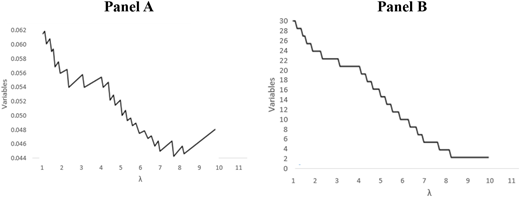
This systematic search ensures that the final model rigorously balances parsimony and explanatory power in a data, -driven manner. Figure 1 illustrates the influence of the regularisation parameter λ on the model structure and parameter estimates. As λ increases, the separation between the $LL$ and $Penλ$ widens, resulting in an elevated value for the first component of the objective function. Concurrently, the number of model factors declines, which reduces the contribution of the second component of the objective function. At the extreme of λ = 0, all variables start from a large baseline value; as λ grows, a pronounced bifurcation is observed. Variables in a subset quickly approach zero, whereas the rest exhibit oscillatory behaviour that eventually dampens. Figure 1, panel A shows that λ typically decreases initially before increasing again, and removing a variable from the model can cause sudden breaks in the GIC. Figure 1, panel B indicates that larger values of λ are associated with a stepwise reduction in the number of variables retained in the model. This behaviour confirms that λ serves as a tuning parameter that balances model complexity against goodness-of-fit, with higher λ values promoting sparser solutions and reduced parameter variance.

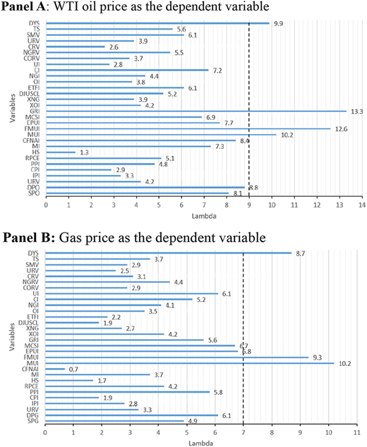
In the study of crude oil price volatility, Figure 2, Panel A, presents the variable inclusion sequence as a function of the penalty parameter λ. Housing starts (HS), crude oil realised volatility (CVR), and unemployment rate (UR) are excluded from the model at λ values of 1.3, 2.6, and 2.8, respectively. This indicates that their contribution to explaining volatility is marginal within the considered framework. Oil-company stock prices and selected uncertainty indices exhibit somewhat stronger effects but are ultimately omitted, suggesting that their influence, while detectable, does not reach a threshold that justifies their retention in the final specification. At λ values of 8.8 and 8.1, the demand-production crude oil (DPO) and supply-production crude oil (SPO) variables are removed from the model, as indicated by the vertical dashed lines in Panel A.

At these points, the objective function attains its minimum when only the last four variables—geopolitical risk uncertainty, financial market uncertainty, macroeconomic uncertainty, and default-yield spread variables—are included. When λ is increased to 9.1, these four variables continue to be selected, underscoring their persistent relevance despite the escalating penalty. Because λ increases monotonically, the analysis does not extend beyond a λ of 13.3. Predictive performance rises predictably in this latter range, and further exploration would not yield additional insights. Consequently, the inference is focused on the λ interval where the critical variables are retained, enabling a parsimonious yet robust description of crude oil price volatility.

Panel B of Figure 2 shows the analysis of natural gas price volatility. This analysis used a regularisation framework to identify the most informative predictors. At the initial λ values of 0.7, 1.7, 1.9, and 1.9, the variables Chicago Fed National Activity (CFNA), Housing Starts (HS), Dow Jones Coal Index (DJUCSL), and Consumer Price Index (CPI) were removed from the regression set. Their exclusion suggests a relatively weak association with natural gas price fluctuations within the examined period. As λ is increased to 6.7 and 6.8, the GRS and MSCI indices are removed from consideration, as evidenced by the vertical dashed lines in Panel B, despite their relatively minor impact on the target variable. Consequently, only the last three predictors remain in the model at these λ values, resulting in the lowest achievable GIC metric performance. At λ = 7, the model retains only the three remaining covariates: Default-Yield Spread (DYS), Financial Market Uncertainty Index (FMUI), and Macroeconomic Uncertainty Index (MUI). The monotonic rise of the GIC beyond this point, as reported in the prior literature, justified ceasing the exploration of higher λ settings.

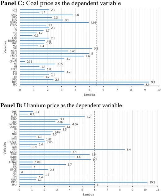
Panels C and D of Figure 2 show the price volatility of coal and uranium, respectively. For coal, the supply (SPC) and demand (DPC) variables exceed a λ threshold of 5.5, ensuring their retention in the predictive model. In contrast, uranium volatility analysis indicates that demand production (DPU) and Geopolitical Risk Index (GRI) surpass a λ of 6.2, thereby being incorporated into the uranium model. Predictors falling below these λ cutoffs for both coal and uranium are systematically excluded; their weaker explanatory contributions are deemed insufficient to materially modify the observed price dynamics. This selective retention underscores the relatively stronger impact of the retained variables on volatility within the respective commodity markets.

After variable selection based on the GIC method, a model is estimated using the selected variables. The long-term volatility component of energy sources can be defined as follows:

1. The long-term crude oil price volatility model can be expressed as follows:

1. The long-term natural gas price volatility model can be expressed as follows:

1. The long-term coal price volatility model can be expressed as follows:

1. The long-term uranium price volatility model can be expressed as follows:

The number of lag periods is 40, which corresponds to data from the previous 40 months (approximately 3 ½ years). All parameter estimates for the energy sources are reported in Tables 1–4. Table 1 shows that the coefficients (ϑ) for the financial market uncertainty, geopolitical risk uncertainty, and macroeconomic uncertainty indices are 0.683, 0.472, and 1.330, respectively. Each coefficient is statistically significant at the 1% level, indicating that increases in any of these uncertainty measures are associated with higher long-term volatility in crude oil prices. The table also presents a ϑ of −1.051 for the default-yield spread, which is significant at the 5% level. This suggests a negative relationship between this credit-risk proxy and long-term oil-price volatility. Together, the results imply that global risk factors—financial, geopolitical, and macroeconomic uncertainties—primarily drive the long-term component of crude oil price volatility through their impact on market expectations about demand, supply, and overall stability. In contrast, the default-yield spread, which reflects cyclical corporate stress and perceived credit risk, exerts a counteracting negative influence. Thus, structural risks associated with global uncertainty appear to have a more pervasive and enduring effect on the risk profile of the crude-oil market than domestic, credit-centric factors.

Table 2 presents the estimated coefficients relating various risk variables to the long-term volatility component of the natural gas price. The coefficients associated with the default-yield spread are 0.548, 0.506 for the financial market uncertainty index, and 1.372 for the macroeconomic uncertainty index. All three coefficients were statistically significant at the 1% level, indicating robust positive relationships. For instance, the coefficient for EPU is 0.223 and is statistically significant only at the 5% level. This suggests a somewhat weaker, albeit still statistically reliable link. Taken together, these results indicate that increases in the default-yield spread, financial market uncertainty index, and macroeconomic uncertainty index are associated with higher long-term volatility in natural gas prices, whereas the effect of economic policy uncertainty is relatively minor.

Table 3 reports estimated ϑ parameters of 0.309 for demand shocks and 0.227 for supply shocks in the coal market, each statistically significant at the 5% level. The estimated demand coefficient indicates that an increase in demand positively contributes to the long-term component of coal price volatility. In contrast, the negative supply coefficient implies that supply shocks exert an opposing long-term influence on volatility.

The econometric results demonstrate that disturbances on both the demand and supply sides substantially increase the volatility of coal prices. The dual-shock sensitivity is consistent with the coal sector's relatively low level of financialisation, which continues to rely heavily on physical market fundamentals rather than being traded in financial markets as often as other energy commodities. Higher industrial demand or alterations in the fuel mix of utilities intensify the responsiveness of coal prices to changes in consumption patterns. On the supply side, disruptions in mining operations, bottlenecks in transportation infrastructure, or policy-driven constraints quickly translate into pronounced price movements due to the limited flexibility of coal production. Taken together, these findings underscore that coal price volatility is fundamentally driven by real sector imbalance. Commodity price dynamics remain tightly coupled with economic and operational variables rather than broader financial or speculative forces.

Table 4 reports the estimated GARCH-type parameters ϑ associated with the uranium demand and the geopolitical risk uncertainty index. The coefficient for the uranium demand index is 0.414 (p < 0.05), whereas that for the geopolitical risk uncertainty index is 0.152 (p < 0.05). Both estimates are positive and statistically significant at the 5% level, indicating that increases in market demand for uranium and in geopolitical risk uncertainty levels increase the long-term component of uranium-price volatility. These results are consistent with the structural characteristics of the uranium market. Production is highly concentrated in a limited number of politically sensitive regions; consequently, any disruption to the geopolitical environment can affect mining, processing, or export routes. When geopolitical risk escalates, market participants adjust their inventory and hedging strategies in anticipation of potential supply curtailments, thereby widening the variance of price changes. Similarly, heightened demand—driven by an expanding nuclear power sector or shifts in utility procurement—exerts upward pressure on prices. Because uranium markets are relatively illiquid and lack the price-absorbing capacity typical of other energy commodities, demand shocks translate into sharper and more persistent volatility. Thus, the empirical analysis demonstrates that uranium-price volatility is jointly determined by supply-side geopolitical risk and demand-side geopolitical risk. The combination of concentrated supply chains and low market liquidity heightens the sensitivity of prices to external factors, resulting in considerable price volatility, as indicated by the estimates.

Eq. (12) is applied for out-of-sample forecasting. To assess the possibility of structural breaks and to gauge the stability and accuracy of the model over time, the entire sample was divided into two periods. The estimation window covers December 2003 to December 2020 and contains 204 monthly observations. In contrast, the forecast-evaluation window runs from January 2021 to March 2024, encompassing 38 months (approximately three years). The proposed model's forecasting performance is benchmarked against three alternative specifications. First, a conventional GARCH model is used. Second, the model is compared with a set of 23 univariate GARCH-MIDAS variants, each of which incorporates only one low-frequency macroeconomic variable. Third, a further GARCH-MIDAS specification incorporates all 28 macroeconomic and policy-related variables simultaneously. The model developed in this study is treated as the benchmark for evaluating forecasting performance and is denoted by $FMRS/FMRSbenchmark$⁠. If the performance ratio is greater than one, it signifies that the benchmark model outperforms the alternative model because of its greater predictive accuracy.

The statistical significance of the performance disparities was assessed using the Giacomini-White (GW) test (Giacomini and White, 2006). Results reported in Tables A3–A6 in the Appendix demonstrate that energy-price models—specifically for crude oil, natural gas, coal, and uranium—exhibit markedly superior out-of-sample performance relative to all benchmark models. Across a range of forecast horizons, the variable-selection GARCH-MIDAS model consistently achieves higher performance ratios, confirming its predictive advantage. Notably, the ratio of forecast errors between the GARCH-MIDAS model and competing models exceeds one, thereby supporting the conclusion of superior predictive performance.

These findings suggest that the integration of low-frequency macroeconomic indicators, measures of economic and financial-policy uncertainty, and high-frequency return data substantially improves volatility-forecasting accuracy. The GW test further confirms that these performance gains are statistically significant at conventional levels (1% and 5%, respectively). Importantly, the results underscore the ability of the GARCH-MIDAS framework to reconcile data observed at different frequencies and to incorporate dynamic structural economic information. Such a feature is particularly valuable for capturing persistent volatility patterns in complex energy markets. Overall, empirical evidence supports the claim that the proposed GARCH-MIDAS model provides a more robust and accurate assessment of commodity-market risk than alternative models documented in the literature (Fang et al., 2020; Liu et al., 2023).

Findings show that the complex economic and financial connections between natural gas market volatility and credit markets explain the positive relationship between natural gas prices and the default-yield spread. Higher natural gas prices usually indicate robust economic activity because natural gas demand tends to rise during periods of economic expansion. While this initially reduces the default risk of energy producers, persistently high prices increase production costs and inflationary pressures, harming energy-intensive sectors and heightening financial stress. This, in turn, raises default-yield spread factor. Higher natural gas prices feed inflation, prompting central banks to raise interest rates to counteract the impact. Higher borrowing costs substantially elevate default risk, especially for economies that rely heavily on energy-intensive industries. This dynamic is exacerbated by heightened investor uncertainty during periods of natural gas price increases. To offset this perceived risk, lenders generally request higher yields. International supply-chain disruptions triggered by natural gas price shocks further intensify these effects, increasing uncertainty and financial market instability. These empirical findings are consistent with earlier studies, including those by Nalban and Smădu (2021).

Conversely, the relationship between crude oil prices and the default-yield spread factor is negatively correlated. Low crude oil prices, caused by high production from major exporters, cut businesses' energy costs, stimulate economic activity, and reduce default risk. In particular, lower crude oil prices benefit energy-intensive industries, lowering their production costs and boosting profitability. Furthermore, lower crude oil prices help dampen inflation, enabling central banks to maintain an accommodative monetary policy. This reduces borrowing costs and eases financial stress.

Although crude oil and natural gas are related commodities, credit markets can react differently to their volatility because of significant structural differences. Crude oil is a highly global and liquid market with deep futures contracts, efficient price discovery, and extensive hedging options. Consequently, oil-price volatility is often absorbed rapidly and does not always lead to substantial credit-risk adjustments. In contrast, natural gas markets tend to be more regional and less liquid, usually settling through long-term or take-or-pay contracts. These characteristics make hedging gas price volatility more difficult and more closely linked to firms' cash-flow risks. Consequently, credit markets view gas shocks as more severe. Other factors, including storage constraints, seasonal demand fluctuations and varying sustainability policies, also accentuate the divergence in credit risk reactions.

These findings confirm the conclusions of earlier studies, including those of Sun et al. (2022). However, in contrast to the results of this study, Szafranek et al. (2020) also found a positive correlation between default-yield spreads and fluctuations in crude oil and natural gas prices. Their analysis reveals a strong positive link between forward-looking market expectations of crude oil price shocks and energy firms' default-yield spread. The study also shows that recent natural-gas price shocks, which have become less closely linked with crude oil prices, are a major factor in explaining default-yield spread fluctuations, highlighting the growing influence of energy markets on default-yield spread patterns.

The analysis indicates a statistically significant positive association between the macroeconomic uncertainty index, financial market uncertainty indices, and crude oil and natural gas prices. In times of heightened macroeconomic and financial uncertainty, investors view crude oil and natural gas as defensive assets against inflation and broader economic instability. This perception enhances the demand for commodities, thereby exerting upward pressure on their prices. Elevated volatility in equity and bond markets stimulates speculative activity in energy commodities, further amplifying price increases. Higher levels of uncertainty further promote speculative trading, which magnifies price fluctuations as investors react more aggressively to new information. Uncertainty also elevates precautionary demand, prompting firms and national governments to build up inventories in anticipation of potential future supply disruptions. The resulting increase in inventory levels contributes to heightened volatility in the spot and futures markets.

Furthermore, uncertainty typically delays energy production and infrastructure investment, reducing supply responsiveness to demand shocks and increasing price sensitivity. Taken together, these mechanisms provide a coherent explanation for the observation that rising uncertainty tends to amplify volatility in the oil and gas markets. These results corroborate the findings of Shi and Shen (2021). The results indicate a positive correlation between the volatility of coal and uranium prices and the respective supply and demand dynamics. This association emphasises the influence of market fundamentals on coal price fluctuations. Research by Gu et al. (2020), for example, has shown that higher demand and limited supply can lead to increased price fluctuations, which are often driven by supply and demand imbalances in energy markets.

The finding that coal volatility is driven almost entirely by its own supply–demand fundamentals indicates that coal is less financially stable than oil and natural gas. Unlike oil and gas, which have substantial futures markets, hedging tools, and speculative positions that closely tie them to global financial systems, coal markets are relatively thin and regionally fragmented. They are primarily governed by bilateral or long-term physical agreements. Consequently, limited financialization causes coal prices to react chiefly to mining output, transportation constraints, and industrial demand, rather than to global macro-financial shocks or investor sentiment.

The positive relationship for uranium extends beyond basic US market forces and extends into geopolitical uncertainty. Lyócsa and Todorova (2024) showed that geopolitical tensions, policy changes, and international trade restrictions have a significant impact on uranium markets in their analysis of uranium price sensitivity to political instability and international energy security concerns.

For uranium, the strong effect of geopolitical risk is expected because its supply chain is highly concentrated, tightly regulated, and sensitive to strategic tensions. Kazatomprom, for example, is the world's largest uranium producer and plays a pivotal role in global supply, meaning that political or operational disruptions in Kazakhstan are immediately reflected in prices. Similarly, instability in Niger, another major producer, has historically triggered supply concerns and price spikes. Energy security issues involving US dependence on Russian-enriched uranium, especially under sanctions or export restrictions, also heighten volatility. It is underlined that uranium markets are shaped more by geopolitical constraints, regulatory decisions, nuclear-policy shifts, and security alliances than by conventional financial flows.

The present study builds directly on the work of Pastor and Veronesi (2012), who highlighted the significant impact of government policy uncertainty on financial markets. This study introduces a new approach for identifying key drivers of financial price volatility by employing a GARCH-MIDAS framework with an adaptive LASSO penalty for variable selection, which expands the methodological toolbox for energy economics research. The findings challenge conventional supply-and-demand explanations of market fluctuations (Hamilton, 1983; Kilian, 2009), indicating that uncertainty measures have a greater impact in today's financialized economy marked by volatile energy markets. Furthermore, this paper enriches the theoretical understanding of commodity market financialisation by demonstrating that macroeconomic and financial market conditions increasingly shape prices of major energy sources rather than solely by physical demand supply dynamics (Anand and Paul, 2021). This aligns with the view that integrating energy markets into global financial systems heightens the role of uncertainty as a pivotal driving factor (Tong et al., 2023).

Academic analyses of the factors that determine energy prices have changed noticeably over time. From the early decades of the 20th century until the late 20th century, the control and distribution of energy were largely centralised within groups such as OPEC, as well as within major producing and exporting nations. Together, these actors had a decisive influence on energy markets, and scholars of the period largely agreed that prices were “supply-driven” (Dees et al., 2007). By the middle of the century, rapid growth in several emerging economies and a growing demand for energy led scholars to shift their focus to a “demand-driven” framework, as highlighted by Kilian (2009). In recent years, price movements have become increasingly linked to financial markets, producing large fluctuations that reflect market expectations and speculative behaviour. Macroeconomic uncertainty has emerged as a key driver of these dynamics, with critical events such as the Global Financial Crisis, the COVID-19 pandemic, and the latest geopolitical tensions between Russia and OPEC as well as between Russia and Ukraine exerting significant influence.

These conflicts have increased volatility by disrupting supply chains and raising doubts about future availability and pricing. While the complex mechanisms behind energy price volatility remain to be fully understood, this study finds that uncertainty, particularly that stemming from financial market, geopolitical and economic instability, has the strongest effect on price movements. Accordingly, the study offers several recommendations: when forecasting the prices of crude oil, natural gas, coal, and uranium, market participants should give priority to evaluating financial-market, geopolitical, and macroeconomic uncertainties in order to enhance the effectiveness of risk-management approaches. Through thorough analysis, uncertainties influencing energy-price dynamics can be mitigated, thereby minimising potential risks. Investors, policymakers, and analysts can gain valuable insights into future price trends, monetary policy, and market conduct by doing so.

This study has limitations that provide avenues for future research. First, the analysis focuses solely on macro-level factors, overlooking key micro-level variables such as technological progress in energy production and firm-specific energy consumption patterns. Investigating these variables would yield a broader understanding of what drives major energy sources' price volatility. Second, the study takes a global view of energy markets while ignoring the regional specificity of emerging markets, where factors, including currency volatility, local energy policies, and government subsidies, can markedly influence price volatility. A region-specific approach would offer deeper insight into these distinct determinants. Finally, the study fails to examine the increasing influence of carbon pricing, low-emission energy policies, and international decarbonisation initiatives on energy prices. With the rapid energy transition and worldwide emphasis on sustainability, future research should explore how these elements shape energy price dynamics.

Several macroeconomic variables are hypothesised to affect energy price volatility. This study investigates which of these variables exerts the strongest influence on the corresponding economic indicators. A GARCH-MIDAS regression framework is employed, augmented with a log-likelihood function that incorporates an adaptive LASSO penalty. By maximising this penalised log-likelihood subject to linear constraints, the model isolates the primary determinants for each energy source. For crude-oil volatility, the default-yield spread, the geopolitical risk uncertainty index, the macroeconomic uncertainty index, and the financial market uncertainty index are identified as the most influential drivers. A similar pattern emerges for natural-gas price volatility, where the default-yield spread, the financial market uncertainty index, and the macroeconomic uncertainty index also show statistical significance. In the case of coal, the interaction between supply and demand is found to be the principal determinant of price volatility. Finally, two factors—uranium demand and the geopolitical risk uncertainty index—predominate as the main influencers of uranium-energy price volatility.

The supplementary material for this article can be found online.