

The study investigates the impact of inflation-targeting monetary policies on financial stability across developed and emerging economies, addressing a critical gap in understanding their broader implications beyond price stability. It aims to assess the ability of inflation-targeting regimes to sustain financial stability in diverse economic contexts.
The research employs survival analysis techniques, including Kaplan–Meier estimation and the Cox proportional hazards model, to analyse panel data from 13 countries (six developed and seven emerging economies) over 23 years. A Macro-Financial Stability Index is constructed using macroeconomic, stock market and banking-sector variables, with non-parametric and semi-parametric methods estimating survival functions and hazard ratios.
The findings reveal differences between developed and emerging economies. Developed economies demonstrate higher survival probabilities, reflecting resilience to financial instability due to robust institutional frameworks. Emerging economies show more rapid declines in survival probabilities, highlighting vulnerabilities to external shocks and economic volatility.
The study is limited to 13 countries over 23 years, excluding other inflation-targeting experiences. Expanding the dataset could enhance the findings. Results underscore the need for tailored inflation-targeting policies to address the distinct challenges of emerging economies.
This study applies survival analysis to assess the duration of financial stability under inflation-targeting regimes, offering a comparative analysis of developed and emerging economies. It highlights the importance of integrating macroprudential measures into monetary policy, for enhancing resilience in emerging markets.
1. Introduction
Financial stability has become a central concern in monetary policy because price stability on its own does not guarantee broader economic stability. Financial stability is commonly understood as a financial system that functions efficiently and can absorb shocks while maintaining confidence and supporting sustainable growth (Borio and Drehmann, 2009). This perspective has widened the role of central banks beyond inflation control toward safeguarding both macroeconomic performance and the soundness of the financial system (Mishkin and Eakins, 2016).
Within the main monetary policy strategies outlined by Mishkin, inflation targeting is a leading framework alongside exchange rate targeting, monetary targeting and approaches that are not anchored to a single indicator (Mishkin, 2009). Inflation targeting began with the Reserve Bank of New Zealand in 1990 and has since spread across developed economies such as Australia, Norway and Israel, and emerging economies such as South Africa, Brazil and Chile (Guo, 2024). In practice, central banks publicly announce an inflation target, often around 2%, and adjust short-term interest rates and other instruments when inflation moves away from the target. A stable inflation environment can improve predictability in financial markets, support investment and strengthen confidence in the monetary regime (Schwartz, 1998; Adrian et al., 2018).
However, experiences from the 2008 global crisis and the COVID-19 shock reinforced that monetary policy and financial risks are tightly connected, prompting stronger macroprudential action and, in some cases, unconventional policies such as quantitative easing and negative interest rates to ease liquidity strains and stabilise recovery (Aikman et al., 2019; Borio et al., 2023; Gertler and Karadi, 2011; Brunnermeier et al., 2020). A resilient financial system matters for efficient resource allocation and for the transmission of policy, especially during periods of severe disruption (Mishkin, 2011; Acharya and Steffen, 2020). At the same time, inflation targeting may, under certain conditions, coincide with rising vulnerabilities, for example when low rates support risk taking, credit booms or asset price inflation even while inflation remains contained (Woodford, 2012; Giavazzi and Giovannini, 2010; Tobal and Menna, 2020). Related work recognises inflation targeting’s credibility gains but notes its limits in preventing financial imbalances such as credit surges and bubbles (Cecchetti, 2016; Blanchard et al., 2013).
A key gap is that much of the literature emphasises inflation outcomes while paying less attention to how long financial stability can be sustained under inflation targeting across different contexts. Mishkin (2009) and Roger (2010) stress inflation control, while evidence from major shocks raises questions about financial resilience under these regimes. Cross-country studies such as Vega and Winkelried (2005) and Gonçalves and Salles (2008) compare developed and emerging economies yet provide limited insight into the time profile of financial stability after adoption. This motivates the present study, which compares emerging and developed inflation targeting economies and uses survival analysis to examine the duration of financial stability and how it is shaped by financial development, institutional strength and external vulnerabilities. Survival analysis is well suited to time to event questions and allows covariates to explain why stability persists or fails, with group differences assessed using log rank and Wilcoxon tests.
The remainder of this study is structured as follows: Section 2 presents the literature review; Section 3 outlines the research methodology and describes the data and variables used. Section 4 provides the empirical results and discussion, and Section 5 concludes with key findings and policy recommendations.
2. Literature review
Recent work builds on New Keynesian Dynamic Stochastic General Equilibrium (DSGE) models to explain why inflation targeting cannot be studied in isolation from financial stability, particularly after the 2008 Global Financial Crisis exposed gaps in standard monetary frameworks. Earlier DSGE setups focused on stabilising inflation around a target, while smoothing output fluctuations through Taylor rule type responses. Newer models add financial frictions, such as credit constraints and banking sector dynamics, to show how credit and asset price shocks can amplify macroeconomic volatility and make it more difficult for policy to deliver both price and financial stability at the same time (Bauducco et al., 2014). One line of argument is to extend the Taylor rule by including financial stability indicators such as credit growth or leverage, so monetary policy leans against the wind when risks build up (Woodford, 2012). In this setting, macroprudential instruments, including countercyclical capital buffers and loan-to-value (LTV) limits, can be layered onto inflation targeting to reduce systemic risk without abandoning the inflation target itself. Overall, the DSGE literature points toward a broader policy mix where monetary policy and macroprudential regulation work together to manage instability risks that, if ignored, can later threaten price stability (Brunnermeier and Sannikov, 2014).
Evidence from developed economies uses a range of empirical approaches and often reaches mixed conclusions about whether inflation targeting supports financial stability. For Norway, Akram and Eitrheim (2008) use time series analysis and find that inflation targeting can help stabilise financial markets while remaining consistent with price stability, echoing the broader case for predictable inflation in Schwartz (1998). In the Euro Area, Cassola and Morana (2004) employ a sign restrictive vector autoregression to study the interaction between monetary and financial stability after shocks, although results depend on identifying assumptions. Frappa and Mésonnier (2010) apply propensity score methods to 17 Organisation for Economic Co-operation and Development (OECD) countries and suggest that inflation targeting may coincide with greater financial fragility, partly through housing price booms, even if matching helps reduce selection bias. In the United States context, Taylor (2009) uses counterfactual analysis to argue that policy rates held below Taylor rule prescriptions contributed to the housing boom of the 2000s, while Detken and Smets (2004) show across asset price boom episodes that accommodative policy can raise longer run costs when prices eventually adjust. Related studies by Rigobon and Sack (2003) and Bohl and Siklos (2008) indicate that central banks respond more strongly when asset prices deviate sharply from perceived equilibrium, suggesting a non-linear policy reaction, even if such models cannot fully capture the real world complexity of policy making.
In emerging economies, the literature places greater weight on macroprudential policy as a practical complement to inflation targeting, especially where financial markets are more volatile. Using bank level and country level panel data, Fendoglu (2017) and Kuttner and Shim (2016) find that tools such as LTV and debt to income limits can kerb housing credit growth and dampen house price inflation in emerging markets relative to developed economies. Bulíř and Čihák (2008), using panel regressions for emerging and selected advanced economies, show that central banks often respond asymmetrically to financial stress, easing more aggressively in crises than tightening in booms, a pattern that may intensify instability. Angelini et al. (2014) argue, using theory and empirical evidence, that coordinating macroprudential tools, including higher capital requirements, with monetary policy can reduce sensitivity to interest rate movements and improve outcomes, though the breadth of inference is limited by the small number of cases examined. More generally, macroprudential instruments such as capital requirements, LTV ratios and countercyclical buffers are seen as central to restraining credit booms and stabilising asset prices (Fendoglu, 2017; Kuttner and Shim, 2016). Yet Cecchetti and Li (2008) caution that tensions can arise when tighter macroprudential constraints weaken credit supply and dampen the effects of accommodative interest rate policy. More recent thinking stresses that strong macroprudential frameworks can actually expand monetary policy room for manoeuvre by limiting the risks created by prolonged low interest rates, thereby strengthening financial stability within inflation targeting regimes (Borio et al., 2023).
Against this background, the review highlights a gap in how the inflation targeting and financial stability literature connect over time. Studies such as Vega and Winkelried (2005) and Gonçalves and Salles (2008) emphasise inflation targeting’s role in lowering inflation volatility but give less attention to long-run financial stability implications. Methodologically, much of the evidence relies on time series analysis and vector autoregressions, which are less suited to modelling duration, handling censored observations or tracking how stability evolves under shifting macroeconomic conditions. The study responds by applying survival analysis to the time to financial instability under inflation targeting, positioning this as a novel contribution in this area and using the framework to draw out policy lessons for both emerging and developed economies.
The study’s contribution is framed in three parts. First, it constructs a macro financial stability index that combines macroeconomic indicators with stock market and banking sector variables, offering a broader stability measure than studies focused on a single segment. Second, it applies survival analysis tools, including Kaplan–Meier estimators and Cox proportional hazards models, to assess the duration of financial stability under inflation targeting across developed and emerging economies, explicitly modelling time to instability and accounting for censored data. Third, it compares how structural factors, including liquidity conditions, net foreign assets and interest rates, shape instability risk across country groups, tying the inflation targeting debate more directly to macroprudential policy and institutional quality.
3. Methodology and data
3.1 Survival analysis
This study uses survival analysis to examine how long inflation targeting economies are able to maintain financial stability before a disruption occurs. Survival analysis focuses on time to event outcomes, meaning it models the duration until a defined event such as the onset of financial instability or a policy regime shift (Guo and Lim, 2024; Collett, 2023). Because many countries may not experience the event within the sample window, the approach is designed to handle censored observations, which helps avoid losing information when the event has not occurred by the end of the study period (Klein and Moeschberger, 2006; Zhuhadar et al., 2019). This makes it a good fit for cross-country comparisons, where the timing of instability and the pace of regime change can differ across developed and emerging economies. It also allows the study to quantify how policy and structural conditions shape risk over time, including the role of macroprudential measures that may extend stability in more shock exposed settings (Fendoglu, 2017). The framework is presented as more informative than standard time series methods for capturing duration and timing, especially when events are infrequent or conditions shift sharply (Collett, 2023; Kleinbaum and Klein, 2012).
3.2 Basic concepts and methods
For estimation, the study combines non-parametric and semi-parametric tools. The Kaplan–Meier estimator is used to trace survival functions and compare how the probability of remaining financially stable evolves over time, while accommodating right censoring. Since Kaplan–Meier does not include covariates, the Cox Proportional Hazards Model is then applied to evaluate how explanatory variables affect the hazard rate, without imposing a specific distribution on survival times. This structure makes it possible to test how factors such as macroprudential policies and interest rates relate to the risk of moving into instability. The methodology is supported with standard diagnostics. The Schoenfeld residuals test is used to assess the proportional hazards assumption in the Cox model and deviance residuals help identify influential observations. For Kaplan–Meier results, independent censoring assumptions and log-rank tests are used to validate estimates and compare survival curves across groups.
3.2.1 Survival analysis and nonparametric model estimation
3.2.1.1 Survival functions
For any time, t, let T be a continuous random variable representing the time until the occurrence of an event of interest, with f(t) as its probability density function. The survival function is defined as
The function in equation (3.1) represents the probability that the event of instability does not occur by time t, meaning that financial stability is “surviving” up to that point. The f(t) provides the likelihood of the event of instability occurring exactly at time t. F(t) is the cumulative probability that the event has already occurred by time t, capturing the probability of a country experiencing financial instability up to time t. Then, 1−F(t) calculates the probability that a country has not yet encountered instability by time t.
The hazard function, equation (3.2), also referred to as the risk function or intensity rate which is denoted by ℎ(t), is defined as the rate at which a country experiences the event within a small-time interval Δt, given that the event has not occurred up to time t (Chen, 1996). Specifically, it represents:
3.2.1.2 Kaplan–Meier estimate of survival function
The Kaplan–Meier estimator, introduced by Kaplan and Meier (1958), is a nonparametric method for estimating the survivor function (t), which represents the probability of surviving beyond time t, or equivalently, the probability of experiencing the event after time t. Among the n countries, some might experience right censoring, and multiple countries could share the same survival time.
The survival analysis approach is applied to estimate the time until financial instability occurs within developed and emerging economies under inflation targeting regimes. The survival times represent distinct even times in ascending order, where < ….< . The variable defines the number of economies that transition into instability right before . The probability of instability for an economy by time is calculated as , and the probability of remaining stable (or “surviving”) by that same time is 1 − . This approach aligns with Collet’s (2023) formulation, which presents the survival function as any time t in the interval from to supporting the Kaplan–Meier estimation method.
For t with = 1 an
d = 0. The result in equation (3.3) is known as the Kaplan–Meier estimate of survival function at t.
The standard error of the Kaplan–Meier estimate of the survival function is given by
The 100(1 − α)% confidence interval for the survival function, S(t), is
where is given by formula 3.4, is the upper - point of the standard normal distribution.
3.2.1.3 The log-rank test for two groups
The log-rank test evaluates whether Kaplan–Meier survival curves differ across groups. In this study, the comparison is restricted to two groups. Statistical equivalence indicates that the test provides insufficient evidence that the underlying population survival distributions differ.
Comparing group I (Developed countries) to group II (Emerging economies), Collet (2023) reports the log-rank test as follows:
Consider r interval of time for each group for j = 1, 2, … r.
Denote:
, the number of events (financial instability) from group II at time
, the number of countries in group I at risk before time ,
, the number of countries in group II at risk before time .
The total number of countries at risk at time is = + while the total number
of events at time is = + .
The null and alternative hypotheses are now formulated as follows:
no difference in survival experiences between the two groups.
there is difference in survival experiences between the two groups.
The log-rank test is appropriate for proportional hazards function, that is when the plots of the estimates of the survival function for the two groups are approximately parallel (Collet, 2023).
3.3 Data and data sources
The data come primarily from the World Bank World Development Indicators database (World Bank, 2024), supplemented by publicly available central bank sources. The sample covers 13 inflation targeting countries from 2001 to 2023, split into six developed and seven emerging economies. Countries are chosen based on three main conditions. They must have maintained a clear and sufficiently long inflation targeting regime to make duration analysis meaningful. They must have consistent macroeconomic, stock market and banking sector data available across the full period so that the macro financial stability index is comparable. They must also collectively reflect institutional and geographic diversity, allowing differences in survival times to be interpreted through structural heterogeneity rather than isolated country stories. The final dataset contains 138 observations for developed economies and 161 for emerging economies, providing a basis for longitudinal comparison. Variable definitions are reported in Table 1.
Variable description
| Variables | Description | Codes | Sources |
|---|---|---|---|
| Trade (% of GDP) | Represents the sum of exports and imports as a percentage of a country’s GDP, indicating the degree of openness and external integration of the economy | TGDPG | World Bank (WDI) |
| GDP (constant LCU) – LN | The total market value of all goods and services produced within a country, measured in constant local currency units (LCU), adjusted for inflation to show real growth | DGPCG | World Bank (WDI) |
| GDP growth (annual %) | The annual percentage increase in a country’s GDP, reflecting the pace of economic expansion or contraction over time | GDPG | World Bank (WDI) |
| GDP per capita (constant LCU) – LN | The average economic output per person, measured in constant local currency units, providing insight into the standard of living and economic prosperity | GDPPG | World Bank (WDI) |
| Inflation, consumer prices (annual %) | The annual percentage change in the cost of a basket of goods and services typically consumed by households, indicating price stability or instability | INFG | World Bank (WDI) |
| Inflation, GDP deflator (annual %) | Measures the change in prices for all goods and services in an economy, comparing the nominal GDP to real GDP and providing a broader inflation measure than consumer prices | INFDG | World Bank (WDI) |
| Real effective exchange rate index (2010 = 100) | An index measuring the value of a country’s currency relative to a weighted average of its trading partners’ currencies, adjusted for inflation differentials, indicating international competitiveness | REEG | World Bank (WDI) |
| Law and order | An index assessing the strength of the legal framework and the level of adherence to the rule of law within a country, crucial for institutional stability and investor confidence | LOG | World Bank (WDI) |
| Market capitalisation of listed domestic companies (% of GDP) | The total value of a company’s shares of stock, reflecting the overall size of the stock market relative to the economy and investor sentiment toward public equities | MCG | World Bank (WDI) |
| Stocks traded, total value (% of GDP) | The total number of shares traded during a given period, showing the liquidity and trading activity within the stock market | STG | World Bank (WDI) |
| Net foreign assets (current LCU) – LN | The value of foreign assets held by domestic banks minus foreign liabilities, providing insights into the banking sector’s exposure to global financial markets and external shocks | NFAG | World Bank (WDI) |
| Lending interest rate (%) | The interest rate charged by banks on loans to the private sector, indicating the cost of borrowing and the credit conditions in the economy | LIG | World Bank (WDI) |
| Deposit interest rate (%) | The interest rate paid by banks on deposits, reflecting the incentives for saving and the cost of holding funds in the banking system | DIG | World Bank (WDI) |
| Broad money (% of GDP) | The total amount of money in circulation, including cash, checking deposits and easily accessible financial instruments, used as an indicator of overall liquidity in the economy | M3G | World Bank (WDI) |
| Bank liquid reserves to bank assets ratio (%) | The proportion of banks’ liquid assets (cash and readily convertible securities) relative to total assets, indicating the banking sector’s ability to meet short-term obligations and maintain financial stability | BLRG | World Bank (WDI) |
Note(s): WDI represents world development indicators
4. Results and discussions
The study begins by presenting the model fit and diagnostic tests, which were analysed using the log-rank and Schoenfeld residual tests. These results are crucial as they validate the proportional hazards assumption, a key aspect of the Cox regression model. The log-rank test evaluates whether survival curves differ between groups, while the Schoenfeld residual test detects any non-proportionality in covariates, ensuring that the impact of variables on the hazard rate remains consistent over time.
4.1 The log-rank test and Schoenfeld residual test
4.1.1 Log-rank test
The log-rank test results in Table 2 reveal differences in survival times between developed and emerging economies, with a chi-squared value of 266.45, highly significant at 1%. This suggests substantial differences in the survival experiences of these groups. The test highlights consistent deviations from expected event counts, confirming a statistically significant divergence in survival patterns that warrants further investigation.
Log-rank test and the Wilcoxon test
| Variable | Log-rank test statistic (p-value) | Wilcoxon test statistic (p-value) |
|---|---|---|
| INFG | 266.45 (0.0000) | 223.31 (0.0000) |
| STG | 266.45 (0.0000) | 223.31 (0.0000) |
| M3G | 266.45 (0.0000) | 223.31 (0.0000) |
Similarly, the Wilcoxon–Breslow–Gehan test compares survival functions between the two groups, yielding a chi-squared value of 223.31, which rejects the null hypothesis of equal survival distributions. The results for stock trading growth (STG) and M3G mirror those of INFG, with chi-squared values and p-values confirming significant differences between developed and emerging economies across all three variables. This consistency across tests reinforces the robustness of the findings and the clear divergence in survival patterns.
4.1.2 Schoenfeld residual Test
The results in Table 3 present the Schoenfeld test in the banking sector of emerging economies; it confirms that the proportional hazards assumption holds for all variables. The p-values for M3G (0.8869), net foreign assets growth (NFAG) (0.8281), LIG (0.5209), bank liquid reserves growth (BLRG) (0.2655) and DIG (0.2479) all exceed the 0.05 threshold, indicating their effects on financial stability duration remain constant over time. The global test p-value of 0.6313 further supports this, confirming that no violations exist for the model. As such, no adjustments, such as stratification or time-varying covariates, are required.
Schoenfeld residual test results for the banking sector
| Variable | Prob > χ2 |
|---|---|
| M3G | 0.8869 |
| NFAG | 0.8281 |
| LIG | 0.5209 |
| BLRG | 0.2655 |
| DIG | 0.2479 |
| Global test | 0.6313 |
The results in Table 4 show, for stock market variables, that market capitalisation growth (MCG) (0.9337) and STG (0.2502) provide no evidence of non-proportionality, indicating time-independent effects on financial stability.
Schoenfeld residual test results for the stock markets
| Variable | Prob > χ2 |
|---|---|
| MCG | 0.9337 |
| STG | 0.2502 |
| Global test | 0.5162 |
In terms of macroeconomic variables presented in Table 5, the proportional hazards assumption holds for TGDPG (0.7771), GDPCG (0.3991), GDP growth (GDPG) (0.8498), GDPPG (0.4828), INFG (0.8247), INFDG (0.7935) and LOG (0.4528). However, REEG (0.0616) shows slight evidence of non-proportionality, suggesting that its effect may change slightly over time. The global test p-value of 0.4746 indicates that the model fits well overall, but REEG might benefit from further exploration for potential time-varying effects.
Schoenfeld residual test results for the macroeconomic level
| Variable | Prob > χ2 |
|---|---|
| TGDPG | 0.7771 |
| GDPCG | 0.3991 |
| GDPG | 0.8498 |
| GDPPG | 0.4828 |
| INFG | 0.8247 |
| INFDG | 0.7935 |
| REEG | 0.0616 |
| LOG | 0.4528 |
| Global test | 0.4746 |
The study also presents the results of the Schoenfeld Residual Test, in developed countries. Table 6 illustrates the test results in the banking sector of developed economies, where M3G (0.9135), LIG (0.6615) and DIG (0.5779) demonstrate no non-proportionality, with constant effects on financial stability over time. The global test p-value of 0.0641 shows borderline evidence of non-proportionality, suggesting that the model mostly holds but may require further examination.
Schoenfeld residual test for the banking sector
| Variable | Prob > χ2 |
|---|---|
| M3G | 0.9135 |
| NFAG | 0.0078 |
| LIG | 0.6615 |
| BLRG | 0.0092 |
| DIG | 0.5779 |
| Global test | 0.0641 |
Additionally to the variables in developed countries, Table 7 shows results for the stock market variables, where MCG (0.7846) and STG (0.9794) show no evidence of non-proportionality. The global test p-value of 0.9583 confirms that the model captures their time-independent effects.
Schoenfeld residual test for the stock market
| Variable | Prob > χ2 |
|---|---|
| MCG | 0.7846 |
| STG | 0.9794 |
| Global test | 0.9583 |
Lastly, among macroeconomic variables, in Table 8, the variables TGDPG (0.5077), GDPCG (0.4798), GDPG (0.3970), GDPPG (0.8385), INFG (0.9839), REEG (0.1405) and LOG (0.1737) show no signs of non-proportionality. INFDG (0.0644) presents borderline evidence of non-proportionality, suggesting a potential, though not significant, time-varying effect.
4.2 Kaplan–Meier
4.2.1 Kaplan–Meier: banking sector
In developed economies, M3G shows gradual declines, reflecting stable liquidity management and balanced money supply, while emerging economies experience sharper declines, indicating vulnerability to liquidity shocks shown in Figure 1. Strengthened monetary policies are needed in emerging economies to manage liquidity effectively. For NFAG, developed economies demonstrate stable foreign asset management, while emerging economies face greater exposure to currency risks and external debt.
 Ten panels are shown in five rows and two columns. Panel a) M 3 G – Dev Econ: The graph titled “Kaplan–Meier survival estimate” shows survival probability over time in years. The horizontal axis is labeled “Time (years)” and ranges approximately from 2000 to 2025 in increments of 5 years. The vertical axis is labeled “Survival probability” and ranges from 0 to 1 in increments of 0.25. Two lines are displayed: a dashed line labeled “95 percent C I” and a solid blue line labeled “Survival function”. The survival curve begins near 1.0 around the year 2000 and declines steadily in a stepwise pattern across the period, approaching 0 by 2023. The dashed confidence interval bands follow closely above and below the survival function throughout. Panel b) M 3 G – Emerg Econ: The graph titled “Kaplan–Meier survival estimate” shows survival probability over time in years. The horizontal axis is labeled “Time (years)” and ranges approximately from 2000 to 2025 in increments of 5 years. The vertical axis is labeled “Survival probability” and ranges from 0 to 1 in increments of 0.25. Two lines are shown: a dashed line labeled “95 percent C I” and a solid blue line labeled “Survival function”. The survival curve starts near 1.0 around 2000 and declines gradually in stepwise form, reaching a low value near 0 by 2020. The dashed confidence intervals closely track the survival curve throughout the period. Panel c) N F A G – Dev Econ: The graph titled “Kaplan–Meier survival estimate” displays survival probability over time in years. The horizontal axis ranges approximately from 2000 to 2025 in increments of 5 years. The vertical axis ranges from 0 to 1 in increments of 0.25. The solid blue line labeled “Survival function” begins near 1.0 and decreases steadily across time. The dashed “95 percent C I” lines remain narrowly distributed around the survival function. The survival probability approaches 0 by the end of the observed period. Panel d) N F A G – Emerg Econ: The graph titled “Kaplan–Meier survival estimate” shows survival probability across time. The horizontal axis ranges approximately from 2000 to 2025 in increments of 5 years. The vertical axis ranges from 0 to 1 in increments of 0.25. The survival function begins near 1.0 and declines in a stepped downward pattern over time. The dashed confidence interval lines follow the survival curve and widen slightly in later years. The survival probability decreases toward 0 by the final years. Panel e) L I G – Dev Econ: The graph titled “Kaplan–Meier survival estimate” presents survival probability over time. The horizontal axis ranges from approximately 2000 to 2025 in increments of 5 years. The vertical axis ranges from 0 to 1 in increments of 0.25. The solid survival function line begins near 1.0 and declines steadily in a staircase pattern. The dashed “95 percent C I” lines remain close to the survival function throughout. The survival probability approaches near 0 by 2020. Panel f) L I G – Emerg Econ: The graph titled “Kaplan–Meier survival estimate” shows survival probability across time. The horizontal axis ranges approximately from 2000 to 2025 in increments of 5 years. The vertical axis ranges from 0 to 1 in increments of 0.25. The solid blue survival function starts near 1.0 and declines steadily across the years. The dashed 95 percent confidence interval lines follow the survival function closely. The curve trends downward toward 0 by the final period. Panel g) D I G – Dev Econ: The graph titled “Kaplan–Meier survival estimate” displays survival probability over time. The horizontal axis ranges approximately from 2000 to 2025 in increments of 5 years. The vertical axis ranges from 0 to 1 in increments of 0.25. The solid survival curve starts near 1.0 and declines stepwise across the period. The dashed confidence interval lines remain near the survival curve. Survival probability decreases toward 0 by the end of the time span. Panel h) D I G – Emerg Econ: The graph titled “Kaplan–Meier survival estimate” shows survival probability across time. The horizontal axis ranges approximately from 2000 to 2025 in increments of 5 years. The vertical axis ranges from 0 to 1 in increments of 0.25. The solid blue survival function begins near 1.0 and decreases steadily in steps. The dashed 95 percent confidence intervals follow closely. The survival probability approaches low values near 0 in later years. Panel i) B L R – Dev Econ: The graph titled “Kaplan–Meier survival estimate” presents survival probability over time. The horizontal axis ranges from approximately 2000 to 2025 in increments of 5 years. The vertical axis ranges from 0 to 1 in increments of 0.25. The survival function starts near 1.0 and declines progressively over the years. The dashed 95 percent confidence interval lines track the survival curve closely. The curve approaches 0 by the final observed year. Panel j) B L R – Emerg Econ: The graph titled “Kaplan–Meier survival estimate” shows survival probability over time. The horizontal axis ranges approximately from 2000 to 2025 in increments of 5 years. The vertical axis ranges from 0 to 1 in increments of 0.25. The solid blue survival function begins near 1.0 and declines in a stepwise downward pattern across the period. The dashed 95 percent confidence intervals follow the survival function closely. The survival probability decreases toward 0 in the final years.
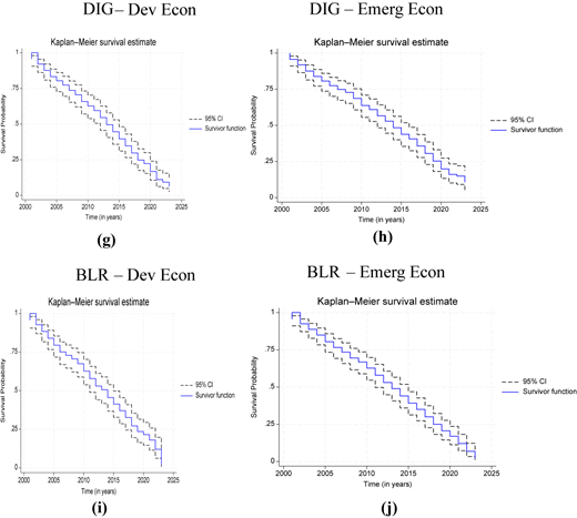
Kaplan–Meier: banking sector. Source(s): Authors’ own work
Ten panels are shown in five rows and two columns. Panel a) M 3 G – Dev Econ: The graph titled “Kaplan–Meier survival estimate” shows survival probability over time in years. The horizontal axis is labeled “Time (years)” and ranges approximately from 2000 to 2025 in increments of 5 years. The vertical axis is labeled “Survival probability” and ranges from 0 to 1 in increments of 0.25. Two lines are displayed: a dashed line labeled “95 percent C I” and a solid blue line labeled “Survival function”. The survival curve begins near 1.0 around the year 2000 and declines steadily in a stepwise pattern across the period, approaching 0 by 2023. The dashed confidence interval bands follow closely above and below the survival function throughout. Panel b) M 3 G – Emerg Econ: The graph titled “Kaplan–Meier survival estimate” shows survival probability over time in years. The horizontal axis is labeled “Time (years)” and ranges approximately from 2000 to 2025 in increments of 5 years. The vertical axis is labeled “Survival probability” and ranges from 0 to 1 in increments of 0.25. Two lines are shown: a dashed line labeled “95 percent C I” and a solid blue line labeled “Survival function”. The survival curve starts near 1.0 around 2000 and declines gradually in stepwise form, reaching a low value near 0 by 2020. The dashed confidence intervals closely track the survival curve throughout the period. Panel c) N F A G – Dev Econ: The graph titled “Kaplan–Meier survival estimate” displays survival probability over time in years. The horizontal axis ranges approximately from 2000 to 2025 in increments of 5 years. The vertical axis ranges from 0 to 1 in increments of 0.25. The solid blue line labeled “Survival function” begins near 1.0 and decreases steadily across time. The dashed “95 percent C I” lines remain narrowly distributed around the survival function. The survival probability approaches 0 by the end of the observed period. Panel d) N F A G – Emerg Econ: The graph titled “Kaplan–Meier survival estimate” shows survival probability across time. The horizontal axis ranges approximately from 2000 to 2025 in increments of 5 years. The vertical axis ranges from 0 to 1 in increments of 0.25. The survival function begins near 1.0 and declines in a stepped downward pattern over time. The dashed confidence interval lines follow the survival curve and widen slightly in later years. The survival probability decreases toward 0 by the final years. Panel e) L I G – Dev Econ: The graph titled “Kaplan–Meier survival estimate” presents survival probability over time. The horizontal axis ranges from approximately 2000 to 2025 in increments of 5 years. The vertical axis ranges from 0 to 1 in increments of 0.25. The solid survival function line begins near 1.0 and declines steadily in a staircase pattern. The dashed “95 percent C I” lines remain close to the survival function throughout. The survival probability approaches near 0 by 2020. Panel f) L I G – Emerg Econ: The graph titled “Kaplan–Meier survival estimate” shows survival probability across time. The horizontal axis ranges approximately from 2000 to 2025 in increments of 5 years. The vertical axis ranges from 0 to 1 in increments of 0.25. The solid blue survival function starts near 1.0 and declines steadily across the years. The dashed 95 percent confidence interval lines follow the survival function closely. The curve trends downward toward 0 by the final period. Panel g) D I G – Dev Econ: The graph titled “Kaplan–Meier survival estimate” displays survival probability over time. The horizontal axis ranges approximately from 2000 to 2025 in increments of 5 years. The vertical axis ranges from 0 to 1 in increments of 0.25. The solid survival curve starts near 1.0 and declines stepwise across the period. The dashed confidence interval lines remain near the survival curve. Survival probability decreases toward 0 by the end of the time span. Panel h) D I G – Emerg Econ: The graph titled “Kaplan–Meier survival estimate” shows survival probability across time. The horizontal axis ranges approximately from 2000 to 2025 in increments of 5 years. The vertical axis ranges from 0 to 1 in increments of 0.25. The solid blue survival function begins near 1.0 and decreases steadily in steps. The dashed 95 percent confidence intervals follow closely. The survival probability approaches low values near 0 in later years. Panel i) B L R – Dev Econ: The graph titled “Kaplan–Meier survival estimate” presents survival probability over time. The horizontal axis ranges from approximately 2000 to 2025 in increments of 5 years. The vertical axis ranges from 0 to 1 in increments of 0.25. The survival function starts near 1.0 and declines progressively over the years. The dashed 95 percent confidence interval lines track the survival curve closely. The curve approaches 0 by the final observed year. Panel j) B L R – Emerg Econ: The graph titled “Kaplan–Meier survival estimate” shows survival probability over time. The horizontal axis ranges approximately from 2000 to 2025 in increments of 5 years. The vertical axis ranges from 0 to 1 in increments of 0.25. The solid blue survival function begins near 1.0 and declines in a stepwise downward pattern across the period. The dashed 95 percent confidence intervals follow the survival function closely. The survival probability decreases toward 0 in the final years.Kaplan–Meier: banking sector. Source(s): Authors’ own work
LIG results indicate stable borrowing costs in developed economies, while emerging economies experience volatility from inflation and external shocks, highlighting the need for better inflation targeting. DIG shows stable deposit interest rates in developed markets, contrasting with fluctuations in emerging economies, which require stronger policies. Effective liquidity management in developed economies, backed by stringent regulations, reduces crisis risks (Adrian et al., 2021). In contrast, emerging economies face limited liquidity, increasing systemic vulnerability. Rajan (2023) suggests that stricter liquidity and inflation-targeting policies could improve resilience against financial shocks in these regions.
The following presents the Kaplan–Meier graphs we compiled for the banking sector in both developed and emerging economies.
4.2.2 Kaplan–Meier: stock market
The results for MCG, for the stock market in Figure 2, show that developed economies maintain a high survival rate with a gradual decline, reflecting strong investor confidence, stable market capitalisation and resilient markets. To sustain this, they should continue supporting policies that foster market stability. In contrast, emerging economies experience a more rapid decline due to higher volatility and external financial risks. They need to improve regulatory frameworks, transparency and risk mitigation.
 Four Kaplan–Meier survival plots are arranged in a 2-by-2 grid. The top left panel is labeled “a) M C G – Dev Econ”. The top right panel is labeled “b) M C G – Emerg Econ”. The bottom left panel is labeled “c) Model 3: S T G – Dev Econ”. The bottom right panel is labeled “d) S T G – Emerg Econ”. In each panel, the chart title reads “Kaplan–Meier survival estimate”. The horizontal axis is labeled “Time (in years)” and spans from 2000 to 2025 in increments of 5 years. The vertical axis is labeled “Survival Probability” and ranges from 0 to 1 in increments of 0.25 units. Each graph contains two plotted elements: a solid step line labeled “Survivor function” and dashed boundary lines labeled “95 percent C I”. In all four panels, the survivor function begins near a survival probability of 1.0 at the start of the time axis and steadily declines in a stepwise pattern as time increases, approaching lower survival probabilities near the end of the period. The dashed “95 percent C I” lines run above and below the survivor function, forming a confidence band that widens slightly over time.
Kaplan–Meier: stock market. Source(s): Authors’ own work
Four Kaplan–Meier survival plots are arranged in a 2-by-2 grid. The top left panel is labeled “a) M C G – Dev Econ”. The top right panel is labeled “b) M C G – Emerg Econ”. The bottom left panel is labeled “c) Model 3: S T G – Dev Econ”. The bottom right panel is labeled “d) S T G – Emerg Econ”. In each panel, the chart title reads “Kaplan–Meier survival estimate”. The horizontal axis is labeled “Time (in years)” and spans from 2000 to 2025 in increments of 5 years. The vertical axis is labeled “Survival Probability” and ranges from 0 to 1 in increments of 0.25 units. Each graph contains two plotted elements: a solid step line labeled “Survivor function” and dashed boundary lines labeled “95 percent C I”. In all four panels, the survivor function begins near a survival probability of 1.0 at the start of the time axis and steadily declines in a stepwise pattern as time increases, approaching lower survival probabilities near the end of the period. The dashed “95 percent C I” lines run above and below the survivor function, forming a confidence band that widens slightly over time.Kaplan–Meier: stock market. Source(s): Authors’ own work
For STG, developed economies show stable survival probabilities, indicating consistent stock market activity and strong liquidity. Maintaining policies that support liquidity is crucial. Emerging economies, however, face sharper declines, signalling vulnerability to instability and external shocks. Strengthening investor protections, reducing instability and attracting long-term investments should be prioritised.
Overall, developed economies benefit from strong institutions and effective regulations, leading to stable markets and effective inflation targeting (Levine et al., 2020). In contrast, emerging economies face higher volatility and risks, highlighting the need for stronger financial systems and regulatory reforms (Rodrik, 2022). Tailored inflation-targeting frameworks and enhanced macroprudential regulations can boost investor confidence and stability in these markets.
The following shows the Kaplan–Meier graphs we assembled for the stock market across both developed and emerging economies.
4.2.3 Kaplan–Meier: macroeconomic level
The analysis of economic indicators highlights the health and stability of developed and emerging economies, emphasising the need for tailored policies (see Figure 3). Developed economies benefit from trade integration, diversification and strong institutions, resulting in higher survival rates across metrics like TGDPG, GDPCG and GDPG. In contrast, emerging economies face vulnerabilities from market volatility, narrow industry bases and weaker institutional frameworks, leading to sharper declines in these areas.
 Sixteen Kaplan–Meier survival plots are arranged in a four-by-four grid, labeled from (a) to (p). Each panel presents a “Kaplan–Meier survival estimate” with a solid step line labeled “Survivor function” and dashed lines labeled “95 percent C I”. In all panels, the horizontal axis is labeled “Time (in years)” and spans from 2000 to 2025 in increments of 5 years, while the vertical axis is labeled “Survival Probability” and ranges from 0 to 1 in increments of 0.25 units. Across all graphs, the survivor function begins near 1.0 at the start of the time axis and declines stepwise over time, with the dashed confidence interval bands surrounding the curve and slightly widening toward later years. Top row: (a) “T G D P G – Dev Econ” shows a steady downward survival trend from near 1.0 around 2000 to low values by about 2023–2025, with narrow confidence bands early and slightly wider bands later. (b) “T G D P G – Emerg Econ” shows a similar gradual stepwise decline over time with comparable confidence interval behavior. Second row: (c) “G D P C G – Dev Econ” displays a consistent decreasing survival curve with step drops and surrounding dashed confidence limits. (d) “G D P C G – Emerg Econ” shows a similar downward step pattern, with the survivor function declining steadily toward lower survival probabilities by the end of the period. Third row: (e) “G D P G – Dev Econ” presents a survival curve that decreases gradually with slightly larger step drops after the mid-period and widening confidence intervals near later years. (f) “G D P G – Emerg Econ” shows a comparable stepwise decline, ending at low survival probability near the end of the time span. Fourth row: (g) “G D P P G – Dev Econ” shows a steady downward trend, with visible step decreases and a widening confidence band near the end. (h) “G D P P G – Emerg Econ” displays a similar pattern, with survival probability declining in stages toward low values by the final years. Fifth row: (i) “I N F G – Dev Econ” shows a gradual downward stepwise survival trend with confidence bands around the curve. (j) “I N F G – Emerg Econ” presents a similar decreasing pattern across time with slightly widening confidence intervals. Sixth row: (k) “I N F D G – Dev Econ” shows a continuous stepwise decline, ending at lower survival probability near the final years. (l) “I N F D G – Emerg Econ” displays a comparable downward trend with dashed confidence limits surrounding the survivor function. Seventh row: (m) “R E E G – Dev Econ” shows a gradual but steady decline in survival probability, with the confidence band widening slightly toward later periods. (n) “R E E G – Emerg Econ” shows a similar downward step pattern with a consistent decline across time. Eighth row: (o) “L O G – Dev Econ” presents a decreasing survivor function with noticeable step drops in later years and surrounding dashed confidence limits. (p) “L O G – Emerg Econ” shows a similar pattern of steady decline toward low survival probability by the end of the time span.
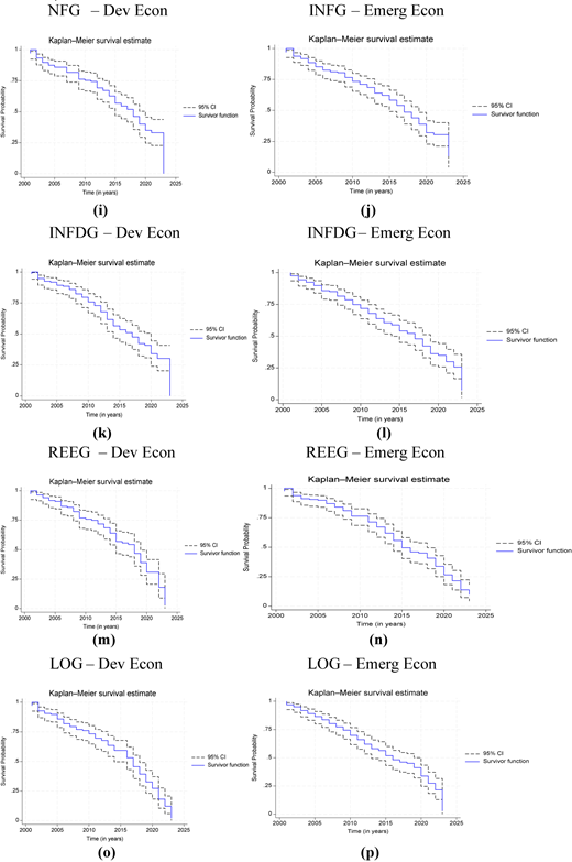
Kaplan–Meier: macroeconomic level. Source(s): Authors’ own work
Sixteen Kaplan–Meier survival plots are arranged in a four-by-four grid, labeled from (a) to (p). Each panel presents a “Kaplan–Meier survival estimate” with a solid step line labeled “Survivor function” and dashed lines labeled “95 percent C I”. In all panels, the horizontal axis is labeled “Time (in years)” and spans from 2000 to 2025 in increments of 5 years, while the vertical axis is labeled “Survival Probability” and ranges from 0 to 1 in increments of 0.25 units. Across all graphs, the survivor function begins near 1.0 at the start of the time axis and declines stepwise over time, with the dashed confidence interval bands surrounding the curve and slightly widening toward later years. Top row: (a) “T G D P G – Dev Econ” shows a steady downward survival trend from near 1.0 around 2000 to low values by about 2023–2025, with narrow confidence bands early and slightly wider bands later. (b) “T G D P G – Emerg Econ” shows a similar gradual stepwise decline over time with comparable confidence interval behavior. Second row: (c) “G D P C G – Dev Econ” displays a consistent decreasing survival curve with step drops and surrounding dashed confidence limits. (d) “G D P C G – Emerg Econ” shows a similar downward step pattern, with the survivor function declining steadily toward lower survival probabilities by the end of the period. Third row: (e) “G D P G – Dev Econ” presents a survival curve that decreases gradually with slightly larger step drops after the mid-period and widening confidence intervals near later years. (f) “G D P G – Emerg Econ” shows a comparable stepwise decline, ending at low survival probability near the end of the time span. Fourth row: (g) “G D P P G – Dev Econ” shows a steady downward trend, with visible step decreases and a widening confidence band near the end. (h) “G D P P G – Emerg Econ” displays a similar pattern, with survival probability declining in stages toward low values by the final years. Fifth row: (i) “I N F G – Dev Econ” shows a gradual downward stepwise survival trend with confidence bands around the curve. (j) “I N F G – Emerg Econ” presents a similar decreasing pattern across time with slightly widening confidence intervals. Sixth row: (k) “I N F D G – Dev Econ” shows a continuous stepwise decline, ending at lower survival probability near the final years. (l) “I N F D G – Emerg Econ” displays a comparable downward trend with dashed confidence limits surrounding the survivor function. Seventh row: (m) “R E E G – Dev Econ” shows a gradual but steady decline in survival probability, with the confidence band widening slightly toward later periods. (n) “R E E G – Emerg Econ” shows a similar downward step pattern with a consistent decline across time. Eighth row: (o) “L O G – Dev Econ” presents a decreasing survivor function with noticeable step drops in later years and surrounding dashed confidence limits. (p) “L O G – Emerg Econ” shows a similar pattern of steady decline toward low survival probability by the end of the time span.Kaplan–Meier: macroeconomic level. Source(s): Authors’ own work
Emerging economies must focus on diversification, strengthening institutions and implementing structural reforms to boost stability and resilience. Developed economies maintain higher per capita output (GDPPG) and better inflation control (INFG, INFDG), while emerging markets struggle with income inequality and inflationary pressures, requiring enhanced monetary frameworks and inclusive growth policies.
Exchange rate volatility (REEG) and governance challenges (LOG) are also more pronounced in emerging economies. Improving exchange rate management, legal frameworks and governance structures is crucial for long-term stability and competitiveness in these markets.
The following indicates the Kaplan–Meier macroeconomic level we composite for both developed and emerging economies.
4.3 Cox model
In Table 9, the Cox model results explain how selected liquidity, banking, market and macroeconomic factors shape the hazard of financial failure over time, with clear differences between developed and emerging economies. For developed economies, broad money growth (M3G) has no meaningful effect on financial stability, with a hazard ratio of 0.999 and p-value of 0.994, implying that liquidity shifts are largely absorbed within mature and well-regulated systems. By contrast, NFAG raises the risk of financial instability by 43.1%, with a hazard ratio of 1.431 and p-value of 0.001, pointing to sensitivity to global capital movements even in advanced settings. Deposit interest rates (DIG) and BLRG modestly reduce risk, with hazard ratios of 0.996 and 0.995, respectively, and both are statistically significant, which is consistent with the idea that tighter funding conditions and stronger liquidity buffers can limit fragility.
Cox model for the banking sector
| a) Developed economies | b) Emerging economies | ||
|---|---|---|---|
| Variables | Haz. ratio | Variables | Haz. ratio |
| M3G | 0.9998 | M3G | 1.0067 |
| (0.0157) | (0.0137) | ||
| NFAG | 1.4310*** | NFAG | 1.1909*** |
| (0.1601) | (0.0584) | ||
| LIG | 0.9988 | LIG | 0.9990 |
| (0.0015) | (0.0050) | ||
| BLRG | 0.9949** | BLRG | 0.9722*** |
| (0.0020) | (0.0043) | ||
| DIG | 0.9960** | DIG | 0.9977 |
| (0.0018) | (0.0015) | ||
Note(s): *p-value <0.10, **p-value <0.05, ***p-value <0.001
In emerging economies, M3G again shows no significant effect, while NFAG increases financial instability, suggesting that external balance sheet exposure is a recurring channel of risk. Interest rate movements, captured by DIG and lending interest rates (LIG), are not statistically significant in explaining financial failure. However, BLRG reduces risk, reinforcing the role of liquidity management in crisis prevention. These patterns align with evidence that fast credit and financial expansion can create vulnerabilities and amplify boom bust dynamics, strengthening the case for macroprudential support alongside inflation targeting (Fouejieu, 2017; Borio et al., 2023; Akinci and Olmstead-Rumsey, 2018).
Turning to market indicators in Table 10, developed economies show hazard ratios for MCG and STG that are close to 1 with non-significant p-values. This suggests that fluctuations in equity market size and trading activity do not meaningfully change the hazard of market failure, which fits the view that regulatory depth, liquidity and diversified financial structures help absorb market swings. In emerging economies, hazard ratios for MCG and STG exceed 1 and are statistically significant, indicating that faster market expansion and higher trading growth are associated with greater instability risk. This result reflects weaker market infrastructure, thinner liquidity and higher exposure to external shocks, and it is consistent with the link between rapid stock price movements, bubble dynamics and fragility in less mature systems (Fouejieu, 2017; Alvarez and Camacho, 2023).
Cox model for the stock market
| a) Developed economies | b) Emerging economies | ||
|---|---|---|---|
| Variables | Haz. ratio | Variables | Haz. ratio |
| MSG | 1.006 | MSG | 1.000 |
| (0.0044) | (0.0028) | ||
| STG | 0.9873*** | STG | 0.9949** |
| (0.0042) | (0.0024) | ||
Note(s): *p-value <0.10, **p-value <0.05, ***p-value <0.001
Table 11 extends the analysis to macroeconomic stability. In developed economies, hazard ratios for trade as a percentage of GDPG (TGDPG), GDPG and inflation dispersion (INFDG) are close to 1 and likely have p-values above 0.05, suggesting limited effects on macroeconomic failure. Lower inflation (INFG) reduces macroeconomic risk with a significant p-value, reinforcing the stabilising role of price discipline. Real effective exchange rate growth (REEG) has a hazard ratio close to 1 with an insignificant p-value, implying minimal additional risk. Emerging economies show hazard ratios above 1 for TGDPG, GDPG, INFG, INFDG and REEG, indicating greater instability linked to trade exposure, growth volatility, inflation pressures and exchange rate swings. This fits the argument that policy coordination and institutional strength raise resilience in advanced economies, while weaker frameworks leave emerging markets more exposed during stress (Fouejieu, 2017; De Bandt et al., 2024).
Cox model for the macroeconomic level
| a) Developed economies | b) Emerging economies | ||
|---|---|---|---|
| Variable | Haz. ratio | Variable | Haz. ratio |
| TGDPG | 0.9696 | TGDPG | 0.1.009 |
| (0.0201) | (0.0142) | ||
| GDPCG | 0.2065 | GDPCG | 768.5523 |
| (0.7995) | (3318.45) | ||
| GDPG | 1.000 | GDPG | 0.9997 |
| (0.0004) | (0.0001) | ||
| GDPPG | 7.4659 | GDPPG | 0.1516 |
| (12.9854) | (0.2677) | ||
| INFG | 0.9998 | INFG | 0.9984 |
| (0.0007) | (0.0009) | ||
| INFDG | 0.9999 | INFDG | 0.9970 |
| (0.0002) | (0.0017) | ||
| REEG | 1.0409 | REEG | 0.9720 |
| (0.0277) | (0.0174) | ||
| LOG | 0.9140 | LOG | 0.9987 |
| (0.1881) | (0.0003) | ||
Note(s): *p-value <0.10, **p-value <0.05, ***p-value <0.001
4.4 Robust check
A robustness check was conducted to examine whether the relationship between inflation targeting and financial stability changes over time. Specifically, we focused on the period from 2001 to 2018 (pre-COVID-19) and compared it to the full dataset covering 2001–2023, which includes post-COVID-19 data. Analysing these two distinct periods to assess if the pandemic altered the dynamics between inflation targeting and financial stability, providing valuable insights into the adaptability and resilience of inflation-targeting frameworks during economic disruptions. The robustness check is essential for validating the consistency of our findings, ensuring they are not skewed by specific time frames or anomalies like the COVID-19 shock. Consistent results across periods suggest a stable impact of inflation targeting on financial stability. However, significant differences may indicate a need for policymakers to adapt inflation-targeting strategies in response to recent challenges. Tables 12–14 show the robust test results for the banking sector, stock market and macroeconomic level, respectively.
Robust tests for the banking sector
| Variables | Haz. ratio | Variables | Haz. ratio |
|---|---|---|---|
| M3G | 0.9840 | M3G | 0.9737 |
| (0.0128) | (0.1173) | ||
| NFAG | 1.7852** | NFAG | 1.1271* |
| (0.2151) | (0.0549) | ||
| LIG | 0.9116 | LIG | 0.9927 |
| (0.0055) | (0.0074) | ||
| BLRG | 0.9987*** | BLRG | 1.0013** |
| (0.0025) | (0.0004) | ||
| DIG | 0.9992 | DIG | 0.9929** |
| (0.0030) | (0.0040) |
Note(s): *p-value <0.05, **p-value <0.01, ***p-value <0.001
Robust tests for the stock market
| (a) Developed economics | (b) Emerging economics | ||
|---|---|---|---|
| Variables | Haz. ratio | Variables | Haz. ratio |
| MCG | 1.0063 | MCG | 1.0009 |
| (0.0026) | (0.0021) | ||
| STG | 0.9995*** | STG | 1.0014** |
| (0.0035) | (0.0016) | ||
Note(s): *p-value<0.10, **p-value<0.05, ***p-value<0.001
Robust tests for the macroeconomic level
| a) Developed economics | b) Emerging economics | ||
|---|---|---|---|
| Variables | Haz. ratio | Variables | Haz. ratio |
| TGDPG | 0.9647 | TGDPG | 1.0024 |
| (0.0191) | (0.0101) | ||
| GDPCG | 0.1114 | GDPCG | 15.3479 |
| (0.7559) | (59.9218) | ||
| GDPG | 1.00005 | GDPG | 0.9900 |
| (0.0001) | (0.0001) | ||
| GDPPG | 10.2871 | GDPPG | 0.0523 |
| (21.2181) | (0.1295) | ||
| INFG | 1.0001 | INFG | 0.9900 |
| (0.0005) | (0.0006) | ||
| INFDG | 1.0002 | INFDG | 0.9890 |
| (0.0001) | (0.0005) | ||
| REEG | 1.0480 | REEG | 0.9968 |
| (0.0206) | (0.0125) | ||
| LOG | 1.0059 | LOG | 1.0323 |
| (0.0239) | (0.0003) | ||
The robustness strategy follows three steps. First, we compare non-parametric life table and Kaplan–Meier survival functions with semi-parametric Cox proportional hazard estimates for the banking sector, stock market and macroeconomic level. The close correspondence between the sector-specific survival profiles and the estimated hazard ratios indicates that the main patterns are not driven by the functional form of the model and are robust across estimation methods. Second, we re-estimate the Cox models on an alternative sample that excludes the COVID-19 period (2001–2018) and contrast the results with those obtained for the full sample (2001–2023). The pre-COVID robustness checks reported in Tables 12–14 show that key covariates, such as liquidity conditions, net foreign assets and interest rates, retain the same sign and remain statistically significant for both developed and emerging economies, even though the magnitude of some coefficients changes. This stability suggests that the main conclusions do not depend on the inclusion of the COVID-19 shock. Third, we examine whether robustness holds across country groups by comparing hazard ratios for developed and emerging economies separately. For the banking sector and macroeconomic level, the hazard ratios remain above or close to one in both the baseline and robustness specifications, confirming that these variables are systematically associated with higher risks of financial instability, while stock-market volatility is more destabilising in emerging markets. Overall, the convergence of results across alternative estimation methods, time windows and country groups strengthens the credibility of the empirical findings.
4.5 Conclusions
This study evaluates the effectiveness of inflation-targeting monetary policies in promoting financial stability in developed and emerging economies. Using survival analysis, including Kaplan–Meier and Cox proportional hazards models, it compares financial stability across both groups and examines how macroeconomic, stock market and banking-sector factors shape financial outcomes.
The study reveals differences between developed and emerging economies. In developed economies, inflation targeting effectively maintains financial stability reflecting robust macroeconomic structures, well-established financial systems and stronger institutions. These economies show longer survival periods of financial stability, successfully managing inflation and financial risks.
Emerging economies experience shorter durations of financial stability and greater vulnerability to external shocks, including volatile capital flows and currency fluctuations. Weaker institutions and banking systems contribute to earlier failure of financial stability. While inflation targeting supports price stability, it does not uniformly ensure financial stability in these regions. Emerging markets may need additional macroprudential measures to address financial imbalances.
The study indicates that developed-economy central banks manage financial risks more effectively, supporting longer financial stability under inflation targeting. In contrast, emerging economies display weaker responses to financial imbalances and remain more vulnerable to external shocks, credit expansion and exchange rate volatility.
Ultimately, while inflation targeting supports price stability, its contribution to financial stability is contingent on institutional and economic conditions with emerging economies requiring complementary macroprudential measures and institutional reforms to limit financial vulnerabilities.
4.6 Policy recommendations
The findings have important policy implications, particularly for emerging markets. These economies should strengthen their macroprudential policies by integrating stricter capital requirements, credit controls and LTV ratios to kerb financial vulnerabilities. Such measures enhance financial system resilience and reduce crisis risk. For example, stricter LTV ratios can limit housing market booms, while enhanced capital requirements ensure that financial institutions have enough reserves to weather market stress. These recommendations follow directly from the empirical result that liquidity and credit-related variables exhibit hazard ratios above one for emerging economies, indicating that looser funding conditions and rapid balance sheet expansion are associated with shorter durations of financial stability.
The study underscores the importance of institutional reforms in emerging economies. Stronger legal frameworks, better regulatory oversight and improved governance can reduce financial fragility and enhance investor confidence. This is consistent with the longer survival times observed for developed economies, where robust institutional and regulatory frameworks appear to dampen the impact of macroeconomic and banking-sector shocks on the hazard of instability.
Emerging economies should adopt more flexible inflation-targeting regimes that explicitly incorporate financial stability as a secondary objective, alongside price stability. Central banks should adjust monetary policy in response to evolving financial conditions through interest rate adjustments and macroprudential instruments, while strengthening coordination between monetary and financial regulation to manage risks from volatile capital flows and asset price inflation. The divergence in survival probabilities between developed and emerging economies in our Kaplan–Meier estimates suggests that regimes focussing narrowly on inflation, without complementary macroprudential coordination, are less effective at sustaining financial stability when exposed to external shocks.
In developed economies, although inflation-targeting frameworks are effective, policymakers should continue monitoring credit growth and asset prices to prevent financial imbalances. Allowing limited flexibility around inflation targets in response to financial stability concerns may further enhance resilience, while transparency in monetary and financial stability policies remains essential for maintaining public and investor confidence. This recommendation reflects the evidence that, even in developed economies where survival probabilities are higher, banking sector and macroeconomic covariates still carry non-negligible hazard ratios, implying that complacency about financial risks under successful inflation targeting would be misplaced.
4.7 Limitations and future research
While this study offers valuable insights, several limitations remain. Future research could examine the long-term effectiveness of macroprudential measures, particularly in emerging economies, and how they perform during prolonged financial crises. Future researchers could apply causality tests between region adoption and stability to explore potential two-way effects. Additionally, more research is needed on how different monetary tools, like interest rate caps or foreign exchange interventions, interact with inflation-targeting regimes to extend financial stability.
Further research should assess how institutional quality, particularly central bank independence and regulatory strength, conditions the effectiveness of inflation-targeting frameworks in promoting financial stability. In addition, examining the specific challenges faced by small, open economies would refine understanding of inflation-targeting performance across different economic structures.
Authors’ contributions
NN, TK and CSS conceptualised the study idea, drafted the paper, collected data, analysed data, wrote the introduction section, organised the literature review, drafted the methodology section, interpreted the results and provided the discussions, concluded the study with policy implications and organised the reference list. NN, TK and CSS equally proofread, edited and finalised the study.
Ethics approval statement
This study does not contain any studies with human participants or animals performed by the authors.
Consent for publication
This manuscript is an original work produced by the authors. NN, TK and CSS are aware of its content and approve its submission. It is also important to mention that the manuscript has not been published elsewhere in part or in entirety and is not under consideration by another journal. The authors have given consent for this study to be submitted for publication in Journal of Economic Studies.
Thanks to the DSI/NRF/Newton Fund Trilateral Chair in Transformative Innovation, the 4IR and Sustainable Development for its support.
