


Mining tailings can have mineralogy distinct from natural soils due to their anthropogenic nature. However, the effects of mineralogy on the critical state response of tailings have not yet been studied without the influence of grading. The reasons for differences in the critical state line (CSL) shape and position of geomaterials remain unclear, since the effects of gradation, mineralogy, loading type, particle size, shape and fabric are not well understood. Accordingly, this paper focuses on the effect of mineralogy on the CSL of copper tailings by evaluating two silty-sand tailings. Although these geomaterials exhibit similar gradations, they differ substantially in mineralogy. Triaxial compression tests under three degrees of compaction and four effective confining pressure values (ranging from 50 to 400 kPa) were performed and compared to published results under simple shear conditions. One copper tailings presented non-unique CSLs depending on the initial fabric and loading path, while the other exhibited unique CSLs regardless of the initial density or loading condition. The results also revealed the influence of mineralogy on the critical state parameter M, with the micaceous tailings presenting a lower critical state friction angle than the tectosilicate-rich one.
NOTATION
- a
the intercept at 1 kPa of a curved critical state line (CSL) (in the υ−ln p′ space)
- b
the gradient of a curved CSL (in the υ−ln p′ space)
- c
the adjustment exponent of a curved CSL (in the υ−ln p′ space)
- e
void ratio
- Gs
specific gravity
- M
critical state stress ratio (in the p′–q space)
- Mss
critical state stress ratio (in the p′–q space) for simple shear tests
- Mtc
critical state stress ratio (in the p′–q space) for triaxial compression tests
- p′
mean effective stress
- p′0
initial mean effective stress (just before shearing)
- q
deviatoric stress – triaxial test (σ1− σ3)
- qss
deviatoric component of stress – simple shear test
- u
pore water pressure
- w
water content
- Γ
the intercept at 1 kPa of a straight CSL (in the υ−ln p′ space)
- εs
shear strain
- η
stress ratio = q/p′
- θ
Lode’s angle
- λ
gradient of a linear CSL (in the υ−ln p′ space)
- σ′h
effective horizontal stress
- σ′v
effective vertical stress
- σ1, σ3
principal stresses
- τ
shear stress
- υ
specific volume = 1 + e
- ϕ′
effective stress friction angle
- ϕ′cs
critical state friction angle
- ϕ′peak
peak friction angle
- ψ
state parameter
INTRODUCTION
The growing global demand for minerals and metals across all sectors of the economy and industry has been responsible for the increase in annual ore production. However, most mines currently explored worldwide are low-grade ore deposits, particularly those for extraction of base metals, such as gold, silver, copper and nickel, among others. Consequently, the main challenge faced by the mining industry is the management of tailings, by-products from the beneficiation activities. In the coming years, a massive volume of tailings will have to be stored and managed by mining companies (Bowker & Chambers, 2017; Islam & Murakami, 2021).
In this context, tailings dams have been the preferred method for storing tailings for operational and economic reasons. Although tailings dams have been built to ensure that tailings are safely stored, protecting the natural environment from degradation, when they fail, the resulting effects greatly and negatively impact the planet, the economy and people, known as the triple bottom line (Byrne et al., 2018; Islam & Murakami, 2021). Since the frequency of failure of tailings storage facilities (TSFs) has been higher than that of other infrastructure, the research interest in tailings has substantially grown, with the aim of enhancing current knowledge on tailings behaviour and proposing alternatives to the disposal of tailings in conventional dams.
The characteristics of tailings, such as their composition, particle morphology and grading, depend on the characteristics of the parent ore and can be highly variable. Specifically, the mineralogy of the particles can greatly influence the geomaterial’s expected behaviour (Nakata et al., 2001; Nocilla et al., 2019; Zhang et al., 2020; Consoli et al., 2024). For instance, Bolton (1986) demonstrated that the critical state friction angle of quartzitic sands is slightly lower than that of feldspathic sands. In contrast, quartz- and feldspar-originated sand presents higher shear strength than micaceous sands.
Mineralogy also exerts influence on the shape of the critical state line (CSL) in the compression plane (v–log p′). Although the shape and position of the CSL of tailings have usually been related to their grading (e.g. Li & Coop, 2019; Secco et al., 2026), Velten et al. (2025) found that two copper tailings with similar gradings presented curved or linear CSLs related to their composition. In addition, uncommon mineralogy has been associated with the occurrence of ‘transitional’ behaviour (Nocilla et al., 2006, 2019; Coop, 2015). Transitional soils present strong forms of fabric that persist after large strains, ultimately leading to a group of semi-parallel CSLs depending on the initial fabric.
Investigation of the transitional response and the influence of mineralogy on geomaterials’ behaviour has primarily been conducted for triaxial compression conditions. However, the conditions imposed in these geotechnical tests are different from those often found in the field (Wagner et al., 2023). Consequently, there is a lack of data on the geomechanical response of tailings under different types of loading, with a few exceptions of studies using the hollow cylinder (e.g. Sadrekarimi, 2016; Fanni et al., 2024) and the direct simple shear (DSS) (e.g. Riveros & Sadrekarimi, 2021; Karim et al., 2023) apparatuses. It is also important to mention the research conducted by Riemer & Seed (1997), which evaluated the effect of the level of consolidation stress, the drainage conditions and the effective stress path on the apparent position of the steady-state line of loose, saturated sands under triaxial compression and simple shear loadings.
Therefore, this paper addresses the influence of mineralogy and stress path on the shape, position and uniqueness of the CSL of two silty-sand copper tailings by comparing triaxial compression results with the simple shear data of Velten et al. (2025). The tailings share a similar particle size distribution while each retains distinct mineralogy. Triaxial tests of copper tailings compacted at different initial void ratios were conducted under confining pressures ranging from 50 to 400 kPa to evaluate possible ‘transitional’ response, which can cause severe problems to the stability of TSFs if not properly identified.
EXPERIMENTAL PROGRAMME
The copper tailings used in this study are the same as those used by Velten et al. (2025), who conducted undrained simple shear tests. Here, complementary mineralogical and morphological tests were conducted since the focus of the work is the influence of microscale characteristics on the macro scale response. Eighteen monotonic drained compression triaxial tests and 17 monotonic undrained compression triaxial tests were conducted.
Materials
Since this study focuses on evaluating the effect of mineralogy, the tailings are identified as CoT (copper tailings rich in tectosilicates) and CoP (copper tailings rich in phyllosilicates), referring to the different minerals they present. Fig. 1 shows the grain size distribution of both tailings and pictures of samples for the simple shear and triaxial tests of both geomaterials. Table 1 summarises the main physical characteristics of each material.
 The particle-size distribution graph plots percent finer by weight vertically against particle diameter d in millimetres horizontally for C o T and C o P. The horizontal axis uses a logarithmic scale from 0.001 to 1.000 millimetres. The vertical axis ranges from 0 to 100 per cent in intervals of 10 per cent. C o T is marked by open triangles and C o P by filled circles. Both curves increase with particle diameter. C o T rises gradually from about 3 per cent near 0.001 millimetres to about 31 per cent near 0.03 millimetres, 47 per cent near 0.08 millimetres, 57 per cent near 0.10 millimetres, 68 per cent near 0.15 millimetres, 81 per cent near 0.21 millimetres and 92 per cent near 0.30 millimetres, reaching approximately 100 per cent beyond 0.5 millimetres. C o P rises from about 2 per cent near 0.001 millimetres to about 19 per cent near 0.03 millimetres, then increases more steeply through about 35 per cent near 0.06 millimetres, 42 per cent near 0.08 millimetres, 70 per cent near 0.11 millimetres, 88 per cent near 0.15 millimetres and 97 per cent near 0.21 millimetres, reaching approximately 100 per cent near 0.3 millimetres. Embedded views associated with the curves contain cylindrical specimens of different proportions, loose granular material and compact cylindrical material samples.
Particle size distribution of the total copper tailings samples
The particle-size distribution graph plots percent finer by weight vertically against particle diameter d in millimetres horizontally for C o T and C o P. The horizontal axis uses a logarithmic scale from 0.001 to 1.000 millimetres. The vertical axis ranges from 0 to 100 per cent in intervals of 10 per cent. C o T is marked by open triangles and C o P by filled circles. Both curves increase with particle diameter. C o T rises gradually from about 3 per cent near 0.001 millimetres to about 31 per cent near 0.03 millimetres, 47 per cent near 0.08 millimetres, 57 per cent near 0.10 millimetres, 68 per cent near 0.15 millimetres, 81 per cent near 0.21 millimetres and 92 per cent near 0.30 millimetres, reaching approximately 100 per cent beyond 0.5 millimetres. C o P rises from about 2 per cent near 0.001 millimetres to about 19 per cent near 0.03 millimetres, then increases more steeply through about 35 per cent near 0.06 millimetres, 42 per cent near 0.08 millimetres, 70 per cent near 0.11 millimetres, 88 per cent near 0.15 millimetres and 97 per cent near 0.21 millimetres, reaching approximately 100 per cent near 0.3 millimetres. Embedded views associated with the curves contain cylindrical specimens of different proportions, loose granular material and compact cylindrical material samples.Particle size distribution of the total copper tailings samples
Physical properties of copper tailings
| Parameters | CoT | CoP |
|---|---|---|
| Total tailings | Total tailings | |
| Specific gravity, Gs | 2·814 | 3·149 |
| Gravel: % | 0·00 | 0·00 |
| Coarse sand: % | 0·00 | 0·00 |
| Medium sand: % | 1·55 | 0·00 |
| Fine sand: % | 50·98 | 57·70 |
| Total sand: % | 52·53 | 57·70 |
| Silt: % | 37·44 | 33·70 |
| Clay: % | 10·03 | 8·60 |
| Mean particle size, D50: mm | 0·082 | 0·082 |
| Uniformity coefficient, Cu | 26·7 | 15·9 |
| Coefficient of curvature, Ccr | 1·7 | 5·1 |
| LL: % | — | — |
| IP: % | Non-plastic | Non-plastic |
| ASTM – USCS classification | SM | SM |
| Standard Proctor optimum moisture content, wopt: % | 12·76 | 14·43 |
| Standard Proctor maximum dry density, γdmax: kN/m3 | 18·49 | 19·02 |
| Modified Proctor optimum moisture content, wopt: % | 10·40 | 10·25 |
| Modified Proctor maximum dry density, γdmax: kN/m3 | 19·44 | 21·13 |
| Maximum void ratio: emax | 1·479 | 2·044 |
| Minimum void ratio: emin | 0·420 | 0·462 |
The particle size distribution was obtained by way of sieve and sedimentation analysis according to ASTM D6913 (ASTM, 2017a) and ASTM D7928 (ASTM, 2021a), respectively. The specific gravity was assessed following the ASTM D854 (ASTM, 2014) procedures, and the Atterberg limits were evaluated according to ASTM D4318 (ASTM, 2017b). Both tailings are silty sands (SM), according to the Unified Soil Classification System (ASTM, 2017c). Also, they are classified as well-graded materials (Cu > 5) and present similar gradings with an identical D50.
Figure 2 displays the compaction curves at standard (ASTM, 2021b) and modified (ASTM, 2021c) efforts, in terms of the void ratios of both tailings, which clearly offer some insight into the arrangements and fabric produced when compacting different materials (Wagner et al., 2025). From Fig. 2, the difference between the modified and the normal minimum void ratio obtained for each optimum water content is close to 0·16 for CoP and 0·07 for CoT. This result can be attributed to differences in the packing of grains, since CoT exhibits bulky particles and CoP flat ones, as will be discussed below. The lower void ratio of CoT does not represent a denser state, however, which can be further confirmed by the similar relative density values (93% for CoT at the optimum compaction point for standard energy and 90% for CoP under the same conditions).
 The line graph plots void ratio e vertically from 0.3 to 1.0 in intervals of 0.1 against moisture content w in per cent horizontally from 4 to 20. The legend identifies C o T Standard Proctor with solid lines and cross markers, C o T Modified Proctor with dotted lines and cross markers, C o P Standard Proctor with solid lines and diamond markers, and C o P Modified Proctor with dotted lines and diamond markers. C o T Standard Proctor decreases from about 0.58 at roughly 9.7 per cent moisture content to a minimum near 0.49 at about 12.8 per cent, then increases to about 0.58 near 16.8 per cent. C o T Modified Proctor decreases from about 0.51 near 4.6 per cent to about 0.42 near 10.4 per cent, then increases to about 0.51 near 14.2 per cent. C o P Standard Proctor decreases from about 0.86 near 8 per cent to about 0.62 near 14.4 per cent, then increases to about 0.73 near 18.4 per cent. C o P Modified Proctor decreases from about 0.54 near 8.2 per cent to a minimum near 0.46 around 10.3 per cent, then rises to about 0.62 near 14.1 per cent.
Compaction characteristics of copper tailings samples. Compaction curves in terms of void ratio
The line graph plots void ratio e vertically from 0.3 to 1.0 in intervals of 0.1 against moisture content w in per cent horizontally from 4 to 20. The legend identifies C o T Standard Proctor with solid lines and cross markers, C o T Modified Proctor with dotted lines and cross markers, C o P Standard Proctor with solid lines and diamond markers, and C o P Modified Proctor with dotted lines and diamond markers. C o T Standard Proctor decreases from about 0.58 at roughly 9.7 per cent moisture content to a minimum near 0.49 at about 12.8 per cent, then increases to about 0.58 near 16.8 per cent. C o T Modified Proctor decreases from about 0.51 near 4.6 per cent to about 0.42 near 10.4 per cent, then increases to about 0.51 near 14.2 per cent. C o P Standard Proctor decreases from about 0.86 near 8 per cent to about 0.62 near 14.4 per cent, then increases to about 0.73 near 18.4 per cent. C o P Modified Proctor decreases from about 0.54 near 8.2 per cent to a minimum near 0.46 around 10.3 per cent, then rises to about 0.62 near 14.1 per cent.Compaction characteristics of copper tailings samples. Compaction curves in terms of void ratio
Mineralogical and morphological aspects
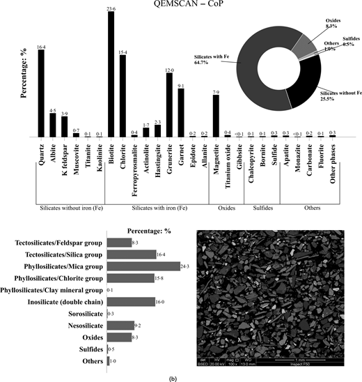
Figure 3 presents the quantitative determination of minerals in both copper tailings studied and their scanning electron microscopy (SEM) analysis. The qualitative evaluation of minerals by scanning electron microscopy (QEMSCAN) method was adopted for this purpose, which is based on SEM analysis and a mineral database. This analysis verified that CoT is constituted mainly by tectosilicates (17·9% quartz and 36·7% albite/feldspar, totalling 54·6%). In turn, CoP is composed of tectosilicates (16·4% quartz and 8·3% albite/feldspar, totalling 24·7%) and phyllosilicates (24·3% biotite – mica group – and 15·8% chlorite – chlorite group, totalling 40·1%).
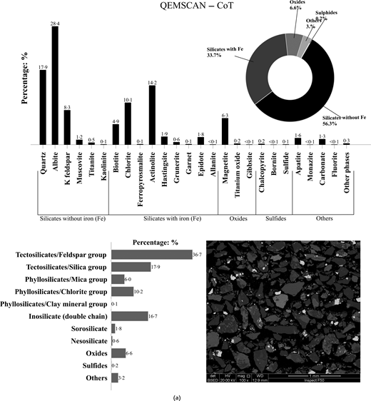
Qualitative and quantitative mineralogical analysis using QEMSCAN technique, with grains morphology from SEM analysis: (a) CoT – minerals detected from darkest to lightest grey tone: quartz, albite, K feldspar, scapolite, actinolite, biotite, hastingsite, magnetite and chalcopyrite; and (b) CoP – minerals detected from darkest to lightest grey tone: quartz, biotite, garnet, magnetite and sulfides
Qualitative and quantitative mineralogical analysis using QEMSCAN technique, with grains morphology from SEM analysis: (a) CoT – minerals detected from darkest to lightest grey tone: quartz, albite, K feldspar, scapolite, actinolite, biotite, hastingsite, magnetite and chalcopyrite; and (b) CoP – minerals detected from darkest to lightest grey tone: quartz, biotite, garnet, magnetite and sulfides
Geologically, the two tailings differ due to the formation processes of their parent rocks. On the one hand, CoT derives from the beneficiation of copper ore bodies encountered in a shear zone established in the contact between metavolcanic sedimentary units and trondhjemitic and tonalitic gneisses. On the other hand, CoP is the by-product of the processing of ore bodies that derive from foliated (or shale aspects) rocks (Teixeira & Lindenmayer, 2012).
As can be seen in Fig. 3, CoT mainly consists of bulky particles with some flocs around, typical of tectosilicates, while CoP presents flocculent (foliated) particles, typical of phyllosilicates, with some flocs bridging bulky particles (Chang et al., 2011). Also, CoP presents biotite particles forming, ordering, bridging and pore-filling microstructures, in agreement with the schematic representations of the microstructure of mica mixed with classical and residual soils proposed by Zhang et al. (2024).
Methods
Moulding of specimens
The testing specimens were moulded considering three different degrees of compaction (i.e. 86, 91 and 95%) established based on the compaction characteristics (Fig. 2) of standard Proctor effort, which is the most common compaction energy adopted in earthworks, especially for mining geotechnical structures. The standard optimum moisture content was used for both tailings regardless of degree of compaction (wop = 12·76% for CoT and wop = 14·43% for CoP). For CoT tailings, the moulding void ratio values were 0·736 (86S), 0·641 (91S) and 0·572 (95S); for CoP tailings, 0·889 (86S), 0·785 (91S) and 0·710 (95S), in which 86, 91 and 95 represent the three different degrees of compaction adopted and ‘S’ means standard, referring to standard Proctor compaction effort. The moist tamping technique (e.g. Frost & Park, 2003; Corrêa & Oliveira Filho, 2019) was used to prepare the specimens for all tests.
For simple shear tests, the specimens’ dimensions, moulding procedures and test specifications are presented in Velten et al. (2025) and are omitted here for the sake of brevity. For triaxial compression tests, moist tailings layers were deposited inside a split mould and manually tamped to the assigned specific volume following the undercompaction method (Ladd, 1978). Three layers were used in this process, with the tops of the first and second layers scarified to guarantee better adherence to the subsequent layer. Figs 4(a) and 4(b) present photographs of dense specimens of CoT (presenting strain localisation) and CoP, respectively, at the end of drained triaxial compression tests under an effective confining pressure of 50 kPa. From those pictures, the uniformity of specimens moulded for the test can be verified. The continuous line represents the location of the base and top of the specimen, and the dashed line represents the location of Hall effect sensors glued over the rubber membrane surface.
 Two views, labelled a and b, present a cylindrical specimen mounted vertically within a transparent testing chamber. In view a, the specimen is enclosed by a flexible membrane and extends between upper and lower loading components. A loading rod and cylindrical component contact the top of the specimen. Two continuous horizontal reference lines and two rows of regularly spaced dots encircle the upper and lower portions of the membrane. A broad metal band surrounds the middle of the specimen and is secured with fasteners and clips. Brackets, fittings and projecting arms are attached around this band. Additional fittings and connections are positioned beside the lower portion of the specimen. The specimen assembly stands on a circular metal base within the transparent chamber, with a vertical metal support column beside it. In view b, the specimen is viewed from another side. The upper loading rod and cylindrical component remain positioned above the specimen. Horizontal reference lines and rows of dots again encircles the membrane. The central metal band, fasteners, clips, brackets, and projecting arms are visible from this orientation, together with connections entering from the sides. The lower specimen section extends into the base assembly, with additional fittings and tubing around it. The transparent cylindrical chamber encloses the complete specimen assembly and rests on the circular metal base, with a vertical support column beside the chamber.
Photographs of dense specimens at the end of the drained triaxial compression test at an effective confining pressure of 50 kPa (continuous line indicates the base and top positions of the specimen; dashed line indicates the positions of Hall effect sensors): (a) CoT_D95S_50 kPa and (b) CoP_D95S_50 kPa. Photographs were taken with membrane to preserve water content determination at the end of the test
Two views, labelled a and b, present a cylindrical specimen mounted vertically within a transparent testing chamber. In view a, the specimen is enclosed by a flexible membrane and extends between upper and lower loading components. A loading rod and cylindrical component contact the top of the specimen. Two continuous horizontal reference lines and two rows of regularly spaced dots encircle the upper and lower portions of the membrane. A broad metal band surrounds the middle of the specimen and is secured with fasteners and clips. Brackets, fittings and projecting arms are attached around this band. Additional fittings and connections are positioned beside the lower portion of the specimen. The specimen assembly stands on a circular metal base within the transparent chamber, with a vertical metal support column beside it. In view b, the specimen is viewed from another side. The upper loading rod and cylindrical component remain positioned above the specimen. Horizontal reference lines and rows of dots again encircles the membrane. The central metal band, fasteners, clips, brackets, and projecting arms are visible from this orientation, together with connections entering from the sides. The lower specimen section extends into the base assembly, with additional fittings and tubing around it. The transparent cylindrical chamber encloses the complete specimen assembly and rests on the circular metal base, with a vertical support column beside the chamber.Photographs of dense specimens at the end of the drained triaxial compression test at an effective confining pressure of 50 kPa (continuous line indicates the base and top positions of the specimen; dashed line indicates the positions of Hall effect sensors): (a) CoT_D95S_50 kPa and (b) CoP_D95S_50 kPa. Photographs were taken with membrane to preserve water content determination at the end of the test
It is important to highlight that significant particle breakage is not expected to occur during the moulding process. Velten et al. (2025) have shown that the same tailings used here presented minimal particle breakage during oedometric compression up to stresses much higher than those promoted in the moulding procedure. As discussed by Wagner et al. (2024), particle breakage has been more directly associated with the stress state experienced by the sample than the load frequency, requiring much higher stress to observe a significant change in grading.
Triaxial testing programme
Isotropically consolidated drained (CID) and undrained (CIU) triaxial compression tests were undertaken to assess the geomechanical response of the two compacted copper tailings under confining pressures spanning from 50 to 400 kPa. In total, 35 triaxial compression tests were conducted, considering both materials, and these are summarised in Table 2 (CoT) and Table 3 (CoP). The nomenclature of the tests was given by A_BC_D kPa, in which ‘A’ is the material studied (e.g. CoT or CoP), ‘B’ refers to the type of triaxial compression test (e.g. D for drained test and U for undrained), ‘C’ refers to degree of compaction of the specimen (e.g. 95S) and ‘D’ is the initial effective confining pressure of the test (e.g. 100 kPa).
Summary of triaxial compression test data, CoT
| Test | p′0: kPa | p′peak: kPa | qpeak: kPa | p′cs: kPa | qcs: kPa | ψc | υ0 | υc | υsh |
|---|---|---|---|---|---|---|---|---|---|
| CoT_U86S_100 kPa | 100 | 106. | 110·5 | 3·4 | 4·4 | 0·06 | 1·72 | 1·72 | 1·72 |
| CoT_U86S_200 kPa | 200 | 150·7 | 133·3 | 6·8 | 4·4 | 0·07 | 1·72 | 1·71 | 1·71 |
| CoT_U91S_100 kPa | 100 | 102·8 | 116·8 | 6·5 | 1·9 | 0·03 | 1·65 | 1·64 | 1·64 |
| CoT_U91S_200 kPa | 200 | 199·9 | 221·6 | 35·9 | 39·1 | 0·03 | 1·64 | 1·63 | 1·63 |
| CoT_U91S_400 kPa | 400 | 267·7 | 267·3 | 76·1 | 94·0 | 0·04 | 1·69 | 1·62 | 1·62 |
| CoT_U95S_50 kPa | 50 | 183·6 | 269·3 | 156·3 | 227·5 | −0·01 | 1·58 | 1·58 | 1·58 |
| CoT_U95S_100 kPa | 100 | 317·3 | 457·9 | 240·6 | 352·3 | −0·01 | 1·58 | 1·58 | 1·58 |
| CoT_U95S_200 kPa | 200 | 346·0 | 495·2 | 216·3 | 314·3 | 0·00 | 1·58 | 1·58 | 1·58 |
| CoT_D86S_50 kPa | 50 | 95·6 | 136·8 | 95·0 | 135·6 | 0·05 | 1·72 | 1·72 | 1·66 |
| CoT_D86S_100 kPa | 100 | 188·6 | 264·3 | 187·0 | 259·8 | 0·06 | 1·72 | 1·71 | 1·64 |
| CoT_D86S_400 kPa | 400 | 791·9 | 1169·4 | 786·3 | 1157·4 | 0·08 | 1·71 | 1·70 | 1·59 |
| CoT_D91S_50 kPa | 50 | 99·6 | 149·5 | 98·3 | 144·7 | 0·03 | 1·65 | 1·65 | 1·61 |
| CoT_D91S_100 kPa | 100 | 204·4 | 307·3 | 200·4 | 297·4 | 0·02 | 1·65 | 1·64 | 1·60 |
| CoT_D91S_400 kPa | 400 | 786·6 | 1159·2 | 771·1 | 1110·5 | 0·04 | 1·65 | 1·63 | 1·57 |
| CoT_D95S_50 kPa | 50 | 99·8 | 150·8 | 93·5 | 132·1 | −0·01 | 1·58 | 1·58 | 1·59 |
| CoT_D95S_100 kPa | 100 | 192·3 | 274·9 | 190·2 | 266·9 | −0·01 | 1·58 | 1·58 | 1·58 |
| CoT_D95S_400 kPa | 400 | 781·2 | 1143·2 | 767·9 | 1103·9 | 0·00 | 1·58 | 1·57 | 1·55 |
Summary of triaxial compression test data, CoP
| Test | p′0: kPa | p′peak: kPa | qpeak: kPa | p′cs: kPa | qcs: kPa | ψc | υ0 | υc | υsh |
|---|---|---|---|---|---|---|---|---|---|
| CoP_U86S_50 kPa | 50 | 39·1 | 41·5 | 13·7 | 26·4 | 0·09 | 1·87 | 1·85 | 1·85 |
| CoP_U86S_100 kPa | 100 | 71·6 | 89·5 | 36·1 | 68·4 | 0·08 | 1·84 | 1·80 | 1·80 |
| CoP_U86S_200 kPa | 200 | 115·3 | 129·8 | 63·4 | 100·0 | 0·09 | 1·88 | 1·75 | 1·75 |
| CoP_U91S_100 kPa | 100 | 69·3 | 84·4 | 44·0 | 67·7 | 0·04 | 1·78 | 1·75 | 1·75 |
| CoP_U91S_200 kPa | 200 | 124·3 | 164·4 | 90·4 | 136·9 | 0·05 | 1·76 | 1·71 | 1·71 |
| CoP_U91S_400 kPa | 400 | 222·0 | 280·0 | 168·2 | 238·3 | 0·06 | 1·76 | 1·68 | 1·68 |
| CoP_U95S_50 kPa | 50 | 104·5 | 154·7 | 104·2 | 154·5 | −0·05 | 1·71 | 1·71 | 1·71 |
| CoP_U95S_100 kPa | 100 | 134·7 | 195·4 | 127·9 | 183·0 | −0·02 | 1·70 | 1·69 | 1·69 |
| CoP_U95S_200 kPa | 200 | 172·2 | 241·6 | 172·2 | 241·6 | 0·01 | 1·69 | 1·67 | 1·67 |
| CoP_D86S_50 kPa | 50 | 91·6 | 125·7 | 90·9 | 123·0 | 0·09 | 1·87 | 1·85 | 1·74 |
| CoP_D86S_100 kPa | 100 | 196·2 | 290·5 | 196·4 | 290·2 | 0·09 | 1·85 | 1·80 | 1·70 |
| CoP_D86S_400 kPa | 400 | 735·1 | 1002·8 | 732·1 | 995·7 | 0·09 | 1·87 | 1·71 | 1·59 |
| CoP_D91S_50 kPa | 50 | 89·4 | 118·1 | 89·4 | 118·1 | 0·01 | 1·77 | 1·77 | 1·72 |
| CoP_D91S_100 kPa | 100 | 191·0 | 272·6 | 190·7 | 272·2 | 0·04 | 1·82 | 1·75 | 1·65 |
| CoP_D91S_400 kPa | 400 | 767·5 | 1100·3 | 766·7 | 1096·2 | 0·06 | 1·83 | 1·67 | 1·55 |
| CoP_D95S_50 kPa | 50 | 94·3 | 130·3 | 92·4 | 125·5 | −0·05 | 1·71 | 1·71 | 1·70 |
| CoP_D95S_100 kPa | 100 | 191·9 | 274·5 | 187·3 | 261·5 | −0·02 | 1·70 | 1·70 | 1·68 |
| CoP_D95S_400 kPa | 400 | 748·5 | 1038·7 | 741·0 | 1021·7 | 0·02 | 1·69 | 1·63 | 1·56 |
The tests followed the recommendations of ASTM D7181 (ASTM, 2020a) and ASTM D4767 (ASTM, 2020b) standards. First, the specimens were submitted to a saturation process composed of carbon dioxide percolation, water percolation and incrementally increasing backpressure to achieve 400 kPa (keeping the mean effective stress equal to 20 kPa). Skempton B values were measured after saturation and were all greater than 0·98. Then, the consolidation phase was conducted by incrementing the chamber pressure up to the desired value.
Finally, the shearing phase was carried out using a strain-controlled method with a rate of 4·32 mm/h for both tests (e.g. CID and CIU) to guarantee a better stress distribution inside the specimen. Also, two Hall effect sensors were used to evaluate the axial displacements, and one was employed to measure the radial displacements (Clayton & Khatrush, 1986). These sensors were fundamental to calculating axial and radial displacements in all stages of the test. The specimen’s dimensions and moisture content at the end of the test were measured, aiming to obtain the void ratio through the most independent forms as possible (Shipton & Coop, 2015). Although end-of-test soil freezing (Reid et al., 2021; Sladen & Handford, 1987) was not used, the measurement of the final moisture content of saturated samples has demonstrated good agreement and sufficient accuracy (Murthy et al., 2007; Shipton & Coop, 2015), particularly when used in conjunction with internal measurements.
RESULTS AND DISCUSSION
Influence of mineralogy on the triaxial compression response of copper tailings
Tables 2 and 3 summarise the main characteristics of undrained and drained triaxial compression tests on CoT and CoP tailings, respectively. Fig. 5(a) (drained monotonic triaxial compression tests) and Fig. 5(b) (undrained monotonic triaxial compression tests) present the results on CoT and CoP tailings.
 Three panels, labelled a, b and c, present stress, volumetric strain, excess pore pressure and dilatancy responses for C o T and C o P tests. Panel a contains two graphs against axial strain epsilon sub a in per cent, extending from 0 to about 22 per cent. The upper graph plots deviatoric stress q in kilopascals from 0 to 1,200. The curves represent C o T D 86 S at 50, 100 and 400 kilopascals, C o T D 91 S at 50 kilopascals, C o T D 95 S at 50 kilopascals, C o P D 86 S at 50, 100 and 400 kilopascals, C o P D 91 S at 50 kilopascals and C o P D 95 S at 50 kilopascals. The two 400 kilopascal D 86 S curves increase strongly throughout the test, reaching approximately 1,160 and 1,000 kilopascals near 18 to 20 per cent axial strain. Curves at intermediate levels rise to approximately 200 to 290 kilopascals. The remaining curves rise rapidly at low axial strain and then remain mainly around 80 to 150 kilopascals, with small fluctuations. The lower graph in panel a plots volumetric strain epsilon sub v in per cent against the same axial-strain range. Its vertical axis extends from negative 1 per cent at the top to 10 per cent at the bottom, with labelled intervals of 1 per cent. One curve moves slightly into negative volumetric strain and remains near negative 0.5 per cent. The other curves move towards increasing positive volumetric strain with axial strain. Their final values range from approximately 0.6 to 6.7 per cent, with the largest responses extending beyond 6 per cent near 18 to 20 per cent axial strain. The legend below this graph identifies the same 10 D-series datasets used in the upper graph. Panel b contains two graphs against axial strain epsilon sub a in per cent, again extending from 0 to about 22 per cent. The upper graph plots deviatoric stress q from 0 to 500 kilopascals in intervals of 50 kilopascals. One response rises steeply to approximately 450 kilopascals at low axial strain, fluctuates between approximately 330 and 430 kilopascals through the early and middle strain range, and then remains around 350 to 370 kilopascals. A second response rises rapidly to approximately 180 to 190 kilopascals and remains close to this level. Other curves initially reach approximately 80 to 130 kilopascals. Some subsequently decline progressively towards approximately zero to 20 kilopascals, while others stabilise around approximately 65 to 110 kilopascals. A lower response rises to approximately 40 kilopascals and then remains near 25 to 30 kilopascals. The lower graph in panel b plots excess pore pressure delta U in kilopascals against axial strain. Its vertical axis is arranged from negative 100 kilopascals at the top through 0 to 400 kilopascals at the bottom, with labelled intervals of 50 kilopascals. The legend identifies C o T U 86 S at 100 and 200 kilopascals, C o T U 91 S at 100 kilopascals, C o T U 95 S at 100 kilopascals, C o P U 86 S at 50, 100 and 200 kilopascals, C o P U 91 S at 100 kilopascals and C o P U 95 S at 100 kilopascals. One curve initially reaches approximately negative 70 kilopascals and then gradually approaches approximately negative 25 kilopascals. Two relatively low positive responses remain around 30 to 45 kilopascals. Several curves increase rapidly towards approximately 60 to 100 kilopascals and then change gradually. The two largest positive responses increase steeply and level near approximately 170 and 190 kilopascals. Panel c plots q over M p prime vertically from 0 to 1.2, in intervals of 0.2, against dilatancy D horizontally from negative 1.0 to 3.0, in intervals of 0.5. The legend identifies C o T D 86 S at 50, 100 and 400 kilopascals, C o T D 91 S at 50 kilopascals, C o T D 95 S at 50 kilopascals, C o P D 86 S at 50, 100 and 400 kilopascals, C o P D 91 S at 50 kilopascals and C o P D 95 S at 50 kilopascals. The datasets are represented by square, circle and triangle markers and by solid, dashed and dotted paths. Many observations cluster near q over M p prime values of approximately 0.7 to 1.0 and dilatancy values from about negative 0.5 to 0.5. Several paths extend towards positive dilatancy between approximately 0.5 and 1.2 as q over M p prime decreases towards approximately 0.2 to 0.7. A group of triangular points extends farther to approximately 2.2 dilatancy, with q over M p prime values decreasing to about 0.1 to 0.4. An open circular reference marker lies at approximately D equals 0 and q over M p prime equals 1. The accompanying annotation gives theta equals 0.00 degrees, M superscript C o T equals 1.46 and M superscript C o P equals 1.40.
CoT and CoP triaxial compression tests: (a) drained tests – D: deviatoric stress–axial strain–volumetric strain; (b) undrained tests – U: deviatoric stress–axial strain–excess pore pressure; and (c) dilatancy, D–(η/ΜCoT and η/ΜCoP)
Three panels, labelled a, b and c, present stress, volumetric strain, excess pore pressure and dilatancy responses for C o T and C o P tests. Panel a contains two graphs against axial strain epsilon sub a in per cent, extending from 0 to about 22 per cent. The upper graph plots deviatoric stress q in kilopascals from 0 to 1,200. The curves represent C o T D 86 S at 50, 100 and 400 kilopascals, C o T D 91 S at 50 kilopascals, C o T D 95 S at 50 kilopascals, C o P D 86 S at 50, 100 and 400 kilopascals, C o P D 91 S at 50 kilopascals and C o P D 95 S at 50 kilopascals. The two 400 kilopascal D 86 S curves increase strongly throughout the test, reaching approximately 1,160 and 1,000 kilopascals near 18 to 20 per cent axial strain. Curves at intermediate levels rise to approximately 200 to 290 kilopascals. The remaining curves rise rapidly at low axial strain and then remain mainly around 80 to 150 kilopascals, with small fluctuations. The lower graph in panel a plots volumetric strain epsilon sub v in per cent against the same axial-strain range. Its vertical axis extends from negative 1 per cent at the top to 10 per cent at the bottom, with labelled intervals of 1 per cent. One curve moves slightly into negative volumetric strain and remains near negative 0.5 per cent. The other curves move towards increasing positive volumetric strain with axial strain. Their final values range from approximately 0.6 to 6.7 per cent, with the largest responses extending beyond 6 per cent near 18 to 20 per cent axial strain. The legend below this graph identifies the same 10 D-series datasets used in the upper graph. Panel b contains two graphs against axial strain epsilon sub a in per cent, again extending from 0 to about 22 per cent. The upper graph plots deviatoric stress q from 0 to 500 kilopascals in intervals of 50 kilopascals. One response rises steeply to approximately 450 kilopascals at low axial strain, fluctuates between approximately 330 and 430 kilopascals through the early and middle strain range, and then remains around 350 to 370 kilopascals. A second response rises rapidly to approximately 180 to 190 kilopascals and remains close to this level. Other curves initially reach approximately 80 to 130 kilopascals. Some subsequently decline progressively towards approximately zero to 20 kilopascals, while others stabilise around approximately 65 to 110 kilopascals. A lower response rises to approximately 40 kilopascals and then remains near 25 to 30 kilopascals. The lower graph in panel b plots excess pore pressure delta U in kilopascals against axial strain. Its vertical axis is arranged from negative 100 kilopascals at the top through 0 to 400 kilopascals at the bottom, with labelled intervals of 50 kilopascals. The legend identifies C o T U 86 S at 100 and 200 kilopascals, C o T U 91 S at 100 kilopascals, C o T U 95 S at 100 kilopascals, C o P U 86 S at 50, 100 and 200 kilopascals, C o P U 91 S at 100 kilopascals and C o P U 95 S at 100 kilopascals. One curve initially reaches approximately negative 70 kilopascals and then gradually approaches approximately negative 25 kilopascals. Two relatively low positive responses remain around 30 to 45 kilopascals. Several curves increase rapidly towards approximately 60 to 100 kilopascals and then change gradually. The two largest positive responses increase steeply and level near approximately 170 and 190 kilopascals. Panel c plots q over M p prime vertically from 0 to 1.2, in intervals of 0.2, against dilatancy D horizontally from negative 1.0 to 3.0, in intervals of 0.5. The legend identifies C o T D 86 S at 50, 100 and 400 kilopascals, C o T D 91 S at 50 kilopascals, C o T D 95 S at 50 kilopascals, C o P D 86 S at 50, 100 and 400 kilopascals, C o P D 91 S at 50 kilopascals and C o P D 95 S at 50 kilopascals. The datasets are represented by square, circle and triangle markers and by solid, dashed and dotted paths. Many observations cluster near q over M p prime values of approximately 0.7 to 1.0 and dilatancy values from about negative 0.5 to 0.5. Several paths extend towards positive dilatancy between approximately 0.5 and 1.2 as q over M p prime decreases towards approximately 0.2 to 0.7. A group of triangular points extends farther to approximately 2.2 dilatancy, with q over M p prime values decreasing to about 0.1 to 0.4. An open circular reference marker lies at approximately D equals 0 and q over M p prime equals 1. The accompanying annotation gives theta equals 0.00 degrees, M superscript C o T equals 1.46 and M superscript C o P equals 1.40.CoT and CoP triaxial compression tests: (a) drained tests – D: deviatoric stress–axial strain–volumetric strain; (b) undrained tests – U: deviatoric stress–axial strain–excess pore pressure; and (c) dilatancy, D–(η/ΜCoT and η/ΜCoP)
Under drained conditions (Fig. 5(a)), both copper tailings presented a strain-hardening response to the end of the test, except for the densest CoT specimen under the lowest confining stress (CoT_D95S_50 kPa), which exhibited the formation of a shear band (see Fig. 4(a)). However, CoT exhibited a stiffer response than CoP. Except for the densest specimen of CoT tailings under the lowest confining stress (CoT_D95S_50 kPa), all tests presented contractive volumetric strains despite their compaction degree. In addition, differences were verified for the M values obtained for CoT (M = 1·46) and for CoP (M = 1·40). Considering that they present similar gradation, the differences observed in M might be associated with their considerable mineralogical differences.
On the undrained geomechanical response (Fig. 5(b)), CoT tailings specimens exhibited a well-defined peak strength followed by a strain-softening response in the deviatoric stress–axial strain diagram. Considerable loss of strength was verified for loose (86S) and medium (91S) states at an effective confining pressure of 100 kPa, indicating the occurrence of static liquefaction. These results are confirmed in the excess pore pressure response for CoT copper tailings (also shown in Fig. 5(b)) – that is, considerable positive excess pore pressure was generated during undrained tests at degrees of compaction of 86% (86S) and 91% (91S). However, negative excess pore pressure values were generated for the densest specimen under 100 kPa (low) confining stress (CoT_U95S_100 kPa). In contrast, CoP tailings specimens presented a ductile response (increasing axial strain, deviatoric stress increased – or kept about constant) with positive pore pressure generation (as also presented in Fig. 5(b)), and undrained instability was not observed. These undrained responses also agree with the monotonic geomechanical response data that Seethalakshmi & Sachan (2020) reported for pure and micaceous sands of Sabarmati soil. In addition, Fig. 5(c) portrays the q/(Mp′)–dilatancy (D) of both tailings, in which M is MCoT (for CoT tailings) or MCoP (for CoP tailings).
Figure 6 compares the response of CoT and CoP tailings presenting similar void ratios initially and prior to shear and under the same confining pressure. Under drained loading conditions, small differences were obtained in the deviatoric stress–axial strain response (Fig. 6(a)), but the CoT specimen presented larger volumetric strains than the CoP specimen. Under undrained loading conditions (Fig. 6(b)), the CoP specimen presented a ductile response, while the CoT specimen liquefied (Fig. 6(b)).
 Two panels, labelled a and b, each contain two graphs comparing C o T and C o P responses. In panel a, the left graph plots deviatoric stress q in kilopascals vertically from 0 to 1,200 against axial strain epsilon sub a horizontally from 0 to 22. The horizontal axis is labelled axial strain epsilon sub a in kilopascals. The legend identifies C o P D 95 S at 50 kilopascals and C o T D 86 S at 50 kilopascals, both with square markers. C o P D 95 S rises rapidly from zero to about 120 kilopascals at low axial strain, then gradually approaches approximately 150 kilopascals and remains nearly level through about 18 per cent axial strain. C o T D 86 S rises rapidly to approximately 80 kilopascals, then increases gradually to around 100 kilopascals by about 8 per cent axial strain, reaches approximately 120 to 130 kilopascals around 10 to 12 per cent and ends near 135 kilopascals at about 19 per cent. The right graph in panel a plots volumetric strain epsilon sub v in per cent vertically against axial strain epsilon sub a in per cent horizontally from 0 to 22, with the horizontal axis placed at the top. The volumetric-strain scale runs from negative 1 at the top through 0 to 7 per cent at the bottom. The legend identifies C o T D 86 S at 50 kilopascals and C o P D 95 S at 50 kilopascals. Both curves begin near zero. C o T D 86 S increases steadily downwards, reaching about 1 per cent near 3 per cent axial strain, 2 per cent near 6 per cent, 3 per cent near 12 per cent and approximately 3.8 per cent near 19 per cent. C o P D 95 S changes much less, reaching approximately 0.3 per cent by about 3 per cent axial strain and gradually increasing to approximately 0.6 per cent near 18 per cent. In panel b, the left graph plots deviatoric stress q in kilopascals vertically from 0 to 500 against axial strain epsilon sub a in per cent horizontally from 0 to 22. The legend identifies C o T U 86 S at 100 kilopascals and C o P U 95 S at 100 kilopascals, both with circular markers. C o P U 95 S rises rapidly to approximately 180 to 190 kilopascals by about 2 to 3 per cent axial strain, remains near 180 to 195 kilopascals with modest fluctuations, and ends near 185 kilopascals at about 19 per cent strain. C o T U 86 S initially reaches approximately 110 kilopascals and then decreases continuously, falling below 50 kilopascals by about 3 per cent axial strain, approaching approximately 10 kilopascals around 7 per cent and remaining close to zero from roughly 10 to 16 per cent. The right graph in panel b plots excess pore pressure delta U in kilopascals vertically against axial strain epsilon sub a, with the horizontal axis labelled in kilopascals and positioned at the top from 0 to 22. The vertical scale runs from negative 100 kilopascals at the top through 0 to 400 kilopascals at the bottom. The legend identifies C o T U 86 S at 100 kilopascals and C o P U 95 S at 100 kilopascals. Both begin near zero. C o T U 86 S increases rapidly to about 50 kilopascals and then more gradually towards approximately 100 kilopascals by about 18 per cent axial strain. C o P U 95 S increases to approximately 30 kilopascals at low axial strain and remains nearly constant around 30 kilopascals through the remainder of the plotted range.
Comparison of CoT and CoP tailings at a same void ratio prior to shearing under (a) drained and (b) undrained triaxial compression loading
Two panels, labelled a and b, each contain two graphs comparing C o T and C o P responses. In panel a, the left graph plots deviatoric stress q in kilopascals vertically from 0 to 1,200 against axial strain epsilon sub a horizontally from 0 to 22. The horizontal axis is labelled axial strain epsilon sub a in kilopascals. The legend identifies C o P D 95 S at 50 kilopascals and C o T D 86 S at 50 kilopascals, both with square markers. C o P D 95 S rises rapidly from zero to about 120 kilopascals at low axial strain, then gradually approaches approximately 150 kilopascals and remains nearly level through about 18 per cent axial strain. C o T D 86 S rises rapidly to approximately 80 kilopascals, then increases gradually to around 100 kilopascals by about 8 per cent axial strain, reaches approximately 120 to 130 kilopascals around 10 to 12 per cent and ends near 135 kilopascals at about 19 per cent. The right graph in panel a plots volumetric strain epsilon sub v in per cent vertically against axial strain epsilon sub a in per cent horizontally from 0 to 22, with the horizontal axis placed at the top. The volumetric-strain scale runs from negative 1 at the top through 0 to 7 per cent at the bottom. The legend identifies C o T D 86 S at 50 kilopascals and C o P D 95 S at 50 kilopascals. Both curves begin near zero. C o T D 86 S increases steadily downwards, reaching about 1 per cent near 3 per cent axial strain, 2 per cent near 6 per cent, 3 per cent near 12 per cent and approximately 3.8 per cent near 19 per cent. C o P D 95 S changes much less, reaching approximately 0.3 per cent by about 3 per cent axial strain and gradually increasing to approximately 0.6 per cent near 18 per cent. In panel b, the left graph plots deviatoric stress q in kilopascals vertically from 0 to 500 against axial strain epsilon sub a in per cent horizontally from 0 to 22. The legend identifies C o T U 86 S at 100 kilopascals and C o P U 95 S at 100 kilopascals, both with circular markers. C o P U 95 S rises rapidly to approximately 180 to 190 kilopascals by about 2 to 3 per cent axial strain, remains near 180 to 195 kilopascals with modest fluctuations, and ends near 185 kilopascals at about 19 per cent strain. C o T U 86 S initially reaches approximately 110 kilopascals and then decreases continuously, falling below 50 kilopascals by about 3 per cent axial strain, approaching approximately 10 kilopascals around 7 per cent and remaining close to zero from roughly 10 to 16 per cent. The right graph in panel b plots excess pore pressure delta U in kilopascals vertically against axial strain epsilon sub a, with the horizontal axis labelled in kilopascals and positioned at the top from 0 to 22. The vertical scale runs from negative 100 kilopascals at the top through 0 to 400 kilopascals at the bottom. The legend identifies C o T U 86 S at 100 kilopascals and C o P U 95 S at 100 kilopascals. Both begin near zero. C o T U 86 S increases rapidly to about 50 kilopascals and then more gradually towards approximately 100 kilopascals by about 18 per cent axial strain. C o P U 95 S increases to approximately 30 kilopascals at low axial strain and remains nearly constant around 30 kilopascals through the remainder of the plotted range.Comparison of CoT and CoP tailings at a same void ratio prior to shearing under (a) drained and (b) undrained triaxial compression loading
Influence of loading direction on the response of copper tailings
Figures 7 and 8 display the stress paths for CoT and CoP tailings, respectively. The end-of-test points are highlighted for each material and for each type of loading studied, and the respective CSLs are also drawn, with the proper inclination: for simple shear loading, M = 1·02 for CoT tailings (Fig. 7(a)) and M = 0·99 for CoP tailings (Fig. 8(a)), while for triaxial compression loading, M = 1·46 for CoT tailings (Fig. 7(b)) and M = 1·40 for CoP (Fig. 8(b)).
 Two graphs, labelled a and b, plot deviatoric stress q in kilopascals vertically against mean effective stress p prime in kilopascals horizontally. In graph a, both axes range from 0 to 450 kilopascals, with major intervals of 50 kilopascals. The legend identifies C o T U 86 S, C o T U 91 S and C o T U 95 S, shearing endpoints marked by filled circles, and a dashed fitted line defined by q equals 1.02 p prime, R squared equals 0.99 and p value less than 0.0001. Multiple curved stress paths occur at increasing stress levels. Lower paths rise to approximately 30 to 60 kilopascals deviatoric stress before returning towards zero. Subsequent paths reach approximately 90, 150 to 170, and 240 to 275 kilopascals before curving downwards. Larger paths extend from around 200 to 400 kilopascals mean effective stress and return towards zero near 400 kilopascals. An upper U 95 S path rises sharply from approximately 260 kilopascals mean effective stress and 270 kilopascals deviatoric stress to a peak near 390 kilopascals deviatoric stress at about 320 kilopascals mean effective stress, then decreases slightly towards a shearing endpoint near 370 kilopascals. Shearing endpoints form an ascending sequence from low stresses through approximately 90, 165, 205 and 240 kilopascals to about 375 kilopascals deviatoric stress. The dashed fitted line rises diagonally through these endpoints from the origin to approximately 410 kilopascals deviatoric stress at 400 kilopascals mean effective stress. In graph b, the horizontal axis ranges from 0 to 800 kilopascals in major intervals of 100 kilopascals, and the vertical axis ranges from 0 to 1,200 kilopascals in major intervals of 100 kilopascals. The legend identifies D 86 S, D 91 S and D 95 S as solid curves and U 86 S, U 91 S and U 95 S as dashed curves. Filled circles mark shearing endpoints. The dashed fitted line is defined by q equals 1.46 p prime, R squared equals 0.99 and p value less than 0.0001. At lower stresses, multiple D and U paths extend between approximately 0 and 300 kilopascals mean effective stress and approximately 0 and 480 kilopascals deviatoric stress. Several paths rise through shearing endpoints along the fitted line, while some U paths curve back towards zero deviatoric stress near approximately 100, 200 and 400 kilopascals mean effective stress. Other paths cluster between approximately 200 and 300 kilopascals mean effective stress and 300 to 480 kilopascals deviatoric stress. At higher stresses, closely overlapping D paths rise almost linearly from approximately 400 kilopascals mean effective stress and zero deviatoric stress to above 1,100 kilopascals deviatoric stress near 780 kilopascals means effective stress. Upper shearing endpoints occur near approximately 1,110 and 1,160 kilopascals deviatoric stress. The dashed fitted line extends diagonally from the origin through the shearing endpoints towards approximately 1,160 kilopascals deviatoric stress near 800 kilopascals mean effective stress.
Stress paths at the p′–q plane for CoT tailings: (a) simple shear tests; (b) triaxial compression tests
Two graphs, labelled a and b, plot deviatoric stress q in kilopascals vertically against mean effective stress p prime in kilopascals horizontally. In graph a, both axes range from 0 to 450 kilopascals, with major intervals of 50 kilopascals. The legend identifies C o T U 86 S, C o T U 91 S and C o T U 95 S, shearing endpoints marked by filled circles, and a dashed fitted line defined by q equals 1.02 p prime, R squared equals 0.99 and p value less than 0.0001. Multiple curved stress paths occur at increasing stress levels. Lower paths rise to approximately 30 to 60 kilopascals deviatoric stress before returning towards zero. Subsequent paths reach approximately 90, 150 to 170, and 240 to 275 kilopascals before curving downwards. Larger paths extend from around 200 to 400 kilopascals mean effective stress and return towards zero near 400 kilopascals. An upper U 95 S path rises sharply from approximately 260 kilopascals mean effective stress and 270 kilopascals deviatoric stress to a peak near 390 kilopascals deviatoric stress at about 320 kilopascals mean effective stress, then decreases slightly towards a shearing endpoint near 370 kilopascals. Shearing endpoints form an ascending sequence from low stresses through approximately 90, 165, 205 and 240 kilopascals to about 375 kilopascals deviatoric stress. The dashed fitted line rises diagonally through these endpoints from the origin to approximately 410 kilopascals deviatoric stress at 400 kilopascals mean effective stress. In graph b, the horizontal axis ranges from 0 to 800 kilopascals in major intervals of 100 kilopascals, and the vertical axis ranges from 0 to 1,200 kilopascals in major intervals of 100 kilopascals. The legend identifies D 86 S, D 91 S and D 95 S as solid curves and U 86 S, U 91 S and U 95 S as dashed curves. Filled circles mark shearing endpoints. The dashed fitted line is defined by q equals 1.46 p prime, R squared equals 0.99 and p value less than 0.0001. At lower stresses, multiple D and U paths extend between approximately 0 and 300 kilopascals mean effective stress and approximately 0 and 480 kilopascals deviatoric stress. Several paths rise through shearing endpoints along the fitted line, while some U paths curve back towards zero deviatoric stress near approximately 100, 200 and 400 kilopascals mean effective stress. Other paths cluster between approximately 200 and 300 kilopascals mean effective stress and 300 to 480 kilopascals deviatoric stress. At higher stresses, closely overlapping D paths rise almost linearly from approximately 400 kilopascals mean effective stress and zero deviatoric stress to above 1,100 kilopascals deviatoric stress near 780 kilopascals means effective stress. Upper shearing endpoints occur near approximately 1,110 and 1,160 kilopascals deviatoric stress. The dashed fitted line extends diagonally from the origin through the shearing endpoints towards approximately 1,160 kilopascals deviatoric stress near 800 kilopascals mean effective stress.Stress paths at the p′–q plane for CoT tailings: (a) simple shear tests; (b) triaxial compression tests
 Two stress-path graphs, labelled a and b, plot deviatoric stress q in kilopascals vertically against mean effective stress p prime in kilopascals horizontally. In graph a, both axes range from 0 to 450 kilopascals, with major intervals of 50 kilopascals. The legend identifies C o P U 86 S, C o P U 91 S and C o P U 95 S, black circular shearing endpoints, and a dashed fitted line labelled q equals 0.999 p prime, R squared equals 0.999 and p value less than 0.000001. The three stress paths form successive curved trajectories at increasing stress levels. Lower trajectories rise to approximately 50 to 60 kilopascals deviatoric stress before returning towards the horizontal axis. Intermediate trajectories reach approximately 90 to 140 kilopascals, and subsequent trajectories reach approximately 160 to 170 kilopascals. Larger trajectories rise to approximately 160 to 200 kilopascals and then decrease towards zero near 400 kilopascals mean effective stress. Upper path segments rise through shearing endpoints to approximately 230 kilopascals deviatoric stress at about 240 kilopascals mean effective stress. The dashed fitted line rises diagonally from the origin through the shearing endpoints and continues to approximately 400 kilopascals on both axes. In graph b, the horizontal axis ranges from 0 to 800 kilopascals in major intervals of 100 kilopascals, and the vertical axis ranges from 0 to 1,200 kilopascals in major intervals of 100 kilopascals. The legend identifies D 86 S, D 91 S, D 95 S, U 86 S, U 91 S and U 95 S, black circular shearing endpoints, and a dashed fitted line labelled q equals 1.46 p prime, R squared equals 0.99 and p value less than 0.000001. At lower stresses, multiple D and U paths rise and curve between approximately 50 and 200 kilopascals mean effective stress, with some returning towards zero deviatoric stress near 100 to 200 kilopascals. Shearing endpoints form an ascending sequence from approximately 30 kilopascals deviatoric stress near 20 kilopascals mean effective stress to approximately 290 kilopascals near 200 kilopascals mean effective stress. Three higher D paths begin near 400 kilopascals mean effective stress and rise closely together, passing approximately 450 kilopascals deviatoric stress near 550 kilopascals mean effective stress, 650 kilopascals near 620 kilopascals, 800 kilopascals near 670 kilopascals, and 1,000 kilopascals near 730 kilopascals. Upper shearing endpoints occur along these paths at approximately 1,000 to 1,100 kilopascals deviatoric stress and 730 to 770 kilopascals mean effective stress. The dashed fitted line rises diagonally from the origin, follows the lower shearing endpoints and continues towards approximately 1,100 kilopascals deviatoric stress near 800 kilopascals mean effective stress.
Stress paths at the p′–q plane for CoP tailings: (a) simple shear tests; (b) triaxial compression tests
Two stress-path graphs, labelled a and b, plot deviatoric stress q in kilopascals vertically against mean effective stress p prime in kilopascals horizontally. In graph a, both axes range from 0 to 450 kilopascals, with major intervals of 50 kilopascals. The legend identifies C o P U 86 S, C o P U 91 S and C o P U 95 S, black circular shearing endpoints, and a dashed fitted line labelled q equals 0.999 p prime, R squared equals 0.999 and p value less than 0.000001. The three stress paths form successive curved trajectories at increasing stress levels. Lower trajectories rise to approximately 50 to 60 kilopascals deviatoric stress before returning towards the horizontal axis. Intermediate trajectories reach approximately 90 to 140 kilopascals, and subsequent trajectories reach approximately 160 to 170 kilopascals. Larger trajectories rise to approximately 160 to 200 kilopascals and then decrease towards zero near 400 kilopascals mean effective stress. Upper path segments rise through shearing endpoints to approximately 230 kilopascals deviatoric stress at about 240 kilopascals mean effective stress. The dashed fitted line rises diagonally from the origin through the shearing endpoints and continues to approximately 400 kilopascals on both axes. In graph b, the horizontal axis ranges from 0 to 800 kilopascals in major intervals of 100 kilopascals, and the vertical axis ranges from 0 to 1,200 kilopascals in major intervals of 100 kilopascals. The legend identifies D 86 S, D 91 S, D 95 S, U 86 S, U 91 S and U 95 S, black circular shearing endpoints, and a dashed fitted line labelled q equals 1.46 p prime, R squared equals 0.99 and p value less than 0.000001. At lower stresses, multiple D and U paths rise and curve between approximately 50 and 200 kilopascals mean effective stress, with some returning towards zero deviatoric stress near 100 to 200 kilopascals. Shearing endpoints form an ascending sequence from approximately 30 kilopascals deviatoric stress near 20 kilopascals mean effective stress to approximately 290 kilopascals near 200 kilopascals mean effective stress. Three higher D paths begin near 400 kilopascals mean effective stress and rise closely together, passing approximately 450 kilopascals deviatoric stress near 550 kilopascals mean effective stress, 650 kilopascals near 620 kilopascals, 800 kilopascals near 670 kilopascals, and 1,000 kilopascals near 730 kilopascals. Upper shearing endpoints occur along these paths at approximately 1,000 to 1,100 kilopascals deviatoric stress and 730 to 770 kilopascals mean effective stress. The dashed fitted line rises diagonally from the origin, follows the lower shearing endpoints and continues towards approximately 1,100 kilopascals deviatoric stress near 800 kilopascals mean effective stress.Stress paths at the p′–q plane for CoP tailings: (a) simple shear tests; (b) triaxial compression tests
Notice that the simple shear tests were conducted under full saturation (Skempton’s B value higher than 0·95) and with complete knowledge of the specimen’s stress state. This was possible due to the use of a non-reinforced latex membrane and the control of confining pressure and backpressure throughout the test. Further details on the simple shear equipment used and procedures followed can be found in Velten et al. (2025).
Equation (1) expresses the relationship between the slope of the CSL in the stress plane, M, and the critical state friction angle, ϕ′, for triaxial compression conditions
Velten et al. (2025) reported a critical state friction angle under simple shear conditions (θ = 0°), ϕ′ss, for CoT tailings equal to 36·1°; while from equation (1), this geomaterial presents a triaxial compression critical state friction angle, ϕ′tc, equal to 36·0°. In contrast, CoP tailings present ϕ′ss equal to 34·8° (Velten et al., 2025) and ϕ′tc equal to 34·6°.
Regardless of the loading direction, the differences in the critical state friction angle of copper tailings studied herein are mainly related to the mineralogical composition, once they present similar particle size and shape distribution. Bolton (1986) reported that sands containing higher quantities of phyllosilicates from the mica group present lower hardness and, thus, lower critical state friction angle values than quartz–feldspar sands. Nevertheless, the small differences in ϕ′tc and ϕ′ss for both tailings are uncommon. Researchers have systematically reported diverging values for simple shear loading and triaxial compression of sands (e.g. Wroth, 1984; Doherty & Fahey, 2011), with ϕ′ss values being higher.
Moreover, the ratio between M for simple shear (Mss) and triaxial compression (Mtc) is approximately 0·7 for both tailings, suggesting a consistent dependence of the critical state strength on the Lode’s angle. Although the two tailings exhibit slightly different values of Mtc, the similar ratios indicate that mineralogical differences mainly affect the overall strength level rather than the shape of the critical state surface in the deviatoric plane.
Table 4 presents the critical state stress ratio M obtained for each geomaterial and type of loading, and consequently the interpolation function for M in relation to the Lode’s angle, M(θ) – g(θ) method, proposed by Sheng et al. (2000) and Gajo & Muir Wood (1999). This function is expressed in equation (2), in which Mtc is the critical stress ratio for triaxial compression, θ is the Lode angle and α is a shape parameter:
Calibrated parameters for the Lode-dependent strength criterion, based on Sheng et al. (2000) and Gajo & Muir Wood (1999)
| Parameters | CoT | CoP |
|---|---|---|
| Dominant mineralogy | Tectosilicates (quartz and feldspar) | Phyllosilicates (biotite and chlorite) |
| Critical state stress ratio for triaxial compression, Mtc | 1·46 | 1·40 |
| Critical state stress ratio for simple shear, Mss | 1·02 | 0·99 |
| Mss/Mtc | 0·70 | 0·71 |
| M(θ) equation (Sheng et al., 2000) | ||
| Predicted critical state stress ratio for triaxial extension, Mte | 0·88 | 0·86 |
| Critical state friction angle for triaxial compression, ϕ′tc | 36·0° | 34·6° |
| Critical state friction angle for simple shear, ϕ′ss | 36·1° | 34·8° |
The M(θ) curves obtained for both copper tailings (CoT and CoP) are illustrated in Fig. 9, as well as the M values obtained for triaxial compression tests (θ = −30°) and for simple shear tests (θ = 0°). Using this method, it was verified that for both geomaterials the curves presented a smooth transition between different stress paths while maintaining the convexity of the yield surface, as discussed by Matsuoka & Nakai (1974).
 The line graph and polar plot present critical state stress ratio M theta against Lode angle theta for C o T and C o P. In the line graph, the horizontal axis is Lode angle theta in degrees, ranging from negative 30 to 30, with labelled values at negative 30, negative 15, 0, 15 and 30. The vertical axis is critical state stress ratio M theta, ranging from 0.8 to 1.5 in intervals of 0.1. The C o T curve decreases from about 1.46 at negative 30 degrees to 1.02 at 0 degrees and about 0.89 at 30 degrees. The C o P curve decreases from about 1.40 at negative 30 degrees to 0.99 at 0 degrees and about 0.86 at 30 degrees. Circular markers identify C o T and C o P values at negative 30 and 0 degrees. A vertical dashed line marks 0 degrees. The equation below the curves reads M theta equals M c times the quantity 2 alpha to the power of 4 over the quantity 1 plus alpha to the power of 4 minus the quantity 1 minus alpha to the power of 4 times sine 3 theta, all raised to the power of one quarter. The polar plot represents Lode angle theta around the circumference from 0 to 330 degrees in 30 degree intervals and critical state stress ratio M theta radially from 0 to 1.6 in intervals of 0.2. The C o T and C o P profiles form approximately triangular closed paths, extending to about 1.4 at 90 degrees, about 1.4 near 210 degrees, about 1.45 near 330 degrees and about 1.0 at 0 degrees. Circular C o T and C o P markers occur near 330 and 0 degrees.
Variation of the stress ratio M with the Lode angle θ. The lines represent the interpolation using the g(θ) method proposed by Sheng et al. (2000), calibrated with experimental data from triaxial compression (TXC) and simple shear (SS) tests
The line graph and polar plot present critical state stress ratio M theta against Lode angle theta for C o T and C o P. In the line graph, the horizontal axis is Lode angle theta in degrees, ranging from negative 30 to 30, with labelled values at negative 30, negative 15, 0, 15 and 30. The vertical axis is critical state stress ratio M theta, ranging from 0.8 to 1.5 in intervals of 0.1. The C o T curve decreases from about 1.46 at negative 30 degrees to 1.02 at 0 degrees and about 0.89 at 30 degrees. The C o P curve decreases from about 1.40 at negative 30 degrees to 0.99 at 0 degrees and about 0.86 at 30 degrees. Circular markers identify C o T and C o P values at negative 30 and 0 degrees. A vertical dashed line marks 0 degrees. The equation below the curves reads M theta equals M c times the quantity 2 alpha to the power of 4 over the quantity 1 plus alpha to the power of 4 minus the quantity 1 minus alpha to the power of 4 times sine 3 theta, all raised to the power of one quarter. The polar plot represents Lode angle theta around the circumference from 0 to 330 degrees in 30 degree intervals and critical state stress ratio M theta radially from 0 to 1.6 in intervals of 0.2. The C o T and C o P profiles form approximately triangular closed paths, extending to about 1.4 at 90 degrees, about 1.4 near 210 degrees, about 1.45 near 330 degrees and about 1.0 at 0 degrees. Circular C o T and C o P markers occur near 330 and 0 degrees.Variation of the stress ratio M with the Lode angle θ. The lines represent the interpolation using the g(θ) method proposed by Sheng et al. (2000), calibrated with experimental data from triaxial compression (TXC) and simple shear (SS) tests
Figure 10(a) presents the CSL of CoT tailings under simple shear (Velten et al., 2025) and triaxial compression conditions in the υ–ln p′ plane. For CoT tailings, a power-law (curved) relationship (equation (3)) fitted the end-of-tests points, regardless of the loading mode (i.e. simple shear or triaxial compression). However, a single CSL could not fit the data. For triaxial compression, a transitional response was obtained. Thus, the CSL was dependent on the specimen’s initial density (Table 5): a = 1·725 (86S)/1·655 (91S)/1·618 (95S), b = 0·060 (86S)/0·040 (91S)/0·030 (95S), and c = 0·40. Conversely, for simple shear loading, a power-law (curved) CSL could fit all end-of-test data, regardless of the specimen’s initial density (in the υ–ln p′ plane) (Table 5): a = 1·720, b = 0·121 and c = 0·55.
 Two panels, a and b, present specific volume and stress relationships, critical state stress ratio plots and particle micrographs. Panel a plots specific volume e sub p vertically from 1.45 to 1.75 in intervals of 0.05 against mean effective stress p prime in kilopascals horizontally on a logarithmic scale from 1 to 1,000, with labelled values at 1, 10, 100 and 1,000. The legend identifies crosses as beginning of shearing T R X, open circles as end of shearing T R X 86 S, T R X 91 S and T R X 95 S, and plus symbols as end of shearing S S 86 S, S S 91 S and S S 95 S. Beginning-of-shearing T R X points occur across approximately 50 to 500 kilopascals and specific volumes of about 1.57 to 1.72. End-of-shearing points occur along horizontal and curved stress paths between approximately 3 and 800 kilopascals. The T R X paths include nearly horizontal initial portions followed by steep decreases in specific volume. The S S endpoints cluster mainly between approximately 40 and 200 kilopascals and specific volumes of about 1.52 to 1.66. Four critical state lines decrease with increasing mean effective stress. C S L superscript T R X subscript 86 S has a equals 1.725, b equals 0.060, c equals 0.40 and R squared equals 0.98. C S L superscript T R X subscript 91 S has a equals 1.655, b equals 0.040, c equals 0.40 and R squared equals 0.98. C S L superscript T R X subscript 95 S has a equals 1.618, b equals 0.030, c equals 0.40 and R squared equals 0.96. The dashed C S L superscript S S subscript unique has a equals 1.720, b equals 0.121, c equals 0.55 and R squared equals 0.97 and decreases more steeply than the other critical state lines. The fitted relation is e equals a minus b times p prime over p prime subscript ref raised to the power c, with p prime subscript ref equal to 100 kilopascals. Panel b contains a larger specific-volume plot with the same axes, ranges, symbols, shearing paths, fitted relation and four critical state lines and parameter values as panel a. To its right, a line graph plots critical state stress ratio M theta vertically against Lode angle theta in degrees horizontally. The horizontal axis ranges from negative 30 to 30 degrees, with labelled values at negative 30, negative 15, 0, 15 and 30. The vertical axis ranges approximately from 0.8 to 1.5. The curve decreases from approximately 1.46 at negative 30 degrees to approximately 1.02 at 0 degrees and approximately 0.89 at 30 degrees. Circular markers occur at negative 30 and 0 degrees, and a vertical dashed line marks 0 degrees. Beside it, a polar plot presents Lode angle theta around the circumference from 0 to 330 degrees in 30-degree intervals and critical state stress ratio M theta radially from 0 to 1.6 in intervals of 0.2. Its closed profile extends to approximately 1.0 at 0 degrees, 1.4 at 90 degrees, about 1.4 near 210 degrees and about 1.5 near 330 degrees, with circular markers near 0 and 330 degrees. Below the two critical state stress ratio plots are two particle micrographs containing irregular particles with varied sizes and angular forms. The left micrograph contains numerous closely packed smaller and larger particles and includes a 1 millimetre scale bar. Its annotations include det B S E D, H V 20.00 kilovolts, mag 100 times and W D 12.9 millimetres. The right micrograph contains fewer, generally larger irregular particles surrounded by finer material and includes a 400 micrometre scale bar. Its annotations include det B S E D, H V 20.00 kilovolts, mag 400 times and W D 12.9 millimetres.
(a) Critical state lines (CSLs) in the υ–log p′ space for triaxial compression and simple shear tests – CoT. (b) CSL with SEM analysis and variation of the stress ratio M with the Lode angle θ
Two panels, a and b, present specific volume and stress relationships, critical state stress ratio plots and particle micrographs. Panel a plots specific volume e sub p vertically from 1.45 to 1.75 in intervals of 0.05 against mean effective stress p prime in kilopascals horizontally on a logarithmic scale from 1 to 1,000, with labelled values at 1, 10, 100 and 1,000. The legend identifies crosses as beginning of shearing T R X, open circles as end of shearing T R X 86 S, T R X 91 S and T R X 95 S, and plus symbols as end of shearing S S 86 S, S S 91 S and S S 95 S. Beginning-of-shearing T R X points occur across approximately 50 to 500 kilopascals and specific volumes of about 1.57 to 1.72. End-of-shearing points occur along horizontal and curved stress paths between approximately 3 and 800 kilopascals. The T R X paths include nearly horizontal initial portions followed by steep decreases in specific volume. The S S endpoints cluster mainly between approximately 40 and 200 kilopascals and specific volumes of about 1.52 to 1.66. Four critical state lines decrease with increasing mean effective stress. C S L superscript T R X subscript 86 S has a equals 1.725, b equals 0.060, c equals 0.40 and R squared equals 0.98. C S L superscript T R X subscript 91 S has a equals 1.655, b equals 0.040, c equals 0.40 and R squared equals 0.98. C S L superscript T R X subscript 95 S has a equals 1.618, b equals 0.030, c equals 0.40 and R squared equals 0.96. The dashed C S L superscript S S subscript unique has a equals 1.720, b equals 0.121, c equals 0.55 and R squared equals 0.97 and decreases more steeply than the other critical state lines. The fitted relation is e equals a minus b times p prime over p prime subscript ref raised to the power c, with p prime subscript ref equal to 100 kilopascals. Panel b contains a larger specific-volume plot with the same axes, ranges, symbols, shearing paths, fitted relation and four critical state lines and parameter values as panel a. To its right, a line graph plots critical state stress ratio M theta vertically against Lode angle theta in degrees horizontally. The horizontal axis ranges from negative 30 to 30 degrees, with labelled values at negative 30, negative 15, 0, 15 and 30. The vertical axis ranges approximately from 0.8 to 1.5. The curve decreases from approximately 1.46 at negative 30 degrees to approximately 1.02 at 0 degrees and approximately 0.89 at 30 degrees. Circular markers occur at negative 30 and 0 degrees, and a vertical dashed line marks 0 degrees. Beside it, a polar plot presents Lode angle theta around the circumference from 0 to 330 degrees in 30-degree intervals and critical state stress ratio M theta radially from 0 to 1.6 in intervals of 0.2. Its closed profile extends to approximately 1.0 at 0 degrees, 1.4 at 90 degrees, about 1.4 near 210 degrees and about 1.5 near 330 degrees, with circular markers near 0 and 330 degrees. Below the two critical state stress ratio plots are two particle micrographs containing irregular particles with varied sizes and angular forms. The left micrograph contains numerous closely packed smaller and larger particles and includes a 1 millimetre scale bar. Its annotations include det B S E D, H V 20.00 kilovolts, mag 100 times and W D 12.9 millimetres. The right micrograph contains fewer, generally larger irregular particles surrounded by finer material and includes a 400 micrometre scale bar. Its annotations include det B S E D, H V 20.00 kilovolts, mag 400 times and W D 12.9 millimetres.(a) Critical state lines (CSLs) in the υ–log p′ space for triaxial compression and simple shear tests – CoT. (b) CSL with SEM analysis and variation of the stress ratio M with the Lode angle θ
Summary of CSLs obtained
| Geomaterial | Dominant mineralogy | Eq. no. | Γ/λ or a/b/c | CSL shape | Transitional behaviour |
|---|---|---|---|---|---|
| CoT | Tectosilicates (quartz and feldspar) | (3) | Triaxial compression-86S: 1·725/0·060/0·40 | Curved | Yes (TC) |
| Triaxial compression-91S: 1·655/0·040/0·40 | |||||
| Triaxial compression-95S: 1·618/0·030/0·40 | |||||
| SS: 1·720/0·121/0·55 | Curved | No (SS) | |||
| CoP | Phyllosilicates (biotite and chlorite) | (4) | Triaxial compression-SS: 2·053/0·074 | Linear | No |
‘Triaxial compression’: triaxial compression test; SS: simple shear test
In the case of CoP tailings, Fig. 11(a) presents a unique log-linear CSL (equation (4)) that could fit the end-of-test points of all initial states and loading modes. These results are also summarised in Table 5, while Table 6 presents the regression analysis results for all (CoT and CoP) the CSLs calculated. These data have shown that the values for the coefficient of determination R2 obtained were acceptable (i.e. equal to or higher than 0·95) and the p-values calculated were lower than 0·001.
 Two panels, a and b, present specific volume against mean effective stress, shearing paths, critical state stress ratio against Lode angle, a polar representation and particle micrographs. Panel a plots specific volume e sub 0 vertically from 1.50 to 1.90 in intervals of 0.05 against mean effective stress p prime in kilopascals horizontally on a logarithmic scale from 10 to 1,000, with labelled values at 10, 100 and 1,000. The relation is e equals gamma minus lambda times natural logarithm of p prime. Crosses identify beginning of shearing T R X. Open circles identify end of shearing T R X 86 S, T R X 91 S and T R X 95 S. Plus symbols identify end of shearing S S 86 S, S S 91 S and S S 95 S. Several T R X paths begin with horizontal or nearly horizontal segments and then curve downwards. The upper T R X 86 S paths extend from specific volumes near 1.85 and 1.80 and descend towards approximately 1.74 and 1.70. T R X 91 S paths occur around specific volumes of 1.75 to 1.56, while T R X 95 S paths occur around 1.71 to 1.56. S S endpoints are distributed mainly between approximately 30 and 250 kilopascals and specific volumes of approximately 1.63 to 1.82. A straight C S L subscript unique descends across the plot from approximately 1.88 at 10 kilopascals to approximately 1.54 near 1,000 kilopascals. Its parameters are gamma equals 2.053, lambda equals 0.074 and R squared equals 0.95. Panel b contains a larger version of the specific-volume plot with the same axes, logarithmic scale, equation, marker categories, shearing paths and C S L subscript unique. Multiple T R X paths occur at progressively higher mean effective stresses. Horizontal or nearly horizontal portions are followed by downward curved portions terminating at open-circle endpoints. Plus-symbol S S endpoints lie among these paths at different specific volumes and mean effective stresses. To the right, a line graph plots critical state stress ratio M theta vertically against Lode angle theta in degrees horizontally. The horizontal axis ranges from negative 30 to 30 degrees, with labelled values at negative 30, negative 15, 0, 15 and 30. The vertical axis ranges from approximately 0.8 to 1.5 in intervals of 0.1. A dashed curve decreases from approximately 1.40 at negative 30 degrees to approximately 0.99 at 0 degrees and approximately 0.86 at 30 degrees. Circular markers identify values at negative 30 and 0 degrees. A vertical dashed reference line passes through 0 degrees. The adjacent polar plot is labelled Lode angle theta in degrees around its circumference, with angular labels from 0 through 330 degrees in 30-degree intervals. Critical state stress ratio M theta forms the radial axis, ranging from 0 to 1.6 in intervals of 0.2. A dashed closed profile extends from approximately 1.0 at 0 degrees to approximately 1.4 at 90 degrees, approximately 1.4 near 210 degrees and approximately 1.5 near 330 degrees before returning towards 0 degrees. Circular markers occur near 0 and 330 degrees. Below the plots are two particle micrographs. The left micrograph contains numerous densely packed irregular, angular and elongated particles of varying sizes, including many fine particles between larger grains. It has a 1 millimetre scale bar. The annotations include det B S E D, H V 20.00 kilovolts, mag 100 times, W D 13.0 millimetres and Inspect F 50. The right micrograph contains larger irregular, angular and elongated particles with finer particles occupying spaces between them. It has a 400 micrometre scale bar. The annotations include det B S E D, H V 20.00 kilovolts, mag 352 times, W D 13.0 millimetres and Inspect F 50.
(a) Critical state line (CSL) (unique) in the υ–log p′ space for triaxial compression and simple shear tests – CoP. (b) CSL with SEM analysis and variation of the stress ratio M with the Lode angle θ
Two panels, a and b, present specific volume against mean effective stress, shearing paths, critical state stress ratio against Lode angle, a polar representation and particle micrographs. Panel a plots specific volume e sub 0 vertically from 1.50 to 1.90 in intervals of 0.05 against mean effective stress p prime in kilopascals horizontally on a logarithmic scale from 10 to 1,000, with labelled values at 10, 100 and 1,000. The relation is e equals gamma minus lambda times natural logarithm of p prime. Crosses identify beginning of shearing T R X. Open circles identify end of shearing T R X 86 S, T R X 91 S and T R X 95 S. Plus symbols identify end of shearing S S 86 S, S S 91 S and S S 95 S. Several T R X paths begin with horizontal or nearly horizontal segments and then curve downwards. The upper T R X 86 S paths extend from specific volumes near 1.85 and 1.80 and descend towards approximately 1.74 and 1.70. T R X 91 S paths occur around specific volumes of 1.75 to 1.56, while T R X 95 S paths occur around 1.71 to 1.56. S S endpoints are distributed mainly between approximately 30 and 250 kilopascals and specific volumes of approximately 1.63 to 1.82. A straight C S L subscript unique descends across the plot from approximately 1.88 at 10 kilopascals to approximately 1.54 near 1,000 kilopascals. Its parameters are gamma equals 2.053, lambda equals 0.074 and R squared equals 0.95. Panel b contains a larger version of the specific-volume plot with the same axes, logarithmic scale, equation, marker categories, shearing paths and C S L subscript unique. Multiple T R X paths occur at progressively higher mean effective stresses. Horizontal or nearly horizontal portions are followed by downward curved portions terminating at open-circle endpoints. Plus-symbol S S endpoints lie among these paths at different specific volumes and mean effective stresses. To the right, a line graph plots critical state stress ratio M theta vertically against Lode angle theta in degrees horizontally. The horizontal axis ranges from negative 30 to 30 degrees, with labelled values at negative 30, negative 15, 0, 15 and 30. The vertical axis ranges from approximately 0.8 to 1.5 in intervals of 0.1. A dashed curve decreases from approximately 1.40 at negative 30 degrees to approximately 0.99 at 0 degrees and approximately 0.86 at 30 degrees. Circular markers identify values at negative 30 and 0 degrees. A vertical dashed reference line passes through 0 degrees. The adjacent polar plot is labelled Lode angle theta in degrees around its circumference, with angular labels from 0 through 330 degrees in 30-degree intervals. Critical state stress ratio M theta forms the radial axis, ranging from 0 to 1.6 in intervals of 0.2. A dashed closed profile extends from approximately 1.0 at 0 degrees to approximately 1.4 at 90 degrees, approximately 1.4 near 210 degrees and approximately 1.5 near 330 degrees before returning towards 0 degrees. Circular markers occur near 0 and 330 degrees. Below the plots are two particle micrographs. The left micrograph contains numerous densely packed irregular, angular and elongated particles of varying sizes, including many fine particles between larger grains. It has a 1 millimetre scale bar. The annotations include det B S E D, H V 20.00 kilovolts, mag 100 times, W D 13.0 millimetres and Inspect F 50. The right micrograph contains larger irregular, angular and elongated particles with finer particles occupying spaces between them. It has a 400 micrometre scale bar. The annotations include det B S E D, H V 20.00 kilovolts, mag 352 times, W D 13.0 millimetres and Inspect F 50.(a) Critical state line (CSL) (unique) in the υ–log p′ space for triaxial compression and simple shear tests – CoP. (b) CSL with SEM analysis and variation of the stress ratio M with the Lode angle θ
Regression analysis of the CSLs
| Metric | CoT | CoP | |||
|---|---|---|---|---|---|
| Triaxial compression – 86S | Triaxial compression – 91S | Triaxial compression – 95S | SS | Unique | |
| Slope (b1) | 0·9650 | 0·9703 | 0·9826 | 1·0357 | 0·9504 |
| Intercept (b0) | 0·0585 | 0·0469 | 0·0269 | −0·0548 | 0·0831 |
| Standard error for slope | 0·0715 | 0·0705 | 0·0904 | 0·0528 | 0·0423 |
| Standard error for intercept | 0·1189 | 0·1138 | 0·1425 | 0·0838 | 0·0719 |
| Multiple R | 0·9919 | 0·9896 | 0·9835 | 0·9873 | 0·9733 |
| R² | 0·9838 | 0·9793 | 0·9672 | 0·9747 | 0·9474 |
| Adjusted R² | 0·9784 | 0·9741 | 0·9591 | 0·9722 | 0·9455 |
| Standard error | 0·0074 | 0·0044 | 0·0027 | 0·0101 | 0·0156 |
| Degrees of freedom – df | 3·0000 | 4·0000 | 4·000 | 10·0000 | 28·0000 |
| F-statistic | 182·2143 | 189·2746 | 118·1156 | 385·0804 | 503·8828 |
| p-value (F-test) | 0·0009 | 0·0002 | 0·0004 | < 0·0001 | < 0·0001 |
| Regression sums of squares | 0·0096 | 0·0035 | 0·0008 | 0·0428 | 0·1164 |
| Residual sums of square | 0·0001 | < 0·0001 | < 0·0001 | 0·0011 | 0·0065 |
| t-statistic (slope) | 13·4987 | 13·7577 | 10·8681 | 19·6235 | 22·4473 |
| p-value (t-test) | 0·0009 | 0·0002 | 0·0004 | < 0·0001 | < 0·0001 |
Triaxial compression: triaxial compression test; SS: simple shear test; Meaning of regression metrics: Multiple R: Return the correlation coefficient of the data sets; R2 (coefficient of determination), proportion of the variance in the dependent variable explained by the model; Adjusted R2: R2 adjusted for the number of predictors; compensates for small sample sizes; Standard error: standard errors for Y estimate; df: degrees of freedom is the number of observations minus 2; F-statistic: Tests whether the regression model explains a significant amount of variance; p-value (F-test): Probability of observing the F-statistic if the model had no explanatory power; t-statistic: Tests whether an individual coefficient (e.g. slope) differs significantly from zero; and p-value (t-test): Probability of observing the t-statistic if the coefficient were actually zero
From Fig. 10(a), CoT presents ‘transitional’ behaviour under triaxial compression loading conditions, but not for simple shear conditions. It means that, in this case, transitionality depends on the loading mode. On the other side, CoP (Fig. 11(a)) presents a unique CSL independently of the specimen’s initial density (i.e. fabric) and type of loading. Consequently, these differences can probably be related to mineralogical aspects and fabric instead of the type of loading, since CoP presents higher quantities of minerals with foliated/sheet format, for example micas, while CoT presents higher quantities of minerals with massive rotund particles, for example quartz and feldspars.
Wagner et al. (2023) studied two iron ore tailings with different gradings, but similar mineralogy (both had around 75% quartz), under drained and undrained triaxial compression and extension tests, and reported non-transitional curved CSL depending on the loading type for both tailings. Although their dataset might have experienced issues with strain localisation, the possibility of achieving a unique CSL regardless of loading type is still not consensual (e.g. Riemer & Seed, 1997; Fotovvat & Sadrekarimi, 2022). Particularly for tailings, Fanni et al. (2024) reported a unique CSL for gold tailings tested under different loading modes with the hollow cylinder apparatus, and Becker et al. (2023) found a unique CSL for triaxial compression and extension. Here, CoP tailings presented loading-independent CSL, while CoT does not. These divergences in observed behaviour can be related not only to the existence of multiple CSLs but to the attainability of a unique CSL under conventional stresses and strains. It is possible that, for some strong forms of fabric, the conditions imposed in conventional tests would not be sufficient to erase the initial fabric influence. Still, the strains applied in laboratory tests tend to be much higher than those expected to occur in the field. Thus, acknowledging the unattainability of a unique CSL might provide enhanced predictions in particular cases.
Regarding the transitional response of CoT tailings, the exact cause of ‘transitional’ behaviour remains unknown (Coop, 2015). However, the non-transitional behaviour found for both copper tailings under simple shear conditions suggests that this stress path could lead to a higher destructuring of the fabric and, consequently, to a unique CSL. Since fabric is directly linked to the particles' shape and composition, the differences in CoT and CoP particles illustrated in Figs. 10(b) and 11(b), in conjunction with the orientation of principal stresses in simple shear loading, might have erased the form of fabric that was originating the transitional behaviour.
Another notable difference between the investigated tailings concerns the shape of the CSL. CoT copper tailings (a quartz–feldspar dominated geomaterial) exhibited a curved CSL in the υ : log p′ space for both triaxial compression and simple shear tests, whereas CoP – predominantly composed of platy minerals, such as biotite and chlorite – exhibited a loglinear CSL.
The shape of the CSL in the compression plane defines the liquefaction susceptibility of tailings. The occurrence of static liquefaction has been generally related to the curvature of the CSL (Bedin et al., 2012; Carrera et al., 2011; Li & Coop, 2019). Here, mineralogy has influenced the shape of the CSL despite the loading imposed or the observation of a transitional response. Although the CSL for simple shear conditions of CoT tailings was not parallel to those defined for triaxial compression, it remained curved. Conversely, the unique CSL defined for CoP tailings was loglinear for all loading types and initial densities.
Critical state lines: physical, geotechnical and mineralogical comparison between the current study and others
Figure 12 and Table 7 compare geotechnical, physical and mineralogical characteristics of the copper tailings studied herein to those of four copper tailings, two gold tailings and seven iron tailings investigated by Bedin et al. (2012), Li (2017), Li et al. (2018), Karim et al. (2023), Wagner et al. (2023), Vergaray et al. (2023), Consoli et al. (2024) and Velten et al. (2024). Considering only geotechnical characteristics, CoT presents gradation close to copper-lower beach from Velten et al. (2024), while CoP presents gradation most like gold tailings studied by Bedin et al. (2012), iron-flotation from Consoli et al. (2024) and iron-S1 from Wagner et al. (2023). However, under physical and mineralogical perspectives, CoT has a predominance of tectosilicate minerals (quartz and feldspar) in its internal composition, as well as most of the tailings mentioned in Fig. 12 and Table 7; however, none of them has physical and mineralogical properties comparable with CoP.
 The particle-size distribution graph plots percent finer by weight vertically from 0 to 100 per cent in intervals of 10 per cent against particle diameter d in millimetres horizontally on a logarithmic scale from 0.001 to 10.000 millimetres. Multiple increasing curves compare C o T and C o P from the current study with published copper, gold and iron samples. C o T, marked by diamonds, increases from about 3 per cent near 0.001 millimetres through about 18 per cent near 0.01 millimetres, 40 per cent near 0.06 millimetres, 68 per cent near 0.15 millimetres and 92 per cent near 0.3 millimetres, reaching approximately 100 per cent by about 0.5 millimetres. C o P, marked by triangles, increases from about 2 per cent near 0.001 millimetres through about 14 per cent near 0.01 millimetres, 35 per cent near 0.06 millimetres and 70 per cent near 0.1 millimetres, reaching approximately 100 per cent by about 0.3 millimetres. The comparison curves are Copper, Li, 2017; Copper, Karim et al., 2023; Copper upper beach, Velten et al., 2024; Copper lower beach, Velten et al., 2024; Gold, Bedin et al., 2012; Gold, Li, 2018; Iron U B, Li, 2017; Iron M B, Li, 2017; Iron P O, Li, 2017; Iron flotation, Consoli et al., 2024; Iron slimes, Consoli et al., 2024; Iron S 1, Wagner et al., 2023; and Iron S 2, Wagner et al., 2023. The comparison curves differ in position and steepness. Gold, Li, 2018, and several copper and iron curves rise towards high percent-finer values at smaller particle diameters, while Copper, Karim et al., 2023, is displaced towards larger particle diameters and approaches 100 per cent beyond approximately 2 millimetres. All curves ultimately approach approximately 100 per cent finer by weight.
Particle size distribution of various tailings samples
The particle-size distribution graph plots percent finer by weight vertically from 0 to 100 per cent in intervals of 10 per cent against particle diameter d in millimetres horizontally on a logarithmic scale from 0.001 to 10.000 millimetres. Multiple increasing curves compare C o T and C o P from the current study with published copper, gold and iron samples. C o T, marked by diamonds, increases from about 3 per cent near 0.001 millimetres through about 18 per cent near 0.01 millimetres, 40 per cent near 0.06 millimetres, 68 per cent near 0.15 millimetres and 92 per cent near 0.3 millimetres, reaching approximately 100 per cent by about 0.5 millimetres. C o P, marked by triangles, increases from about 2 per cent near 0.001 millimetres through about 14 per cent near 0.01 millimetres, 35 per cent near 0.06 millimetres and 70 per cent near 0.1 millimetres, reaching approximately 100 per cent by about 0.3 millimetres. The comparison curves are Copper, Li, 2017; Copper, Karim et al., 2023; Copper upper beach, Velten et al., 2024; Copper lower beach, Velten et al., 2024; Gold, Bedin et al., 2012; Gold, Li, 2018; Iron U B, Li, 2017; Iron M B, Li, 2017; Iron P O, Li, 2017; Iron flotation, Consoli et al., 2024; Iron slimes, Consoli et al., 2024; Iron S 1, Wagner et al., 2023; and Iron S 2, Wagner et al., 2023. The comparison curves differ in position and steepness. Gold, Li, 2018, and several copper and iron curves rise towards high percent-finer values at smaller particle diameters, while Copper, Karim et al., 2023, is displaced towards larger particle diameters and approaches 100 per cent beyond approximately 2 millimetres. All curves ultimately approach approximately 100 per cent finer by weight.Particle size distribution of various tailings samples
Physical, geotechnical and mineralogical characteristics of tailings – a comparison
| Tailings type | FC: % | D50: mm | Cu | Ccr | Gs | ϕ′cs: deg | Main minerals | Particle shape | CSL format | Transitional behaviour |
|---|---|---|---|---|---|---|---|---|---|---|
| CoT –copper (current study) | 47·5 | 0·082 | 26·7 | 1·7 | 2·814 | 36·0 (TC) / 36·1 (SS) | 17·9% Qtz; 28·4% Alb; 8·3% Feld; 4·9% Bio; 10·1% Chlo; 14·2% Acti; 6·3% Mag | Massive subangular/rotund particles with some flocs around bulky particles | Curved (TC and SS) | Yes (TC) / No (SS) |
| CoP – copper (current study) | 42·3 | 0·082 | 15·9 | 5·1 | 3·149 | 34·6 (TC) / 34·8 (SS) | 16·4% Qtz; 4·5% Alb; 3·9% Feld; 23·6% Bio; 15·4% Chlo; 12·0% Grun; 9·1% Gar; 7·9% Mag | Subangular particles formed by stacking flocky particles (foliated particles) with some flocs bridging bulky particles | Linear (TC and SS) | No |
| Copper upper beach (Velten et al., 2024) | 12·5 | 0·276 | 9·98 | 2·45 | 2·844 | 36·9 | 25·1% Qtz; 33·5% Feld; 8·4% Scp; 5·8% Amp; 5·8 Chlo; 5·3% Bio; 3·0% Mag | Curved (TC) | Yes | |
| Copper lower beach (Velten et al., 2024) | 25·5 | 0·104 | 8·08 | 2·14 | 2·943 | 35·7 | 25·1% Qtz; 33·5% Feld; 8·4% Scp; 5·8% Amp; 5·8 Chlo; 5·3% Bio; 3·0% Mag | Curved (TC) | Yes | |
| Copper S1 (Vergaray et al., 2023) | 15 | 0·21 | 4·49 | — | 2·70 | 38·0 | Curved (TC) | No | ||
| Copper S2 (Vergaray et al., 2023) | 38 | 0·12 | 11·47 | — | 2·60 | 37·8 | Curved (TC) | No | ||
| Copper S3 (Vergaray et al., 2023) | 75 | 0·05 | 13·90 | — | 2·75 | 36·6 | Curved (TC) | No | ||
| Copper TSF2 (Karim et al., 2023) | 3 | 0·482 | 3·6 | 1·39 | 2·682 | 28·0 | 32% Qtz; 30% Alb; 23% Mu3T; 12% Micr; 2% Kaol; 1% clin | Angular and rough-surfaced (coarse particles) and flocky particles (finer particles) | Curved (DSS) | No |
| Deixing copper (Li, 2017) | 95 | 0·031 | 5·1 | 1·5 | 3·75 | 35·2 | 78% Fay; 22% Mag | Angular and subangular particles, mainly platy particles in the silt size | Curved (TC) | No |
| Brazilian gold (Bedin et al., 2012) | 65 | 0·065 | 6·9 | 2·3 | 2·89–3·20 | 33·0 | 27% Qtz; 25% Alb; 35% Chlo | Bulky, angular, and subangular particles with flocs around them | Curved (TC) | No |
| Brazilian gold (Li et al., 2018) | 95 | 0·011 | 7·3 | 1·4 | 2·89 | 34·8 | 27% Qtz; 25% Alb; 35% Chlo | Bulky, angular, and subangular particles with flocs around them | Curved (TC) | No |
| Panzhihua UB – iron (Li, 2017) | 19 | 0·220 | 10·4 | 2·6 | 3·37 | 34·6 | 30% Dio; 32% Lab; 11% Hrb; 9% Chlo | Bulky, angular, and subangular particles | Curved (TC) | No |
| Panzhihua MB – iron (Li, 2017) | 68 | 0·035 | 10·0 | 1·1 | 3·14 | 33·7 | 46% Dio; 40% Lab; 6% Hrb; 5% Chlo | Bulky, angular, and subangular particles | Curved (TC) | No |
| Panzhihua PO — iron (Li, 2017) | 93 | 0·023 | 6·7 | 2·2 | 3·11 | 34·8 | 28% Dio; 24% Lab; 22% Hrb; 16% Chlo | Bulky, angular, and subangular particles, but flatter and more elongated | Linear (TC) | No |
| Iron-flotation (Consoli et al., 2024) | 38·6 | 0·094 | 6·5 | 1·87 | 2·83 | 32·2 | 98·3% Qtz; 1·7% Haema | Curved (TC) | No | |
| Iron-slimes (Consoli et al., 2024) | 86·2 | 0·036 | 9·3 | 2·15 | 4·02 | 33·4 | 54·8% Qtz; 42·3% Haema; 2·9% Kaol | Curved (TC) | No | |
| Iron-S1 (Wagner et al., 2023) | 52·2 | 0·068 | 8·8 | 1·80 | 3·05 | 34·6 (TC) / 35·8 (TE) | 76·2% Qtz; 20·9% Ioxi | Higher quantities of bulky particles (large, subangular and subrounded shape) surrounded by flocs (collections of clay-sized particles). | Curved (TC and TE) | No |
| Iron-S2 (Wagner et al., 2023) | 33·3 | 0·100 | 3·2 | 0·90 | 2·97 | 33·4 (TC) / 34·8 (TE) | 78·4% Qtz; 17·2% Ioxi | Higher quantities of bulky particles (large, subangular and subrounded shape) | Curved (TC and TE) | No |
FC, fine content; D50, mean particle size; Cu, uniformity coefficient; Ccr, coefficient of curvature; Gs, specific gravity; ϕ′cs, critical state friction angle; TC, triaxial compression; DSS, direct simple shear; SS, simple shear; Minerals: Qtz, quartz (tectosilicate); Feld, feldspar (tectosilicate); Alb, albite (feldspar group – tectosilicate); Lab, Labradorite (feldspar group – tectosilicate); Micr. microcline (feldspar group – tectosilicate); Scp, scapolite (tectosilicate); Mu3T, muscovite-3T (mica group – phyllosilicate); Chl, chlorite (chlorite group – phyllosilicate); Clin, clinochlore (chlorite group – phyllosilicate); Bio, biotite (mica group – phyllosilicate); Kaol, kaolinite (clay group – phyllosilicate); Acti, actinolite (amphibole group – inosilicate double chain); Grun, grunerite (amphibole group – inosilicate double chain); Amp, amphibole (inosilicate double chain); Hrb, hornblende (amphibole group – inosilicate double chain); Dio, diopside (pyroxene group – inosilicate single chain); Gar, garnet (nesosilicate); Fay, fayalite (olivine group – nesosilicate); Mag, magnetite (iron oxide); Haem, haematite (iron oxide); Ioxi, iron oxide; Cal, calcite (calcium carbonate); Dol, dolomite (calcium–magnesium carbonate)
Thus, Fig. 13 and Table 8 compare the CSLs of various previously studied tailings and the copper tailings studied herein. From these results, it is observed that only CoP and iron-PO (Li, 2017) presented a linear CSL, while the others presented curved ones. Considering that, except for Deixing copper (Li, 2017), which is mainly composed of nesosilicate and considered unique in this comparison, the main minerals presented in CoP and iron-PO are phyllosilicates and inosilicates (amphibole group), respectively. So, these results confirm that mineralogy is the main reason for the CSL format, since gold tailings studied by Bedin et al. (2012) are coarser than gold tailings studied by Li (2017) and Li et al. (2018), but both presented curved CSLs and similar mineralogy.
 Three graphs, labelled a, b and c, plot specific volume e vertically against mean effective stress p prime in kilopascals horizontally. Graph a has a logarithmic horizontal axis from 1 to 1,000 kilopascals, with labelled values at 1, 10, 100 and 1,000, and a vertical axis from 1.45 to 2.10 in intervals of 0.05. The legend identifies C o T T R X 86 S, C o T T R X 91 S, C o T T R X 95 S, C o T S S and C o P T R X S S from the current study. It also identifies Deixing copper, Li, 2017; Copper S 1, Copper S 2 and Copper S 3, Vergaray et al., 2023; Copper T S F 2, Karim et al., 2022; Copper upper beach 86 N, 91 N and 95 N, Velten et al., 2024; Copper lower beach 86 N, 91 N and 95 N, Velten et al., 2024; Iron U B, Iron M B and Iron P O, Li, 2017; Iron F and Iron S, Consoli et al., 2024; Iron S 1 and Iron S 2, Wagner et al., 2023; Gold, Li, 2017; and Gold, Bedin et al., 2012. Copper upper beach 95 N is additionally distinguished by square markers. All datasets decrease in specific volume as mean effective stress increases, but their starting levels and curvature differ. The comparison curves occupy approximately 1.61 to 2.06 at lower stresses and approximately 1.49 to 1.75 towards 1,000 kilopascals. Gold, Li, 2017, begins highest at about 2.06 and decreases towards approximately 1.70. Gold, Bedin et al., 2012, begins near 1.93 and decreases towards approximately 1.69. The copper upper beach and lower beach curves generally begin between approximately 1.83 and 1.95 and decrease towards approximately 1.65 to 1.75. Several iron curves begin between approximately 1.73 and 1.92 and decline towards approximately 1.49 to 1.72. The current-study C o T T R X 86 S, 91 S and 95 S curves begin near approximately 1.72, 1.65 and 1.61, respectively, and decrease gradually towards approximately 1.55 to 1.58. The dotted C o T S S curve begins near 1.70 and curves more steeply downwards, reaching approximately 1.46 before 1,000 kilopascals. The C o P T R X S S line begins near 1.89 at about 10 kilopascals and descends approximately linearly to about 1.54 near 1,000 kilopascals. Graph b has the same logarithmic horizontal scale from 1 to 1,000 kilopascals and vertical range from 1.45 to 2.10. It retains C o T T R X 86 S, C o T T R X 91 S, C o T T R X 95 S, C o T S S and C o P T R X S S from the current study and compares them with Deixing copper, Li, 2017; Copper S 1, Copper S 2 and Copper S 3, Vergaray et al., 2023; Copper T S F 2, Karim et al., 2022; and Copper upper beach and lower beach 86 N, 91 N and 95 N, Velten et al., 2024. Copper upper beach 95 N again uses square markers. The iron and gold datasets included in graph a are absent. The comparison copper curves generally start between approximately 1.80 and 1.93 and curve downwards with increasing mean effective stress, reaching approximately 1.63 to 1.75 near the upper stress range. The five current-study curves retain their positions and decreasing forms from graph a. Graph c isolates C o T S S and C o P T R X S S from the current study and Copper T S F 2, Karim et al., 2022. The horizontal axis is logarithmic and extends from approximately 1 to 1,000 kilopascals, while the vertical axis ranges from 1.45 to 2.10 in intervals of 0.05. The dotted C o T S S curve begins at approximately 1.70, decreases gradually at first and then more steeply to approximately 1.46. C o P T R X S S forms a nearly straight descending line from approximately 1.88 near 10 kilopascals to approximately 1.55 near 1,000 kilopascals. Copper T S F 2 begins near 1.75 at low mean effective stress, decreases gradually and then more steeply, reaching approximately 1.50 towards the upper end of the plotted stress range.
Critical state line (CSL) of various tailings samples for comparison: (a) all tailings samples; (b) only copper tailings; and (c) only CSLs obtained from SS or DSS tests
Three graphs, labelled a, b and c, plot specific volume e vertically against mean effective stress p prime in kilopascals horizontally. Graph a has a logarithmic horizontal axis from 1 to 1,000 kilopascals, with labelled values at 1, 10, 100 and 1,000, and a vertical axis from 1.45 to 2.10 in intervals of 0.05. The legend identifies C o T T R X 86 S, C o T T R X 91 S, C o T T R X 95 S, C o T S S and C o P T R X S S from the current study. It also identifies Deixing copper, Li, 2017; Copper S 1, Copper S 2 and Copper S 3, Vergaray et al., 2023; Copper T S F 2, Karim et al., 2022; Copper upper beach 86 N, 91 N and 95 N, Velten et al., 2024; Copper lower beach 86 N, 91 N and 95 N, Velten et al., 2024; Iron U B, Iron M B and Iron P O, Li, 2017; Iron F and Iron S, Consoli et al., 2024; Iron S 1 and Iron S 2, Wagner et al., 2023; Gold, Li, 2017; and Gold, Bedin et al., 2012. Copper upper beach 95 N is additionally distinguished by square markers. All datasets decrease in specific volume as mean effective stress increases, but their starting levels and curvature differ. The comparison curves occupy approximately 1.61 to 2.06 at lower stresses and approximately 1.49 to 1.75 towards 1,000 kilopascals. Gold, Li, 2017, begins highest at about 2.06 and decreases towards approximately 1.70. Gold, Bedin et al., 2012, begins near 1.93 and decreases towards approximately 1.69. The copper upper beach and lower beach curves generally begin between approximately 1.83 and 1.95 and decrease towards approximately 1.65 to 1.75. Several iron curves begin between approximately 1.73 and 1.92 and decline towards approximately 1.49 to 1.72. The current-study C o T T R X 86 S, 91 S and 95 S curves begin near approximately 1.72, 1.65 and 1.61, respectively, and decrease gradually towards approximately 1.55 to 1.58. The dotted C o T S S curve begins near 1.70 and curves more steeply downwards, reaching approximately 1.46 before 1,000 kilopascals. The C o P T R X S S line begins near 1.89 at about 10 kilopascals and descends approximately linearly to about 1.54 near 1,000 kilopascals. Graph b has the same logarithmic horizontal scale from 1 to 1,000 kilopascals and vertical range from 1.45 to 2.10. It retains C o T T R X 86 S, C o T T R X 91 S, C o T T R X 95 S, C o T S S and C o P T R X S S from the current study and compares them with Deixing copper, Li, 2017; Copper S 1, Copper S 2 and Copper S 3, Vergaray et al., 2023; Copper T S F 2, Karim et al., 2022; and Copper upper beach and lower beach 86 N, 91 N and 95 N, Velten et al., 2024. Copper upper beach 95 N again uses square markers. The iron and gold datasets included in graph a are absent. The comparison copper curves generally start between approximately 1.80 and 1.93 and curve downwards with increasing mean effective stress, reaching approximately 1.63 to 1.75 near the upper stress range. The five current-study curves retain their positions and decreasing forms from graph a. Graph c isolates C o T S S and C o P T R X S S from the current study and Copper T S F 2, Karim et al., 2022. The horizontal axis is logarithmic and extends from approximately 1 to 1,000 kilopascals, while the vertical axis ranges from 1.45 to 2.10 in intervals of 0.05. The dotted C o T S S curve begins at approximately 1.70, decreases gradually at first and then more steeply to approximately 1.46. C o P T R X S S forms a nearly straight descending line from approximately 1.88 near 10 kilopascals to approximately 1.55 near 1,000 kilopascals. Copper T S F 2 begins near 1.75 at low mean effective stress, decreases gradually and then more steeply, reaching approximately 1.50 towards the upper end of the plotted stress range.Critical state line (CSL) of various tailings samples for comparison: (a) all tailings samples; (b) only copper tailings; and (c) only CSLs obtained from SS or DSS tests
Critical state lines (CSLs) properties of tailings geomaterials
| Tailings type | FC: % | Γ / ℓ | a/b/c | Gs | Μ | Main minerals | Transitional behaviour |
|---|---|---|---|---|---|---|---|
| CoT – copper (current study) | 47·5 | 86S: 1·725/0·060/0·40 | 2·814 | 1·46 (TC) | 17·9% Qtz; 28·4% Alb; 8·3% Feld; 4·9% Bio; 10·1% Chlo; 14·2% Acti; 6·3% Mag | Yes (TC)/No (SS) | |
| 91S: 1·655/0·040/0·40 | |||||||
| 95S: 1·618/0·030/0·40 | |||||||
| 1·720/0·121/0·55 | 1·02 (SS) | ||||||
| CoP – copper (current study) | 42·3 | 2·053/0·074 | 3·149 | 1·40 (TC)/0·99 (SS) | 16·4% Qtz; 4·5% Alb; 3·9% Feld; 23·6% Bio; 15·4% Chlo; 12·0% Grun; 9·1% Gar; 7·9% Mag | No | |
| Copper upper beach (Velten et al., 2024) | 12·5 | 86 N: 1·93/0·05/0·55 | 2·844 | 1·50 (TC) | 25·1% Qtz; 33·5% Feld; 8·4% Scp; 5·8% Amp; 5·8 Chlo; 5·3% Bio; 3·0% Mag | Yes | |
| 91 N: 1·90/0·05/0·55 | |||||||
| 95 N: 1·865/0·05/0·55 | |||||||
| Copper lower beach (Velten et al., 2024) | 25·5 | 86 N: 1·895/0·05/0·55 | 2·943 | 1·40 (TC) | 25·1% Qtz; 33·5% Feld; 8·4% Scp; 5·8% Amp; 5·8 Chlo; 5·3% Bio; 3·0% Mag | Yes | |
| 91 N: 1·865/0·05/0·55 | |||||||
| 95 N: 1·830/0·05/0·55 | |||||||
| Copper S1 (Vergaray et al., 2023) | 15 | 2·013/0·045 | 1·924/0·096/0·421 | 2·70 | 1·55 (TC) | No | |
| Copper S2 (Vergaray et al., 2023) | 38 | 1·876/0·033 | 1·865/0·123/0·275 | 2·60 | 1·54 (TC) | No | |
| Copper S3 (Vergaray et al., 2023) | 75 | 1·860/0·033 | 1·742/0·022/0·856 | 2·75 | 1·49 (TC) | No | |
| Copper TSF2 (Karim et al., 2023) | 3 | — | 1·76/0·0769/0·54 | 2·682 | (τ/σ′N)CS = 0·53 (DSS) | 32% Qtz; 30% Alb; 23% Mu3T; 12% Micr; 2% Kaol; 1% clin | No |
| Deixing copper (Li, 2017) | 95 | 1·84 (Γ100)/0·126 | 1·92/0·070/0·42 | 3·75 | 1·43 (TC) | 78% Fay; 22% Mag | No |
| Brazilian gold (Bedin et al., 2012) | 65 | 1·89 (Γ100)/0·206 | 1·955/0·070/0·65 | 2·89–3·20 | 1·33 (TC) | 27% Qtz; 25% Alb; 35% Chlo | No |
| Brazilian gold (Li et al., 2018) | 95 | 1·89 (Γ100)/0·176 | 2·150/0·25/0·25 | 2·89 | 1·41 (TC) | 27% Qtz; 25% Alb; 35% Chlo | No |
| Panzhihua UB – iron (Li, 2017) | 19 | 1·79 (Γ100)/0·252 | 1·795/0·090/0·39 | 3·37 | 1·41 (TC) | 30% Dio; 32% Lab; 11% Hrb; 9% Chlo | No |
| Panzhihua MB – iron (Li, 2017) | 68 | 1·81 (Γ100)/0·152 | 1·875/0·080/0·39 | 3·14 | 1·36 (TC) | 46% Dio; 40% Lab; 6% Hrb; 5% Chlo | No |
| Panzhihua PO — iron (Li, 2017) | 93 | 1·76 (Γ100)/0·185 | 3·11 | 1·40 (TC) | 28% Dio; 24% Lab; 22% Hrb; 16% Chlo | No | |
| Iron-flotation (Consoli et al., 2024) | 38·6 | 2·00/0·15/0·245 | 2·83 | 1·30 (TC) | 98·3% Qtz; 1·7% Haema | No | |
| Iron-slimes (Consoli et al., 2024) | 86·2 | 1·95/0·15/0·232 | 4·02 | 1·35 (TC) | 54·8% Qtz; 42·3% Haema; 2·9% Kaol | No | |
| Iron-S1 (Wagner et al., 2023) | 52·2 | 1·86/0·045/0·46 | 3·05 | 1·40 (TC)/0·98 (TE) | 76·2% Qtz; 20·9% Ioxi | No | |
| Iron-S2 (Wagner et al., 2023) | 33·3 | 1·74/0·045/0·46 | 2·97 | 1·35 (TC)/0·96 (TE) | 78·4% Qtz; 17·2% Ioxi | No |
FC, fine content; Γ100, intercept of CSL at p′= 100 kPa; Γ, intercept of linear CSL at p′= 1·0 kPa; ℓ, slope of linear CSL; a, intercept of curved CSL at p′ = 1·0 kPa; b, slope of curved CSL; c, exponent of curved CSL; Gs, specific gravity; ϕ′cs, critical state friction angle; TC, triaxial compression; DSS, direct simple shear; SS, simple shear; Minerals: Qtz, quartz (tectosilicate); Feld, feldspar (tectosilicate); Alb, albite (feldspar group – tectosilicate); Lab, Labradorite (feldspar group – tectosilicate); Micr., microcline (feldspar group – tectosilicate); Scp, scapolite (tectosilicate); Mu3T, muscovite-3T (mica group – phyllosilicate); Chl, chlorite (chlorite group – phyllosilicate); Clin, clinochlore (chlorite group – phyllosilicate); Bio, biotite (mica group – phyllosilicate); Kaol, kaolinite (clay group – phyllosilicate); Acti, actinolite (amphibole group – inosilicate double chain); Grun, grunerite (amphibole group – inosilicate double chain); Amp, amphibole (inosilicate double chain); Hrb, hornblende (amphibole group – inosilicate double chain); Dio, diopside (pyroxene group – inosilicate single chain); Gar, garnet (nesosilicate); Fay, fayalite (Olivine group – nesosilicate); Mag, magnetite (iron oxide); Haem, haematite (iron oxide); Ioxi, Iron oxide; Cal, calcite (calcium carbonate); Dol, dolomite (calcium–magnesium carbonate)
From Fig. 13(a), it was verified that CoT presented the lower CSLs in relation to the other geomaterials, but similar curvature for the CSL obtained from triaxial compression tests. This is clearly observed from Table 8 and Fig. 13(b), which compare the CSLs obtained only for copper tailings. The location of the CSLs verified for the copper tailings studied herein, in relation to others, is wholly related to internal structure and different initial void ratios (fabric), when most researchers usually study a single initial void ratio at the loose state. Moreover, it is worth mentioning that the linear CSL of CoP crossed all the CSLs compared in Fig. 13(b), which is possibly related to its internal composition, as it is composed mainly of foliated particles (phyllosilicate minerals), which permit the rearrangement of the particles under new loading. In addition, considering that this geomaterial presented a unique CSL independently of initial void ratio and type of loading, it can be concluded that its mineralogical composition and particle packing are the main reasons for that.
When comparing the CSL obtained for copper-TSF2 (Karim et al., 2023) from conventional DSS with the CSL herein obtained from SS tests (Fig. 13(c)), it was verified that the two curved CSLs are similar and they present the same curvature. Although they have gradation differences, their mineralogy is similar and mainly governed by tectosilicates (quartz and feldspar). In addition, considering that this CSL obtained from conventional DSS was calculated only using effective vertical stress, since radial stresses are not measured in this type of apparatus, they may possibly present close CSLs if they were obtained using either mean effective stress or effective vertical stress.
CONCLUDING REMARKS
The influence of mineralogy and stress path on the CSL of two copper tailings (CoT and CoP) with distinct geological origins has been examined in this paper. Both tailings are sandy materials with similar gradings, identical D50 and are composed of subangular particles. However, CoT tailings are mainly composed of high-hardness minerals (quartz and feldspars), whereas CoP presents a predominance of phyllosilicate minerals, which have lower hardness. Conventional (drained and undrained) triaxial compression tests and undrained simple shear tests were compared for tailings, reflecting two different types of loading that are usually found in common TSFs. Therefore, considering the boundaries of the present research, the following conclusions can be drawn.
CoT presented a higher critical state friction angle due to the presence of hard minerals in its constituent particles (ϕ′tc = 36·0° for triaxial compression and ϕ′ss = 36·1° for simple shear test) than CoP constituted by micaceous particles (ϕ′tc = 34·6° for triaxial compression and ϕ′ss = 34·8° for simple shear test).
The mineralogical differences among the geomaterials studied influence their liquefaction susceptibility. For a similar void ratio, CoT tailings are more prone to liquefy and present strain-softening with positive pore pressure generation during undrained loading, while CoP tailings present a ductile and strain-hardening response, regardless of the type of loading (simple shear or triaxial compression). These differences are associated with the different CSL shapes obtained: CoT presented a curved CSL, and CoP presented a straight one.
In triaxial compression, CoT tailings presented a ‘transitional’ response with multiple CSLs depending on the initial fabric, while CoP tailings do not. The transitional response was associated with strong forms of fabric that could not be completely erased under conventional triaxial conditions. Although the exact element of fabric causing transitionality could not be identified, mineralogy exerted an influence on this response since both tailings presented similar gradings and were tested under the same conditions.
Comparison of triaxial compression with published simple shear results on the same tailings indicates distinct responses for CoT and CoP. While CoT presented a stress path-dependent CSL, CoP presented a unique CSL regardless of the loading path. The mechanism underlying this difference can be the same as that for transitionality. Regardless of whether a unique CSL exists, strong forms of fabric might prevent its attainability under conventional stresses and strains. In this sense, the simple shear loading appears to be more effective in destructuration. This effect can also be observed in transitionality. Despite presenting a transitional response in triaxial compression, CoT presented a density-independent CSL under simple shear loading.
The present findings demonstrate the importance of investigating how mineralogy influences the fabric dependence of tailings under different stress paths, providing new insights into the cause of transitional behaviour. In this way, more research is required using other types of loading, for example, hollow cylinder tests with various stress paths, since TSFs can be submitted to all types of stress paths during their life cycle. Besides, a pivotal aspect of future research will be to increase the level of stress applied, since some TSFs and other earthworks can often be submitted to stresses higher than 1000 kPa.
DECLARATIONS
ACKNOWLEDGEMENTS
The authors wish to thank MCT-CNPq (Editais INCT-REAGEO, Universal & Produtividade em Pesquisa), Vale S.A. (Laboratório de Mineralogia, Centro de Desenvolvimento Mineral) and Vale Base Metals S.A. (VALE BMSA) for supporting the research group. This study was financed by the Coordenação de Aperfeiçoamento de Pessoal de Nível Superior – Brasil (CAPES) – PROEX and Finance Code 001. The authors wish to thank Dr Hugo Carlos Scheuermann Filho, from Universidade Federal do Rio Grande do Sul (UFRGS), for his valuable contributions to this paper.
REFERENCES
Discussion on this paper closes six months after article publication; for further details see p. ii.

