


Various in situ testing techniques are commonly employed to obtain geotechnical parameters for use in analyses and design. Some of the more popular field tests include standard penetration tests (SPTs), cone penetration tests (CPTs) and Swedish weight sounding (SWS). SPT and CPT are commonly preferred for large-scale projects, but they are expensive when implemented for small-scale constructions. SWS is highly portable and economical but poor in classifying soils. The screw driving sounding (SDS) test, which has been recently developed in Japan, is an improved version of SWS and can measure more parameters, including the required torque, load, speed of penetration and rod friction, and thereby provides a robust way of characterising soil stratigraphy. It is cost efficient and uses a machine-driven and portable device, making it suitable for testing in confined areas. Moreover, with a testing depth of 10–15 m, it is ideal for characterising shallow deposits. In this paper, the SDS test is introduced and the results of its application to various New Zealand sites are discussed. Moreover, a number of correlations between SDS parameters and CPT/SPT data are presented. The results prove that SDS can be an effective alternative for soil characterisation, particularly in residential areas and roading projects.
Notation
- AveδT
average change in torque per 25 cm penetration
- cp
coefficient of plastic potential in plasticity-based Swedish weight sounding (SWS) model
average value of c p for 25 cm penetration
- cy
coefficient of yield locus in plasticity-based SWS model
- D
maximum diameter of the screw point
- E
penetration energy at a load step
- Es
average specific energy per 25 cm
- FC
fines content
- fs
cone penetration test (CPT) sleeve friction
- Ic
CPT soil behaviour type index
- L
amount of penetration
- N
number of blow counts in a standard penetration test
- Na
number of half-turns per 25 cm in an SWS test
- NSD
number of half-turns per 25 cm in a screw driving sounding test
- Nsw
number of half-turns per metre in an SWS test
- n
number of steps of loading
- nht
number of half-turns at a load step
- qc
CPT cone resistance
- r
radius of the sounding rod
- st
settlement at a load step
- T
effective (corrected) torque at the screw point
- Ta
applied torque
- Tavg
average torque on the rod
- Tf
horizontal component of rod friction
- Tm
torque at the end of a loading step
- Tmax
maximum torque on the rod
- Tmin
minimum torque on the rod
- Vz
penetration velocity
- Vθ
rotation velocity
- W
effective (corrected) load at the screw point
- Wa
applied load
- Wf
vertical component of rod friction
- Wsw
static weight in SWS test
- θ
inclination of maximum shear stress with respect to the horizontal
- τmax
maximum shear stress on the rod
- τv
vertical shear stress on the rod
- τz
vertical shear stress
- τθ
horizontal shear stress on the rod
Introduction
Adequate information about ground conditions is very important for analyses, design and construction of geotechnical systems. The conventional method for determining the soil types and properties is by laboratory testing of samples retrieved in situ. However, the laboratory tests usually performed for the mentioned purpose have some limitations, such as difficulty in terms of obtaining high-quality undisturbed samples, modelling the real in situ stress and boundary conditions in the laboratory and being relatively expensive and time consuming. Recently, field testing has become popular in geotechnical engineering practice not only because it can avoid some of the limitations and difficulties of laboratory testing (such as sample disturbance and performing tests only at discrete points), but also because of the development of better field testing techniques and equipment as well as improved understanding of soil behaviour. Moreover, if a continuous, or nearly continuous, subsurface profile is desired for an engineering project, field investigation techniques are commonly preferred to provide economical alternatives over the traditional methods of sampling and laboratory testing.
A number of field testing techniques are available to characterise sites, and these include standard penetration tests (SPTs), cone penetration tests (CPTs) and Swedish weight sounding (SWS). Each of these tests applies specific loading patterns to measure the corresponding soil properties (mostly in terms of resistance to penetration). Although SPT is still popular worldwide, it suffers from many disadvantages such as poor repeatability and no continuous soil profile. CPT has been the preferred choice in many engineering projects because it gives a continuous profile and is generally not operator dependent. Although sampling is not possible, soil type (to be more specific, soil behaviour type (SBT)) can be estimated from the data collected during the test. On the other hand, the SWS method is a highly portable and economical technique which provides a continuous profile of the soil. It is used very often in Japan to evaluate the strength profiles of soil deposits for residential house construction, and it is officially recommended as an investigation tool by the Ministry of Land, Infrastructure and Transport (Japan).
In this paper, a new field testing method, called screw driving sounding (SDS), is introduced which can be utilised to characterise soils and sites. The SDS machine has been recently developed in Japan to improve the implementation of the SWS test, as well as to include a procedure for measuring the friction on the sounding rod. The machine previously used for the SWS test has been modified and improved to accommodate the changes and to make it suitable for the SDS test. In conducting the SDS test, a machine drills a rod, with a screw point attached at the tip, into the ground in several loading steps while the rod is continuously rotated. At the same time, a number of parameters, such as torque, load and speed of penetration, are logged at every rotation of the rod. Because these parameters are continuously measured, a clear overview of the soil profile (as well as strength variation) throughout the depth of penetration can be obtained.
As the SDS test is relatively new, very few empirical relationships for soil characterisation have been developed. For this purpose, the authors performed a total of 260 SDS tests at a variety of sites in New Zealand (NZ), mostly at sites where CPT/SPT data or borehole logs are available, so that correlations can be made with the SDS parameters. Moreover, soil samples (both disturbed and undisturbed) were obtained near the SDS sites and tested in the laboratory for soil characterisation. Using the soil database obtained, a soil classification chart was developed and correlations with geotechnical parameters and SPT/CPT data were established based on SDS-derived parameters.
Principle and test procedure
SWS test
Before describing the principle behind the SDS test, a brief background of the SWS test is first discussed. Tsukamoto et al. (2004) describe in detail the procedure of the SWS test and the interpretation of the results. The SWS apparatus comprises a screw point, sounding rods, a rotating handle and six pieces of weights, making a total of 100 kilogram-force (kgf) (980 N), as shown in Figure 1(a). The field test, which can be implemented either automatically (using a machine; see Figure 1(b)) or manually (see Figure 1(c)), consists of two phases: (a) static penetration and (b) rotational penetration. During the static penetration phase, the screw-shaped point attached to the tip of the rod (weighing 49 N or 5 kgf) is statically penetrated by loading several weights (10, 10, 25, 25 and 25 kgf) on top of the rod in stepwise increments until the total load reaches 100 kgf (980 N). At each load increment, the depth of static penetration is measured and the total weight is denoted as W sw (kN). If the screw point cannot penetrate under the maximum load, static penetration is terminated and the second phase (rotational penetration) is conducted. The horizontal handle attached to the top of the rod is rotated, and the number of half-turns necessary to penetrate the rod through 25 cm is counted; this is denoted as N a. The values of N a are then multiplied by 4 and are converted to the number of half-turns per metre, N sw.
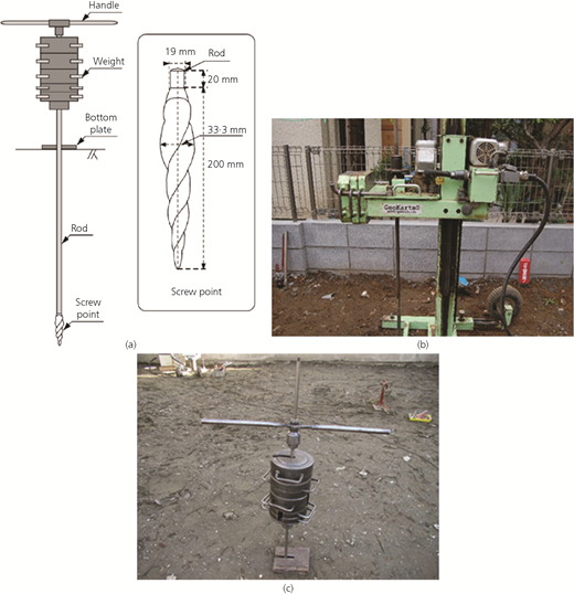
SWS equipment: (a) details of equipment and screw point (after Tsukamoto (2015)); (b) automatic implementation; (c) manual implementation
SWS equipment: (a) details of equipment and screw point (after Tsukamoto (2015)); (b) automatic implementation; (c) manual implementation
While the SWS test is highly portable and simpler than other sounding tests, it has some disadvantages, such as low accuracy in classifying soils and the results are fairly influenced by the rod friction. In cases where the soil contains gravel, the required load to penetrate, the number of half-turns and, consequently, the soil resistance estimated from the SWS tend to be overestimated as the rod friction becomes large.
Suemasa et al. (2005) examined the interaction between the torque and the vertical load during SWS implementation by using miniature SWS model equipment. From the results, they proposed a plasticity-theory-based macroelement model where they indicated that the coefficient of yield locus, c y (which relates the normalised torque and normalised weight applied), and the coefficient of plastic potential, c p (which relates the normalised half-turns and the torque on the rod), vary depending on the soil type – that is, clay, loam, medium sand or dense sand. Hence, they concluded that the soil can be classified based on the data obtained from the SWS if the torque can be measured. This led to further refinements of the SWS in terms of the operating system and resulted in the development of the SDS test.
SDS test
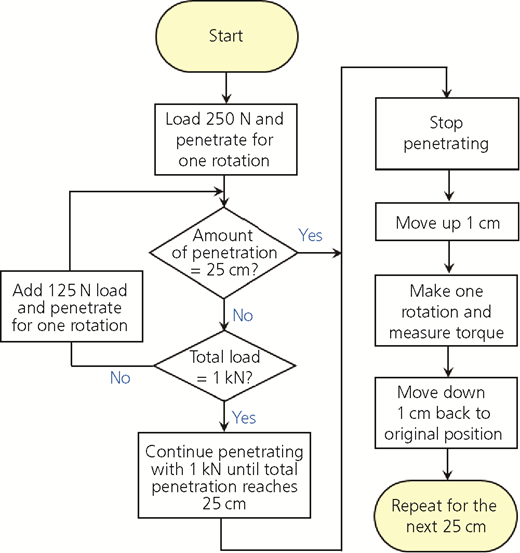
The SDS test is basically an improved system for conducting the SWS test to incorporate a procedure to measure the rod friction and, in the process, minimise the disadvantages of the SWS. In the SDS test, a small portable machine is used to apply the load monotonically in seven steps (0·25, 0·38, 0·50, 0·63, 0·75, 0·88 and 1·0 kN) – that is, the load is increased at every complete rotation of the rod until a 25 cm penetration is reached. During this time, the rod is always rotated at a constant rate (25 revolutions/min). After each 25 cm of penetration, the rod is lifted up by 1 cm and then rotated once to measure the rod friction. Then, it is moved down 1 cm back to its original position, and the process is repeated at every 25 cm of penetration. The parameters measured at every complete rotation of the rod are maximum torque (T max), average torque (T avg), minimum torque on the rod (T min), penetration length (L), penetration velocity (V z) and number of rotations of the rod (N SD). The procedure for performing the SDS test is summarised in Figure 2.
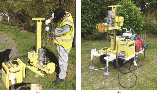
While SWS is usually performed manually (i.e. application of weights and rotation of rods are done with human effort), the need to measure torque and velocity at each step of loading requires the use of a machine. A machine originally used for the SWS test has been revised with some sensors added to incorporate the changes required by the SDS test. Figure 3(a) illustrates the small-scale machine used in conducting SDS; it can be mounted on top of a crawler (see Figure 3(b)) for ease in transport and handling from one site to another. Furthermore, the machine can be disassembled and can easily fit inside a normal van, together with the crawler.
Estimation of friction
Due to the effects of friction on the measured torque and load on the rod during penetration, the measured load and torque required for penetration are greater than the values acting on the screw point. The rod friction that develops as the rod rotates and penetrates into the ground can be divided into a vertical component (W f) and a horizontal component (T f) (Tanaka et al., 2012); the concept is illustrated in Figure 4(a).
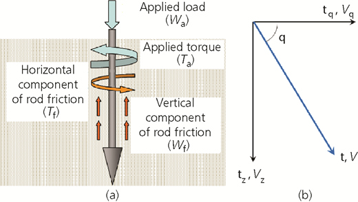
(a) Concept of friction acting on the sounding rod; (b) estimation of rod friction (Tanaka et al., 2012)
(a) Concept of friction acting on the sounding rod; (b) estimation of rod friction (Tanaka et al., 2012)
The load (W a) and torque (T a) applied by the SDS machine are defined as follows
where W and T are the load and torque at the screw point, respectively. The maximum shear stress, τ max, acting on the rod body is computed as follows
where T m is the torque resisting the rod friction measured at the end of a loading set, r is the radius of the rod and L is the amount of penetration. Assuming that the directions of rotation velocity (V θ) and of penetration velocity (V z) are equal to those of the horizontal shear stress (τ θ) and vertical shear stress (τ z) on the rod surface, respectively (see Figure 4(b)), the expressions for the shear stresses are derived as follows
θ can be derived from the ratio between V θ and V z. By substituting Equation 3 into Equations 4 and 5, the vertical and horizontal components of the rod friction are obtained as
Definition of SDS parameters
The authors conducted an extensive research programme through field tests using SDS at various sites in NZ and obtained soil samples at the tested sites for laboratory testing. The objectives of the research were as follows: (a) add data to the existing database of Japanese soils in order to improve the applicability of the SDS to various types of soils; (b) by comparing the SDS results with available data from adjacent CPT/SPT sites and/or borehole logs, provide further data for characterising NZ sites and determine their geotechnical properties; (c) develop empirical correlations to estimate various geotechnical design parameters directly from the SDS data; and (d) explore the possibility of using SDS-derived parameters for soil classification and evaluation of liquefaction potential of sandy deposits.
To date, SDS tests have been performed at 260 sites all over NZ (105 in Auckland, 34 in Wellington and 121 in Christchurch). The majority of the sounding tests were conducted within 2–5 m from CPT/SPT sites or sites with borehole logs, as described in the New Zealand Geotechnical Database (NZGD, 2014). For sites where data were not available, additional CPT tests were conducted. In addition, undisturbed soil samples of cohesive clays and plastic silts were obtained using push tubes at fine-grained sites (generally in Auckland) where SDS tests have been performed, while in SDS sandy sites (generally in Christchurch), disturbed sand samples were obtained by block sampling.
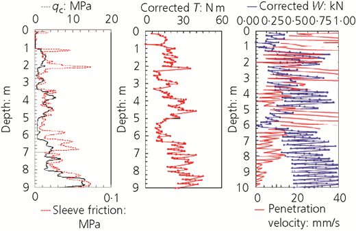
A typical SDS test result is shown in Figure 5. The test was conducted within 2 m of a CPT site and borehole. The SDS plots illustrate the corrected torque and load (for rod friction) and the penetration velocity at every 25 cm, up to a depth of 10 m. Also shown in the figure is the CPT profile (cone resistance, q c, and sleeve friction, f s) available from NZGD. Comparison of the CPT q c and measured torque in SDS indicates a good correlation between the two – that is, the torque required to penetrate the screw point increases with increase in cone penetration resistance. Within a given 25 cm interval, the change in torque as loading steps progress with the application of load appears to increase when the penetration resistance is high. On the other hand, the change in torque in a softer layer is small. Moreover, the penetration velocity significantly decreases when a hard layer is encountered.
More information can be obtained by processing the initial information obtained from SDS, and some of these are illustrated in Figure 6. For example, N SD D is the normalised number of half-turns and is obtained by multiplying the number of half-turns for every 25 cm of penetration (N SD) by the outer diameter of the screw point (D). For the profile shown in Figure 6(a), N SD D is low in the upper 3·5 m and increases below it (depth between 3·5 and 5 m), reflecting the trend in the penetration resistance from the CPT. Another parameter, πT/WD, represents the normalised torque and is defined using the effective torque (T) and the weight (W) as well as the outer diameter of the screw point (D). The variation with depth at this specific site is shown in Figure 6(b). These two indices give an indication of the level of torque required to twist the rod and therefore an index for soil type. In fact, based on the plasticity theory discussed earlier, Suemasa et al. (2005) defined the ratio of these two parameters as the coefficient of plastic potential in terms of SDS tests, c p, as follows
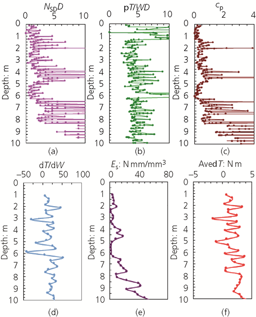
Additional information from SDS data variation with depth of (a) normalised number of half-turns, N SD D; (b) normalised torque, πT/WD; (c) coefficient of plastic potential, c p; (d) change in torque with applied load, dT/dW; (e) specific energy, E s; and (f) average change in torque, AveδT
Additional information from SDS data variation with depth of (a) normalised number of half-turns, N SD D; (b) normalised torque, πT/WD; (c) coefficient of plastic potential, c p; (d) change in torque with applied load, dT/dW; (e) specific energy, E s; and (f) average change in torque, AveδT
Thus, c p is an indication of the difficulty of penetration. From the Japanese database, Tanaka et al. (2012) found that the value of c p varies depending on the type of soil. They noted that the range of c p values for different types of soils is as follows: sand layer: >1·0; silt and clay: 0·3–1·0; and peat and organic soil: <0·3. The distribution of c p in Figure 6(c) appears to indicate generally a silt layer at depths of up to 3·5 m and between 5 and 6·2 m and a sandy soil layer between 3·5 and 5 m and below 7 m; this is consistent with the description indicated in the borehole log. Another parameter, dT/dW, whose depth variation for this site is shown in Figure 6(d), represents the change in torque, T, with the applied weight, W, and is therefore analogous to the slope of the plot of shear stress against confining pressure in conventional laboratory testing.
The combined effect of the applied load and torque during SDS test can be expressed in terms of energy – that is, the incremental work done, δE, by the torque and vertical load for a small rotation can be calculated as (Suemasa et al., 2005)
where δn ht is the number of incremental half-turns and δs t is the incremental settlement caused at a load step. The average specific energy, E s, is defined as the average of the penetration energy E for different loading steps divided by the volume of penetration of the screw point
where L is the amount of penetration, D is the maximum diameter of the screw point and n is the number of steps of loading; this parameter is an indication of the layer stiffness (i.e. the stiffer the soil, the more energy is required to penetrate it). As indicated in Figure 6(e), E s < 10 N mm/mm3 at depths of 0–3 and 5–6 m, consistent with the assumed silt profile, and E s > 10 N mm/mm3 at depths perceived to be sandy.
Finally, the average change in torque, AveδT, shown in Figure 6(f), is defined as
where T is the torque at each step of loading, i, and n is the number of load steps. Generally, AveδT is related to the soil grain size, with high values associated with sandy soil and low values for clayey soils.
Soil classification chart
Considering the SDS tests performed in 38 sites in NZ which were conducted adjacent to sites where borehole logs were available, an attempt was made to determine which SDS parameter(s) would correlate well with the type of soil (determined visually from the borehole logs) found at each depth. Hence, it was possible to come up with a soil classification chart based purely on SDS parameters obtained during the tests. For this purpose, various SDS parameters (expressed in terms of measured torque, load, energy etc.) were investigated to examine which of these best correlate with the appropriate soil types. Based on observation using NZ experience, the parameter cp and AveδT correlate well with the soil type. However, for the purpose of classification, the cp defined in Equation 8 is expressed as the average value of the different loading steps and therefore represents the average at every 25 cm penetration
The soil classification chart obtained based on the NZ soil database is shown in Figure 7.
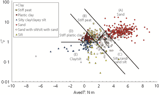
Note that in the figure, the boundary lines are drawn to separate the data visually such that points representing similar soil types are grouped together. Data points in region A are sandy soils, which, because of their frictional nature, are expected to have higher AveδT and values compared with the other soil types. Based on borehole log analysis, sands on the left part of the region are finer than those on the right part. In addition, as is an indication of the difficulty in penetration, the upper part of region A would be denser than those on the lower part. Region B is for stiff peat, which can be found in South Auckland; peat is considered as a c–φ soil, and it is reasonable that it is positioned to the right side of regions D and E, both of which represent cohesive soils. Region C represents sandy silt and silty sands. Soils at the bottom left of the region contain more silt than sand; therefore, this region can be considered as a transition zone from a frictional behaviour to a frictionless (cohesive) one. Soils in region D are highly plastic stiff clays which have AveδT values <1·5 and . Finally, region E, where , belongs to clayey silt, silty clay, silt and clay. Note that the available borehole data for clayey soils in the database were scarce, and more tests are planned to separate clay and silt. However, it is expected that the upper part of this region would represent stiff clay or silt, while the lower part would be for soft clay.
Estimation of parameters from SDS data
SPT N value
SPT is a very popular test around the world, and geotechnical engineers have gained significant experience in designing geotechnical structures using parameters based on SPT correlations. For SDS, more development based on local experience and field observation is required to derive geotechnical parameters from the obtained results. Thus, there is a need for reliable SDS–SPT correlation so that SDS data can be used in conjunction with available SPT design correlations.
For this purpose, SDS tests were performed at sites where SPT had been conducted to compare the SDS output and measured SPT N value. The borehole and SPT data used were obtained from NZGD, and the SDS tests were conducted <2 m away from the preselected sites. It was deemed that only those with clean sand layers would be considered, as the data for other types of soil were very limited. Thus, the soil type was first identified through the borehole log, and then comparisons were made between SDS and SPT on a depth-by-depth basis. Figure 8 illustrates the correlation between SPT N value and specific energy E s from SDS for 18 sandy sites in Christchurch.
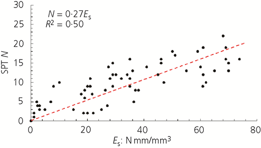
It is observed that while there is scatter in the plots, there is generally a linear relation between the SPT N value and specific energy, E s. As the SPT N value increases, the soil becomes denser and the energy required to penetrate the screw point into the soil increases.
The sources of the scatter in the data points can be traced to the difference in the penetration mechanism and the depth of recording points. Obviously, the penetration in SPT is dynamic, while in SDS, it is static. Also, while SDS recorded the parameters continuously along the depth (and E s was averaged every 25 cm of penetration), the SPT N value was measured every 1 or 1·5 m. In dense to medium dense sands, E s may represent the properties of soil for a layer with thickness of even less than 25 cm (due to difficulty in penetration). At some depths, the average of two successive 25 cm penetration was used in SDS to compare with the SPT N value, and some outliers belonging to transition layers, identified visually by observing the trends of the two tests, were removed from the plot.
As mentioned, this correlation is applicable only to clean sands, and more data are required to extend this relation to other types of soils. In addition, the maximum load and torque that the SDS machine can apply are limited. Thus, in stiff soils, the machine cannot penetrate and the rod just simply rotates without significant penetration and therefore the measured energy does not represent the actual stiffness of soil. Generally, based on experience, SDS can penetrate in soil layers with SPT N value <15.
Fines content
Fines content (F C) in sandy soil plays an important role in the engineering design of geotechnical structures, particularly when the area is prone to earthquakes. The amount of F C significantly influences the liquefaction potential of soil. In engineering practice, it is very common to estimate F C using the CPT data, as this test has become the most common field test for the design of structures. However, experience in Christchurch showed that CPT overestimated the fines content within a soil (Van T Veen, 2015). Hence, an attempt was made to formulate a relationship between the fines content and the SDS parameter(s) as an alternative to the CPT-based estimation.
For this purpose, samples obtained from 18 different sites were considered and sieve analyses were performed on 115 samples. The particle size distribution for each sample was obtained by the method of wet sieving described in NZS 4402.2.8 (Standards NZ, 1986), with F C defined as the percentage by weight passing through a 63 μm sieve. As mentioned earlier, AveδT relates to the grain size of soils; hence, a relationship between F C and AveδT was sought. All the data are compiled and plotted in Figure 9. For AveδT < 0·2 N m, F C can be considered to be 100%; for AveδT > 3·5 N m, the soil can be considered as clean sand (F C < 5%). Between these ranges, the curve shows a good correlation between F C and AveδT.
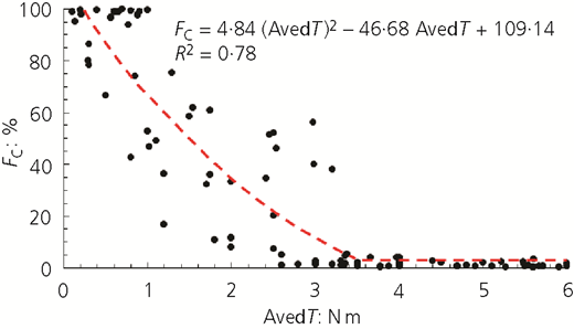
Although the graph shows a good correlation between F C and AveδT, more tests need to be performed, particularly for soils with AveδT < 3·5 N m (including silty sand, sandy silt, clayey sand and sandy clay). It should be mentioned that the plasticity of fines is not taken into consideration in the plot. Further investigation needs to be done to evaluate the applicability of the proposed method when used for other soils. Currently, more tests are planned to refine the developed correlation.
CPT cone tip resistance
In order to develop a correlation between CPT and SDS parameters, SDS tests were conducted <2 m from sites with available CPT data. As in establishing the SPT correlation, the SDS parameters and the CPT cone tip resistance, q c, at similar depths were compared. Among the SDS parameters, the specific energy, E s, best correlated with q c.
By comparing the SDS and CPT data for 60 sites, it was found that the correlation between the outputs from these two tests is highly dependent on the fines content and the stiffness of the soil ( value). The fines content were estimated from the SDS data using Figure 9, with three levels of F C considered: low, medium and high. For soils with high F C, the correlation was different for stiff plastic soils and soft plastic soils. As shown in the soil classification chart in Figure 7, is the threshold separating stiff and soft soils. Thus, for the purpose of developing the correlation, the tested soils were divided into four groups as follows: (a) F C ≤ 5%; (b) 5% < F C < 35%; (c) F C ≥ 35% and ; and (d) F C ≥ 35% and .
Figure 10 illustrates the relationships between E s and q c for different fines contents. Again, it is observed that as the cone penetration resistance increases, the specific energy required to penetrate the screw point in SDS increases. In denser soils with high q c values, the SDS machine cannot penetrate the screw point into the ground and the rod just simply rotates without significant penetration, leading to higher E s. Based on experience, SDS can generally penetrate into soil layers with q c values <15 MPa.
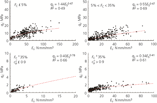
Again, data scatter is seen in the plots, due to the difference in the penetration mechanism (static penetration for CPT and static + rotational penetration in SDS) and the uncertainty associated with depth measurements (CPT was measured every 20 cm, while SDS was recorded every 25 cm). While care was taken when selecting data for analyses, zones in the transition between layers were problematic. Also, many of the CPT and SDS tests were performed with a time gap between them, and it is possible that soil conditions, such as the water table, may have changed during this gap, which could have affected the penetration resistance of soil.
SBT index
While sampling is not possible in conventional implementation of the CPT, the identification of the soil type has been generally accomplished using charts that link cone measurements (cone resistance, q c, and sleeve resistance, f s) to soil type. However, Robertson (1990) stressed that the charts were predictive of SBT since the cone responds to the in situ mechanical behaviour of the soil. Jefferies and Davies (1993) identified that an SBT index, I c, could represent the SBT zones in the chart where I c is essentially the radius of concentric circles that define the boundaries of soil type in the SBT chart. With a way of defining the SBT, CPT has become a powerful tool not only in determining soil stratigraphy and identifying soil type but also in identifying possible microstructure in soils to supplement existing geologic information.
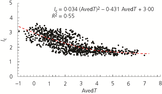
An attempt was made to correlate data from 40 SDS sites in Christchurch and Auckland with the CPT I c values. Subsequent analyses indicate that there is a good correlation between AveδT of SDS and I c of CPT, as shown in Figure 11. It can be seen that this relation is consistent with the recommendations of Robertson (1990, 2010). For example, soils with AveδT > 3·5 would be clean sand to silty sand (I c = 1·31–2·05), and when AveδT < 0·2, it would be silty clay to clay (I c = 2·95–3·6).
Other geotechnical correlations
The research programme also developed correlations between SDS and other geotechnical parameters, such as shear strength parameters (undrained shear strength and angle of international friction) as well as liquefaction potential assessment of sandy soils. However, due to space limitation, the details are not discussed herein.
For example, reconstituted and undisturbed soil samples were obtained from sites in sandy sites in Christchurch and in clayey deposits in Auckland, respectively, and the shear strength parameters were determined using laboratory-based triaxial tests. The undrained shear strength of cohesive soils and the friction angle of sandy soils were then correlated with the SDS results obtained at depths where the soil samples were obtained, and the analyses indicated that the AveδT of SDS best correlated with the shear strength parameters. The correlation equations indicated that as the friction angle or undrained shear strength increased, the average change in torque also increased (Mirjafari et al., 2018).
Moreover, making use of liquefaction observations in Christchurch following the 2010–2011 Canterbury earthquake sequence, a methodology was developed to estimate the liquefaction potential of sites using SDS-derived parameters. By correlating the cyclic resistance ratios of liquefied and unliquefied sites with the specific energy, E s, at appropriate depths, Mirjafari et al. (2016) used logistic regression analyses to develop empirical charts which defined boundary curves delineating different probabilities of liquefaction. They also made use of an artificial neural network (ANN) to predict the liquefaction potential of soil using SDS-derived parameters (Mirjafari et al., 2017). Through their ANN models, they identified that, in addition to E s, other SDS parameters, such as AveδT and penetration velocity V z, and the peak ground acceleration induced by the earthquake, are the important parameters that can be used to predict the liquefaction potential of soil.
Comparison with other in situ tests
Table 1 presents a summary of the comparison between the SDS and other popular in situ tests. As shown in the table, the SDS has many advantages, such as faster implementation (time required for 10 m of penetration is approximately 30 min), simpler system for performing the sounding test, smaller machine size and better cost efficiency compared with other in situ tests. It has great potential as an in situ testing method for geotechnical site characterisation, particularly for residential house construction and roading projects.
Comparison between SDS method and other popular in situ tests
| SDS | SWS (automatic) | SPT | CPT | ||
|---|---|---|---|---|---|
| Basic data | Penetration type | Static and rotational penetration | Static or rotational penetration | Dynamic penetration | Static penetration |
| Penetration ability | N value is around 15 | N value is around 15 | High | Based on load ability | |
| Information obtained | Three components: load, torque and penetration depth | One component: load or half-turns | One component: number of blows (soil type) | Three components: penetration resistance, friction and pore pressure | |
| Estimated information | Soil type, firmness and so on | N value, qu | Firmness | Soil type, strength, liquefaction and consolidation | |
| Workability | Efficiency | Good | Good | Bad | Acceptable |
| Working space | Can be used in narrow places | Can be used in narrow places | Equivalent to two vehicles | A little wide | |
| Installation effort | Easy | Easy | Scaffolding and water supply are required | Anchor casting | |
| Required skill | Not very high | Not high | High | High | |
| Environmental impact | Quiet | Quiet | With noise and vibration | Quiet | |
| Approximate cost for 10 m of penetration:a NZD | 200 | 200 | 2200 | 350 | |
Indicated costs are approximate (mobilisation costs excluded) based on experience in NZ (Ground Investigation Ltd, 2015). 1 NZD = 0·676 USD
Concluding remarks
The SDS method has been recently developed as an improvement of the SWS method. SDS can measure more parameters, including the required torque, load, speed of penetration and rod friction, and can provide a robust way of characterising soil stratigraphy. It is a cost-efficient test which uses a machine-driven and portable device, making it ideal for testing in small-scale and confined areas. Moreover, with a maximum testing depth of 10–15 m (corresponding to roughly SPT N value < 15 and CPT qc < 15 MPa), it is suitable for projects involving residential houses and roading works.
For the purpose of improving the current understanding of SDS tests in terms of characterising soil and site profiles, a total of 260 tests were conducted in NZ adjacent to available CPT/SPT and borehole locations. From the developed SDS soil database, a soil classification chart based purely on SDS parameters was established where a variety of soil types were included, such as sand and silty sand in Christchurch and Wellington, and peat or clayey soil in Auckland.
A linear correlation was observed between the SPT N value and specific energy Es of SDS. Similarly, by performing sieve analysis on the samples obtained from SDS sites, a correlation was found between AveδT of SDS and FC. Moreover, correlations were also developed between SDS parameter(s) and CPT cone resistance and SBT index.
Finally, a comparison was made between popular in situ tests in terms of their basic data and workability. Compared with other tests, SDS is simpler and it does not need a large space to conduct the test; by measuring a variety of parameters continuously (including torque, load and speed of penetration), it can give a clear image of the soil profile.
Acknowledgements
The authors would like to acknowledge Nitto Seiko Company for providing the SDS machine and the Japan Home Shield Corporation for providing assistance for this research. They would also like to acknowledge the New Zealand Geotechnical Database for providing the borehole data and SPT/CPT records in the target sites and the city councils for providing access to the test sites. In addition, the assistance of several undergraduate students of the University of Auckland in performing the laboratory tests is also acknowledged.

