
The difficulties of engineers and managers agreeing on how to invest in infrastructure maintenance stem from a basic inability to communicate with each other. This leads to the suboptimal management of infrastructure. Luckily, this situation can be remedied by engineers learning how to communicate their concerns in a way that managers can understand, so that they can clearly see whether a proposed action needs to be taken or can be deferred. This paper shows, with the help of a realistic example, in terms of infrastructure, methodology and techniques, how this can be done. The proposed approach, although upon reading is perhaps intuitive, is starkly absent in the literature in the field of infrastructure asset management. In the proposed approach, it is demonstrated how to improve the traditional approaches used by engineers to communicate to managers through (a) the quantification of the level of service as seen by mangers, (b) the modelling of how infrastructure might not provide the required level of service and (c) the way of showing how intervention programmes can affect the provision of service, both now and in the future.
Introduction
Management of infrastructure often involves engineers and managers. Engineers, who are assumed in this paper to be those people responsible for deciding exactly what is to be done with pieces of infrastructure, are people with a technical background who are concerned about the details of how infrastructure functions, how it might fail and the processes that can cause this. Managers, who are assumed in this paper to be those people responsible for deciding how to allocate money for entire portfolios of infrastructure objects including across districts and regions, are people with a business background who are concerned with ensuring that infrastructure can meet the demands of it. Engineers and managers are working on the same team. Due to their different backgrounds, however, they sometimes have difficulty communicating with each other. This needs to be changed. The approach proposed in this paper, regardless of the infrastructure analysed or specific methodology or techniques used, bridges this gap. The proposed approach, although upon reading is perhaps intuitive, is one that has not yet been proposed in the field of infrastructure asset management.
In order to understand how this can be done, one needs to have a common understanding of infrastructure and infrastructure management. Infrastructure, at least in this paper, is considered to be the fixed physical objects that are needed to provide a service – for example, to allow people to travel between two cities within an hour. Infrastructure management is the process used to ensure that the infrastructure provides the service expected from it – for example, planning and executing interventions to prevent bridges from collapsing on the road between the two cities. The key for engineers and managers to understand each other is to focus on the service provided by the infrastructure. If it is accepted that infrastructure exists only to provide service, it becomes impossible to make reasonable decisions pertaining to infrastructure without explicitly considering it. Indeed, this is why there is room for improvement in many of the discussions between engineers and managers, as engineers do not frame their arguments, normally, in the language of why infrastructure is there. Instead, they focus on parts of the big picture, talking often about reliability, availability and safety. These parts are by all means important, but they are only proxies for what really matters – that is, service.
In order for engineers and managers to communicate and to understand the contents of this paper, it is not only the definitions of these words that need to be clear, but also how they relate to service. The definitions used in this paper are given in Table 1. These definitions were chosen by the authors to facilitate the writing of the paper. Of course, other definitions for these words are possible, but these ones nicely and clearly link them to the point of having infrastructure – that is, to provide service. Other definitions would not change the approach proposed in the paper or the ability to demonstrate its effectiveness. If other definitions or other proxies – for example, affordability – are used, they should also be tied to the service provided. Many discussions between engineers and managers end in frustration in the absence of clarity in these matters.
Proxies
| Proxy | Definition |
|---|---|
| Availability | The amount of time that the travel time costs are below the maximum allowed travel time costs divided by the total time |
| Reliability | The probability that the costs will be lower than the maximum agreed on costs |
| Safety | The probability of occurrence of accidents in which there are injuries or fatalities multiplied by the unit value of the injuries and fatalities |
| State | The physical condition of the infrastructure |
Literature review
There has been in the past an extensive and growing amount of literature on decision making with respect to infrastructure. This can be grouped as literature focused on (a) technical aspects, such as reliability, availability and safety; (b) multicriteria decision analysis, which is focused on weighting more than one criteria in often subjective ways; and (c) cost–benefit analysis. The literature in all three categories contains text stemming from research and from practice in the form of guidelines or supporting software. Some of the most representative literature in each category is presented and discussed in the next three sections.
Technical aspects
There is in literature an abundance of examples where justification for infrastructure decisions are given based primarily on technical aspects, which are essential used as proxies for providing service. In every case, the quantification of how service might be affected would enable better decisions to be made. A few of the examples found in literature are given in Table 2, which includes, per example, the technical criteria used, the decision made and an example improvement. Table 2 is to be read as follows: it is reported in Calle-Cordon et al. (2017) that the technical criteria reliability, availability, maintainability and safety can be used to determine the interventions to be executed on switches and crossings. An improvement in the determination of the interventions to be executed can be obtained by additionally quantifying the costs of lost service in any situations when they might occur. For each reference, only one example is given. By following the proposed approach, such improvements would be ensured.
Examples of technical aspects used as proxies in infrastructure decision making
| Reference | Technical criteria | Decision made | An improvement would be to quantify additionally … |
|---|---|---|---|
| Calle-Cordon et al. (2017) | Reliability, availability, maintainability and safety | Interventions to be executed on switches and crossings | Costs to users of lost service |
| Patra (2009) | Reliability, availability, maintainability and safety | Interventions to be executed on railway infrastructure | Costs to users of lost service |
| Zio et al. (2007) | Reliability of objects, delays due to speed restrictions caused by deteriorated conditions and interventions | Interventions to be executed on tracks | Risks related to delays |
| Jaedicke et al. (2013) | Probability of being hit by a landslide | Rank of objects for intervention | Costs of being hit |
| Liu et al. (2014) | Probability of collision between cars and trains at level crossings | Rank of level crossings for intervention | Costs of travel delays in case of collisions at level crossings |
| Jafarian and Rezvani (2012) | Probability of derailment, the condition of objects | Rank of objects for intervention | Costs of possible accidents and traffic interruptions |
| Peterson and Church (2008) | Consequences on network operation in terms of traffic flow | Rank of bridges and tunnels for intervention | Costs of losing network operation |
| Kurauchi et al. (2009) | Consequences on network operation in terms of traffic flow | Rank of links for intervention | Risks related to network operation |
| Fecarotti et al. (2015) | Probability and duration of loss of network operation | Rank of railway tracks, switches and stations for intervention | Risks related to network operation |
| Chang and Nojima (2001) | Consequences on network operation in terms of traffic flow | Estimate infrastructure disruption and restoration costs after earthquakes | Risks related to network operation after earthquakes |
| Sun and Gu (2011) | Roughness, deflection, surface deterioration, rutting, skid resistance | Road interventions to execute | Costs of reductions in service due to increased roughness |
Multicriteria decision analysis
There is in literature an abundance of examples where justifications for infrastructure decisions are given based on the results of multicriteria decision analysis. Some of these works assign values to multiple technical aspects, some combine technical aspects and estimations of level of service and some combine estimations of the level of service without reverting to direct valuation of the levels of service – that is, costs. In every case, a direct valuation of how the infrastructure might not provide service would enable better decisions to be made. A few examples of each of these are given in Tables 3 and 4, which include a summary of the criteria used, the decision made and an example improvement. Tables 3 and 4 are to be read as follows: it is reported by Carretero et al. (2003) that the probability of failure multiplied by the costs of restoring the infrastructure can be used to determine which interventions to be executed on tracks. An improvement can be obtained by additionally quantifying the costs of injuries, fatalities, damaged equipment and downtime due to failures when they might occur. For each reference, only one example is given. By following the proposed approach, such improvements would be ensured.
Examples of multicriteria decision analysis in infrastructure decision making (1/2)
| Reference | Technical criteria | Decision made | An improvement would be to quantify additionally … |
|---|---|---|---|
| Carretero et al. (2003) | Probability of failure multiplied by the costs of restoring the infrastructure | The interventions to be executed on tracks | The costs of injuries, fatalities, damaged equipment and downtime due to failures |
| Stein et al. (1999) | The probability of scour at bridge foundations, cost of maintenance, cost of passenger delay | The rank of bridges for intervention | The costs of injuries and fatalities due to bridge failures |
| Cheng and Tsao (2010) | Reliability, travel time, passenger safety, quality of service, intervention costs | The interventions to be executed on rolling stocks | The costs of injuries and fatalities due to bridge failures |
| Celebi et al. (2008) | Quality of service, travel time, spare part costs, storage costs | The interventions to be executed on tracks | The costs of lost quality of service |
| Ebrahimnejad et al. (2012) | Staff required, project duration, fit with company fit, with objectives and policy, fit with budget, risk/return ratio, fit with regulations, fit with standards, fit with terms of contract, ability of management to execute, ability to avoid conflicts, contribution to environmental protection, contribution to health and safety, knowledge regarding the technology to be used | The track to be installed | The costs of injuries and fatalities due to heavy rain |
Examples of multicriteria decision analysis in infrastructure decision making (2/2)
| Reference | Technical criteria | Decision made | An improvement would be to quantify additionally … |
|---|---|---|---|
| Caterino et al. (2006) | Service interruption during interventions, cost of construction; cost of interventions | The seismic retrofitting interventions to be executed on a reinforced-concrete structure | The costs of service interruption |
| Dawotola et al. (2009) | Externalities, corrosion, operational errors, structural defects, cost of interventions | The design, construction, inspection and maintenance strategy for petroleum pipelines | The costs of lost service due to deterioration |
| Frangopol and Liu (2007), Liu and Frangopol (2004) | Costs of intervention, safety, condition, environmental impact | The bridge intervention strategy | Failure costs |
| Guhnemann et al. (2012) | Costs of intervention, safety, environmental impact | The road intervention strategy | Failure costs |
| Guhnemann et al. (2012) | Importance of the project and the sector, cost of intervention and suitability of finance, execution and operation, probability of failure and consequences of failure of the infrastructure | The urban infrastructure projects to finance | The costs of delays and accidents |
Cost–benefit analysis
There is in literature an abundance of examples where justification for infrastructure decisions are given based on the results of cost–benefit analysis. These works often attempt to quantify all effects on service by assigning to them either costs or utility. They often, however, do not cover all important aspects of service. A few examples of each of these are given in Table 5, which includes a summary of the costs and benefits used, the decision made and an example of service not covered. Table 5 can be read as follows: it is reported by Peng (2011) that the decision of how to group interventions on tracks can be made by taking into consideration the costs of intervention and the costs of network operation. An improvement, however, would be to take additionally into consideration accident costs. For each reference, only one example is given. By following the proposed approach, such improvements would be ensured.
Examples of cost–benefit analysis in infrastructure decision making
| Reference | Costs and benefits | Decision made | A further improvement would be to quantify … |
|---|---|---|---|
| Peng (2011), Peng and Ouyang (2014) | Costs of intervention, costs of network operation | How to group interventions on tracks | Accident costs |
| Zhao et al. (2006) | Costs of intervention | Ballast tamping intervention strategy | Accident and travel time costs |
| Budai-Balke (2009) | Costs of intervention | Track intervention strategy | Accident cost |
| Thoft-Christensen (2009) | Costs of intervention | Bridge intervention strategy | Accident cost |
| Zhang et al. (2013) | Costs of intervention, safety, travel disruption | Track intervention strategy | Travel time costs |
| Lyngby et al. (2008) | Cost of intervention, cost of failure (i.e. cost of unavailability of service due to failure) | Interventions to be executed on tracks | Risks related to accidents, costs for traffic interruption due to preventive interventions |
Summary
The literature review shows that many people are concerned with making the right decisions with respect to maintaining infrastructure. It also clear, though, that everyone is looking at only part of the problem, either by not explicitly relating things to the service provided or by not capturing all of the relevant service provided. This means that when they present their ideas to a manager, the manager, presented with an incomplete picture, loses confidence in what it presented and knows it does not fully represent what they care about. This forces or enables them to revert comfortably to his own preformed opinions. This leaves frustrated engineers, on the less serious side of things, but also to managers making suboptimal decisions with respect to their infrastructure, on the more serious side of things. The latter can lead to unnecessary wasting of money now or in the future, unnecessary increases in user disturbances now or in the future or, even worse, unnecessary increases in the number of accidents that may happen.
Steps
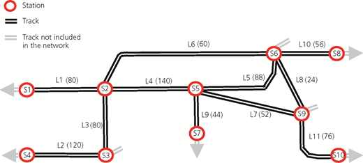
In order for engineers to be able to communicate their concerns – for example, with respect to risk, reliability, availability and safety – to managers in a way that they can understand, engineers need to realise what is important to managers. Managers are not interested in the technical aspects. They operate at the system level and are concerned with how their infrastructure is going to function as a whole and how the infrastructure is going to provide service. They are interested only in taking action to fix a technical issue if they feel that how their infrastructure functions as a whole is in jeopardy and the costs of doing so are justified. This means that the engineers have to be able to show that the state of the infrastructure leads to negative impacts on, or costs to, the stakeholders. As managers are concerned with not only right now, but also the future, engineers must be aware that they have to be sure to convey to managers that they know, and have modelled well, not only how the entire system functions now but also how it functions in the future. As one cannot, of course, model everything, the engineer, when communicating with managers, needs to be sure that they cover all aspects that are of concern to the managers and models the differences of what will happen when the engineer’s advice is followed and when not. Additionally, engineers must ensure that when it comes to displaying the results of their simulations that they focus on the things that matter to managers at the right level and not on the things that are important to the engineer. Of course, the models that are used for communication do not replace the ones required by the engineers to propose very specific answers to specific problems, but are rather built on top of, or in conjunction to, these models. The four basic steps to ensure that engineers can speak to managers are described in the next four subsections, using a fictive but realistic railway network (Figure 1), where it is hoped to determine how much money is to be spent on maintenance. The network consists of 86 bridges with a total deck surface area of 20 076 m2, 73 track sections measuring a total of 211 242 m length, 66 earthworks measuring a total of 360 261 m3 and 130 switches. The numbers of trains per day on each of the 11 links are given in Table 6, and each carry on average 100 passengers.
Links in the network with the daily train traffic per link
| Link | From–to | Trains per day | Link | From–to | Trains per day | Link | From–to | Trains per day |
|---|---|---|---|---|---|---|---|---|
| L1 | S1–S2 | 80 | L5 | S5–S6 | 88 | L9 | S5–S7 | 44 |
| L2 | S4–S3 | 120 | L6 | S2–S6 | 60 | L10 | S6–S8 | 56 |
| L3 | S3–S2 | 80 | L7 | S5–S9 | 52 | L11 | S9–S10 | 76 |
| L4 | S2–S5 | 140 | L8 | S6–S9 | 24 | N/A | N/A | N/A |
In order to conduct the example, a relatively common methodology and relatively common techniques are used. As the goal of the paper is to explain an approach that can be used by engineers to communicate in terms of service to the manager, the details of the used methodology and tools are intentionally omitted. This omission helps to keep focus on the goal of the paper and avoids giving the impression that the authors are suggesting the use of a specific methodology or specific techniques.
Provide a complete description of the infrastructure (step 1)
The first step is to provide a complete description of the infrastructure to be included in the analysis – complete, but not necessarily deep, or only as deep as necessary. For example, an infrastructure manager needs to know that all objects that are required to provide the required service are included in the evaluation – for example, all earthworks, all tracks, all bridges and all switches – but it is not necessary for them to know that each beam in steel bridge number 10 is modelled exactly. It is also not of much use to them if someone is conducting an evaluation with just bridges, even if modelled in lots of detail. The most they will get out of such an analysis is a prioritisation of which bridges should have an intervention in the next planning period and how much they would cost. They will, however, most likely be left with no idea of how to compare the need for expenditure on the most important bridge with the interventions required on the track sections, the earthworks or switches. The usefulness of the evaluation for the manager decreases significantly without covering all of the objects and all of the objects in the same way. All of the objects in the example network in this paper, and their four possible states, which cover all possible states in which they can be, are shown in Tables 7 and 8 per link, classified by object type. The object types consist of three bridge types (metal, concrete and masonry), one track type (track), two earthwork types (embankment and cutting) and one switch type (turnout). The tables are to be read as follows: of all of the metal bridges, there are none to be found on link 1 in any state, one in state 1 which measures 32 m2 and one in state 2 which measures 19 m2 on link 2, two in state 2 which together measure 127 m2 on link 3, one in state 1 which measures 104 m2 on link 4, five in state 1 which measure 311 m2, four in state 2 which measure 561 m2, five in state 3 which measure 443 and one in state 4 which measures 70 m2 on link 5 and one in state 1 which measures 124 m2 on link 6. The bridges are measured in square metres of deck surface area.
Number and extent of objects in each state for links 1–6
| Object type | Unit | State | L1 | L2 | L3 | L4 | L5 | L6 | |||||||
|---|---|---|---|---|---|---|---|---|---|---|---|---|---|---|---|
| Number | Extent | Number | Extent | Number | Extent | Number | Extent | Number | Extent | Number | Extent | ||||
| Bridge | Metal | m2 | 1 | 0 | 0 | 1 | 32 | 0 | 0 | 1 | 104 | 5 | 311 | 1 | 124 |
| 2 | 0 | 0 | 1 | 19 | 2 | 127 | 0 | 0 | 4 | 561 | 0 | 0 | |||
| 3 | 0 | 0 | 0 | 0 | 0 | 0 | 0 | 0 | 5 | 443 | 0 | 0 | |||
| 4 | 0 | 0 | 0 | 0 | 0 | 0 | 0 | 0 | 1 | 70 | 0 | 0 | |||
| Concrete | m2 | 1 | 0 | 0 | 0 | 0 | 0 | 0 | 0 | 0 | 0 | 0 | 0 | 0 | |
| 2 | 0 | 0 | 0 | 0 | 0 | 0 | 0 | 0 | 1 | 17 | 0 | 0 | |||
| 3 | 0 | 0 | 0 | 0 | 0 | 0 | 0 | 0 | 0 | 0 | 0 | 0 | |||
| 4 | 0 | 0 | 0 | 0 | 0 | 0 | 0 | 0 | 0 | 0 | 0 | 0 | |||
| Masonry | m2 | 1 | 0 | 0 | 0 | 0 | 0 | 0 | 0 | 0 | 4 | 991 | 0 | 0 | |
| 2 | 0 | 0 | 1 | 60 | 0 | 0 | 0 | 0 | 4 | 2987 | 1 | 211 | |||
| 3 | 0 | 0 | 0 | 0 | 0 | 0 | 0 | 0 | 2 | 363 | 0 | 0 | |||
| 4 | 0 | 0 | 0 | 0 | 0 | 0 | 0 | 0 | 0 | 0 | 0 | 0 | |||
| Track | m | 1 | 0 | 0 | 5 | 4716 | 7 | 13 541 | 0 | 0 | 1 | 360 | 0 | 0 | |
| 2 | 0 | 0 | 4 | 4748 | 6 | 76 876 | 3 | 6363 | 0 | 0 | 2 | 15 249 | |||
| 3 | 2 | 31 495 | 2 | 622 | 4 | 405 | 1 | 520 | 3 | 583 | 0 | 0 | |||
| 4 | 0 | 0 | 0 | 0 | 0 | 0 | 1 | 4068 | 1 | 4291 | 0 | 0 | |||
| Earthwork | Embankment | m3 | 1 | 1 | 905 | 1 | 2107 | 0 | 0 | 0 | 0 | 0 | 0 | 0 | 0 |
| 2 | 0 | 0 | 0 | 0 | 0 | 0 | 0 | 0 | 0 | 0 | 0 | 0 | |||
| 3 | 0 | 0 | 2 | 7736 | 0 | 0 | 0 | 0 | 0 | 0 | 0 | 0 | |||
| 4 | 0 | 0 | 0 | 0 | 0 | 0 | 0 | 0 | 0 | 0 | 0 | 0 | |||
| Cutting | m3 | 1 | 0 | 0 | 0 | 0 | 1 | 3488 | 4 | 28 695 | 2 | 12 016 | 1 | 2831 | |
| 2 | 0 | 0 | 0 | 0 | 1 | 2598 | 3 | 6702 | 2 | 2606 | 4 | 1952 | |||
| 3 | 0 | 0 | 0 | 0 | 1 | 329 | 2 | 7288 | 1 | 5765 | 3 | 15 051 | |||
| 4 | 1 | 616 | 0 | 0 | 1 | 4981 | 0 | 0 | 0 | 0 | 1 | 3105 | |||
| Switch | Turnout | Number | 1 | 0 | 5 | 9 | 5 | 3 | 1 | ||||||
| 2 | 0 | 3 | 10 | 4 | 3 | 3 | |||||||||
| 3 | 0 | 6 | 12 | 0 | 2 | 1 | |||||||||
| 4 | 0 | 1 | 2 | 0 | 0 | 0 | |||||||||
Number and extent of objects in each state for links 7–11
| Object type | Unit | State | L7 | L8 | L9 | L10 | L11 | Total | |||||||
|---|---|---|---|---|---|---|---|---|---|---|---|---|---|---|---|
| Number | Extent | Number | Extent | Number | Extent | Number | Extent | Number | Extent | Number | Extent | ||||
| Bridge | Metal | m2 | 1 | 0 | 0 | 1 | 208 | 4 | 785 | 0 | 0 | 0 | 0 | 13 | 1564 |
| 2 | 2 | 495 | 0 | 0 | 6 | 1771 | 0 | 0 | 0 | 0 | 15 | 2973 | |||
| 3 | 0 | 0 | 1 | 104 | 1 | 154 | 3 | 373 | 0 | 0 | 10 | 1074 | |||
| 4 | 0 | 0 | 0 | 0 | 0 | 0 | 1 | 30 | 0 | 0 | 2 | 100 | |||
| Concrete | m2 | 1 | 0 | 0 | 3 | 774 | 0 | 0 | 0 | 0 | 2 | 208 | 5 | 982 | |
| 2 | 0 | 0 | 3 | 357 | 0 | 0 | 0 | 0 | 1 | 104 | 5 | 478 | |||
| 3 | 0 | 0 | 0 | 0 | 0 | 0 | 0 | 0 | 0 | 0 | 0 | 0 | |||
| 4 | 0 | 0 | 0 | 0 | 0 | 0 | 0 | 0 | 0 | 0 | 0 | 0 | |||
| Masonry | m2 | 1 | 0 | 0 | 4 | 1266 | 2 | 1147 | 2 | 1251 | 2 | 603 | 14 | 5258 | |
| 2 | 0 | 0 | 2 | 119 | 1 | 208 | 1 | 1042 | 2 | 167 | 12 | 4794 | |||
| 3 | 0 | 0 | 2 | 566 | 1 | 208 | 2 | 938 | 2 | 629 | 9 | 2704 | |||
| 4 | 0 | 0 | 0 | 0 | 0 | 0 | 0 | 0 | 1 | 149 | 1 | 149 | |||
| Track | m | 1 | 2 | 174 | 4 | 447 | 1 | 65 | 2 | 19 464 | 1 | 0 | 23 | 38 768 | |
| 2 | 2 | 1447 | 7 | 1253 | 3 | 2544 | 2 | 66 | 0 | 19 330 | 29 | 127 877 | |||
| 3 | 1 | 69 | 3 | 1217 | 0 | 0 | 0 | 0 | 1 | 521 | 17 | 35 431 | |||
| 4 | 0 | 0 | 2 | 807 | 0 | 0 | 0 | 0 | 0 | 0 | 4 | 9166 | |||
| Earthwork | Embankment | m3 | 1 | 0 | 0 | 1 | 2414 | 3 | 6899 | 0 | 0 | 0 | 0 | 6 | 12 325 |
| 2 | 0 | 0 | 5 | 22 246 | 2 | 978 | 4 | 11 072 | 0 | 0 | 11 | 34 297 | |||
| 3 | 0 | 0 | 2 | 13 126 | 2 | 15 783 | 2 | 4754 | 0 | 0 | 8 | 41 399 | |||
| 4 | 0 | 0 | 0 | 0 | 0 | 0 | 0 | 0 | 0 | 0 | 0 | 0 | |||
| Cutting | m3 | 1 | 2 | 56 498 | 0 | 0 | 0 | 0 | 1 | 12 911 | 3 | 62 590 | 14 | 179 028 | |
| 2 | 2 | 18 319 | 1 | 12 616 | 0 | 0 | 0 | 0 | 0 | 0 | 13 | 44 793 | |||
| 3 | 0 | 0 | 0 | 0 | 0 | 0 | 0 | 0 | 3 | 7379 | 10 | 35 812 | |||
| 4 | 0 | 0 | 0 | 0 | 0 | 0 | 0 | 0 | 1 | 3906 | 4 | 12 607 | |||
| Switch | Turnout | Number | 1 | 3 | 8 | 0 | 2 | 4 | 40 | ||||||
| 2 | 7 | 12 | 2 | 1 | 1 | 46 | |||||||||
| 3 | 4 | 10 | 1 | 1 | 2 | 39 | |||||||||
| 4 | 0 | 2 | 0 | 0 | 0 | 5 | |||||||||
The level at which the object types are defined is selected to provide a balance between understanding of the objects in the network and providing an overview of all of the objects in the network. Not all engineers would be happy with this classification. Engineers have a tendency to want more details than necessary and are often too willing to sacrifice the overview, or, in other words, engineers are often not willing to work at a high-level abstraction. As managers have to work at a high level of abstraction, as there is only so much time to obtain an overview, engineers have to as well if they want to provide an overview in a way that a manager will understand. For example, if one treated the objects in the network individually, instead of grouping them together and looking at them as seven types of objects (Tables 7 and 8), a manager would need to look at all 355 individual objects, which is a drastic increase in analysis effort and the manager risks getting lost in the details. The right level of abstraction depends on the time of both the engineer and the manager.
Define clearly who and what is important (step 2)
The next thing that needs to be determined is who and what is important. Engineers often make the mistake of thinking that managers are interested in the technical details. Perhaps they are, but they do not give it first priority. Primarily, managers care about the service that they are providing and how non-functioning infrastructure may affect this service. In order to identify this, one needs to know the stakeholders and how they will be affected if the infrastructure does not work as intended. The clearest way to do this is to express how each stakeholder is affected per unit that can be measured over time and to which people can attribute monetary values. In the example presented in this paper, it is assumed that there are only two stakeholders who can be affected in three different ways: the owner, who is affected by having to pay for interventions and the users who are affected by losing travel time and being involved in accidents. Although many more stakeholders are possible, as are many more ways of how they are affected, these are sufficient to make the point – that is, that engineers have to take into consideration everything that is important to the manager. For example, in the situation presented in the example, if an engineer is telling a manager that an intervention on a bridge is required to save lives, the manager is wondering if the engineer is giving adequate consideration to the intervention costs and the additional travel time costs that will be incurred from executing the intervention, in addition to loss of life, that will occur if a failure leads to an accident. Unless the engineer has in mind all of the same stakeholders and how they are affected as the manager, their argument will not carry much weight.
To facilitate the explanation of how stakeholders are affected, impacts should be broken down into units that can be measured over time and to which monetary values can be associated. Breaking down the impacts per unit time is necessary to ensure that there is a clean separation between (a) the modelling of the infrastructure and the system in which it is embedded and (b) enabling decision makers to assign values to things that are directly comparable in ways that can be easily argued over and discussed, without additional modelling. One can, for example, easily assign a monetary value to 1 h of additional travel time and reasonably discuss how this value compares to the cost of fixing a track section. One cannot, however, easily assign a monetary unit to an increase in system reliability and reasonably discuss how this value compares to the costs of fixing a track section. This is because reliability is a system characteristic that gives a manager an idea of which possible future scenarios are likely – that is, failure or no failure – but does not say how stakeholders are affected. It is without doubt an interesting value, but not one that is directly useable in making decisions of where interventions on a network are to be executed.
The ways that the stakeholders are considered to be affected in the example are shown in Table 9 – that is, these are things on which a value will be put on. It is to be read as follows: the owner is a stakeholder to whom intervention costs are attributed – that is, the owner has to pay for interventions. The amount that the owner pays for the intervention is the cost of the material, machinery and labour required to execute interventions – that is, the economic impact. This cost is estimated by amount they pay for manual labour, machinery and materials listed on the final bills of executed interventions. These costs are estimated by multiplying the number and extent of interventions to be executed and the unit costs of the intervention, which vary as a function of the intervention executed. Monetary values are used instead of others – for example, utility – because they are the intuitive unit used to put values on things. By leaving out a cost to the user of not making a trip, it is being assumed that the number of people who no longer make trips multiplied by the value of these lost trips is negligible. Even if trains do not run, it is assumed that replacement buses will be used. Only passenger travel time is considered. It is assumed that all property damage costs are attributed to the user, including the train operators. This does not mean that the owner will not pay for them in the end – for example, through insurance. A complete list for railways, including the ability to transport freight, can be found in the publication by Papathanasiou et al. (2016) and that for roads can be found in the paper of Adey et al. (2012), and how they change over time in the publications of Adey et al. (2012) and Adey (2017). For clarity, it is pointed out that it is important to define the stakeholders and how they are affected per system being analysed, taking into consideration the decision to be made and the stakeholders involved. The example given in this paper is only for illustrative purposes. An example of something not included is the value that the general population, as stakeholders, would put on negatively affecting the environment – for example, emitting more than the expected carbon dioxide (CO2). A more detailed discussion of such issues can be found in the publication by Adey et al. (2012).
Stakeholders and how they are affected
| Stakeholder | Costs | |||||
|---|---|---|---|---|---|---|
| Label | Description | Estimated by … | Indicator | Unit | Unit cost: €/unit | |
| Owner | Interventions | The economic impact of material, machinery and labour to execute interventions | The cost of manual labour, machinery and materials listed on the final bills of executed interventions – that is, cost of intervention | The type and extent of interventions executed | Extent of interventions | Tables 18 and 19 |
| Users | Travel time | The economic impact of a passenger losing time | The additional travel time required when an intervention is being executed and no intervention being executed multiplied by the unit cost | The additional travel time required when trains cannot travel at the reference speed | Minutes of additional travel time | 0·5 |
| Accidents | The economic impact of having property damaged in an accident | The cost of repairing the damaged property | The extent of damaged property | Number of accidents | 100 000 | |
| The societal impact of being injured in an accident | The number of injuries multiplied by the average amount that society is willing to pay to avoid being injured | The number of injuries | Number of people | 50 000 | ||
| The societal impact of being killed in an accident | The number of fatalities multiplied by the average amount that society is willing to pay to avoid being killed | The number of fatalities | Number of people | 1 000 000 | ||
Explain clearly how the system will be modelled (step 3)
Once it is established how the impacts are connected with the object states, for those that can be directly connected to object states, how the system is to be modelled needs to be explained clearly. This includes (a) how objects change over time, (b) how the level of service required from the objects changes over time, (c) how future scenarios for the infrastructure are determined and (d) how stakeholder costs are estimated. These points are explained in succession in the following sections.
How objects change over time
The state of an object deteriorates and is improved through the execution of interventions over time. It needs to be clear how the changes of state over time are modelled. In the example presented in this paper, this is done with transition probabilities – that is, each object has a probability of transitioning from one state to another in 1-year periods, which depend on whether the object is deteriorating (Table 10) or being improved through the execution of an intervention (Tables 11 and 12). Each object is modelled independently – that is, the possibility of correlated failures is neglected. Even though it is clear that this is an approximation (Adey et al., 2004), this assumption greatly simplifies the overview for infrastructure managers. More information on how the values shown in Table 17 are combined to show the evolution of state over time can be found in Adey and Hajdin (2011).
Probabilities of moving from one state to another in time intervals when no preventive interventions are executed
| Object type | State at t | State at t + 1 | Object type | State at t | State at t + 1 | ||||||||
|---|---|---|---|---|---|---|---|---|---|---|---|---|---|
| 1 | 2 | 3 | 4 | 1 | 2 | 3 | 4 | ||||||
| Bridge | Metal | 1a | 0·95 | 0·05 | 0·00 | 0·00 | Earthwork | Embankment | 1 | 0·85 | 0·15 | 0·00 | 0·00 |
| 2 | 0·00 | 0·98 | 0·02 | 0·00 | 2 | 0·00 | 0·97 | 0·03 | 0·00 | ||||
| 3 | 0·00 | 0·00 | 0·97 | 0·03 | 3 | 0·00 | 0·00 | 0·96 | 0·04 | ||||
| 4 | 0·00 | 0·00 | 0·00 | 1·00 | 4 | 0·00 | 0·00 | 0·00 | 1·00 | ||||
| Concrete | 1 | 0·99 | 0·01 | 0·00 | 0·00 | Cutting | 1 | 0·87 | 0·13 | 0·00 | 0·00 | ||
| 2 | 0·00 | 0·97 | 0·03 | 0·00 | 2 | 0·00 | 0·98 | 0·02 | 0·00 | ||||
| 3 | 0·00 | 0·00 | 0·90 | 0·10 | 3 | 0·00 | 0·00 | 0·97 | 0·03 | ||||
| 4 | 0·00 | 0·00 | 0·00 | 1·00 | 4 | 0·00 | 0·00 | 0·00 | 1·00 | ||||
| Masonry | 1 | 0·94 | 0·06 | 0·00 | 0·00 | Switch | Turnout | 1 | 0·50 | 0·50 | 0·00 | 0·00 | |
| 2 | 0·00 | 0·91 | 0·09 | 0·00 | 2 | 0·00 | 0·84 | 0·16 | 0·00 | ||||
| 3 | 0·00 | 0·00 | 0·95 | 0·05 | 3 | 0·00 | 0·00 | 0·70 | 0·30 | ||||
| 4 | 0·00 | 0·00 | 0·00 | 1·00 | 4 | 0·00 | 0·00 | 0·00 | 1·00 | ||||
| Tracks | 1 | 0·70 | 0·30 | 0·00 | 0·00 | ||||||||
| 2 | 0·00 | 0·90 | 0·10 | 0·00 | |||||||||
| 3 | 0·00 | 0·00 | 0·84 | 0·16 | |||||||||
| 4 | 0·00 | 0·00 | 0·00 | 1·00 | |||||||||
The table is to be read as follows: if a metal bridge is in state 1 at time t, then it has a 0·95 probability of being in state 1 at t + 1, 0·05 probability of being in state 2 at t + 1 and 0 probability of being in state 3 or 4 at t + 1
Information for estimating intervention and travel time costs due to preventive interventions
| Object type | Intervention type | State in which the intervention can be executed | Probabilities of an object being in each state following intervention | Unit | Intervention costs: €/unit | Duration of traffic disruption: d/unit | ||||
|---|---|---|---|---|---|---|---|---|---|---|
| 1 | 2 | 3 | 4 | |||||||
| Bridgea | Metal | Rehabilitation | 3 | 0·80 | 0·20 | 0·00 | 0·00 | m2 | 3000 | 0·080 |
| Renewal | All | 1·00 | 0·00 | 0·00 | 0·00 | 5000 | 0·100 | |||
| Concrete | Rehabilitation | 3 | 0·60 | 0·40 | 0·00 | 0·00 | m2 | 1000 | 0·060 | |
| Renewal | All | 1·00 | 0·00 | 0·00 | 0·00 | 7500 | 0·120 | |||
| Masonry | Rehabilitation | 3 | 0·50 | 0·50 | 0·00 | 0·00 | m2 | 1000 | 0·080 | |
| Renewal | All | 1·00 | 0·00 | 0·00 | 0·00 | 8000 | 0·150 | |||
| Track | Rehabilitation | 3 | 0·60 | 0·40 | 0·00 | 0·00 | m | 7·5 | 0·0001 | |
| Renewal | All | 1·00 | 0·00 | 0·00 | 0·00 | 750 | 0·0004 | |||
| Earthwork | Embankment | Rehabilitation | 3 | 0·80 | 0·20 | 0·00 | 0·00 | m3 | 400 | 0·008 |
| Renewal | All | 1·00 | 0·00 | 0·00 | 0·00 | 3000 | 0·008 | |||
| Cutting | Rehabilitation | 3 | 0·80 | 0·20 | 0·00 | 0·00 | m3 | 400 | 0·008 | |
| Renewal | All | 1·00 | 0·00 | 0·00 | 0·00 | 3000 | 0·02 | |||
| Switch | Turnout | Rehabilitation | 3 | 0·90 | 0·10 | 0·00 | 0·00 | Number | 10 000 | 0·13 |
| Renewal | All | 1·00 | 0·00 | 0·00 | 0·00 | 400 000 | 2·00 | |||
The table is to be read as follows: when a rehabilitation intervention is executed on a metal bridge that is in state 3, at t+ there is a 0·8 probability that it will be in state 1 following the intervention, a 0·2 probability that it will be in state 2 following the intervention and 0 probability that it will be in state 3 or 4 following the intervention. This intervention will cost the extent of the bridge measured in square metres multiplied by €3000/m2, and the traffic will be disrupted by the extent of the bridge measured in square metres multiplied by 0·08 d/m2
Information for estimating intervention and travel time costs due to corrective interventions
| Object type | Unit | Intervention costs: €/unit | Duration of traffic disruption: d/unit | |
|---|---|---|---|---|
| Bridgea | Metal | m2 | 4000 | 0·097 |
| Concrete | m2 | 3000 | 0·073 | |
| Masonry | m2 | 2000 | 0·098 | |
| Track | m | 200 | 0·0002 | |
| Earthwork | Embankment | m3 | 2000 | 0·02 |
| Cutting | m3 | 2000 | 0·02 | |
| Switch | Turnout | Number | 45 000 | 0·45 |
The table is to be read as follows: when a corrective intervention is executed on a metal bridge, it will cost the extent of the bridge measured in square metres multiplied by €4000/m2, and the traffic will be disrupted by the extent of the bridge measured in square metres multiplied by 0·097 d/m2
How the required levels of services are expected to change over time
The levels of services required from objects and how they change over time need to be considered. Many interventions proposed by engineers fail when they reach the manager’s desk because they have not taken into consideration the future changes in these levels of services. For example, a manager will not agree to execute a maintenance intervention on a bridge when the railway link in which it is embedded is to be taken out of service in 10 years or if there is a high chance that it will need to be replaced with one that can run high-speed trains within 10 years. In the example in this paper though, it is assumed that levels of service are constant. More information on investigating changes in levels of services can be found in the publications by Martani et al. (2016, 2018), Esders et al. (2015, 2016), De Neufville and Scholtes (2011), De Neufville et al. (2006, 2008) and Ellingham and Fawcett (2007).
How future scenarios for the infrastructure are determined
The state of the infrastructure and the evolution of the state of the infrastructure over time provide a manager with an idea of how much they will be required to spend now and in the future to ensure that the infrastructure provides the levels of services required of it. In the example, this is estimated over a 40-year time period using the initial states of the objects and the transition probabilities (Tables 10–13). Table 11 is to be read as follows: in one time interval, one of three types of interventions can be executed on a metal bridge – that is, a do-nothing intervention, which is not shown; a rehabilitation intervention; or a renewal intervention. If a rehabilitation intervention is executed when the bridge is in state 3, there is a probability of 0·8 that the bridge will be in state 1 at the beginning of the next time period and a probability of 0·2 that it will be in state 2. The rehabilitation intervention will cost the owner €3000/m2 multiplied by the extent of the bridge, and traffic will be disrupted by 0·08 d/m2. For example, a rehabilitation intervention on a 100 m2 metal bridge would, therefore, cost on average €30 000 and traffic would be disrupted for 8 d. Table 12 is to be read as follows: if a failure of a metal bridge occurs, a corrective intervention will be executed. The corrective intervention will cost €4000/m2 multiplied by the extent of the bridge. Traffic will be disrupted for 0·097 d/m2 multiplied by the extent of the bridge. For example, a corrective intervention on a 100 m2 metal bridge would, therefore, cost on average €400 000 and cause a traffic disruption of 9·7 d. It is assumed that on average a corrective intervention restores the state of the object to the state before failure. The costs are greater and the duration of traffic disruption is longer for an average corrective intervention than those for preventive interventions. Table 13 is to be read as follows: for a metal bridge, the probability of failure within 1 year if it is in state 1, 2, 3 and 4 is 8 × 10⁻⁶, 3 × 10⁻⁴, 5 × 10⁻³ and 0·05, respectively. If the bridge is in state 2 and a failure occurs, there is a probability of 0·3 that this failure will lead to an accident. If there is an accident, 80% of the people in the train will be injured and 20% of the people will lose their lives. The probabilities of failure are estimated per object. It is assumed that two objects, regardless of their extent, have the same probability of failure if they are in the same state.
Information for estimating accident costs due to failures
| Object type | Unit | State | Probability of failure per unit | Probability of accident per failure | Probability of injury per accident per person in train | Probability of fatality per accident per person in train | |
|---|---|---|---|---|---|---|---|
| Bridgea | Metal | Number | 1 | 8 × 10⁻⁶ | 0·3 | 0·8 | 0·2 |
| 2 | 3 × 10⁻⁴ | ||||||
| 3 | 5 × 10⁻³ | ||||||
| 4 | 0·05 | ||||||
| Concrete | Number | 1 | 2 × 10⁻⁶ | 0·2 | 0·8 | 0·2 | |
| 2 | 2 × 10⁻⁴ | ||||||
| 3 | 5 × 10⁻⁴ | ||||||
| 4 | 3 × 10⁻³ | ||||||
| Masonry | Number | 1 | 4 × 10⁻⁸ | 0·25 | 0·8 | 0·2 | |
| 2 | 3 × 10⁻⁶ | ||||||
| 3 | 3 × 10⁻⁴ | ||||||
| 4 | 6 × 10⁻⁴ | ||||||
| Track | Number | 1 | 0·0025 | 0·1 | 0·4 | 0·05 | |
| 2 | 0·025 | ||||||
| 3 | 0·075 | ||||||
| 4 | 0·25 | ||||||
| Earthwork | Embankment | Number | 1 | 7 × 10⁻⁵ | 0·5 | 0·4 | 0·05 |
| 2 | 8 × 10⁻⁴ | ||||||
| 3 | 7 × 10⁻³ | ||||||
| 4 | 5 × 10⁻² | ||||||
| Cutting | Number | 1 | 7 × 10⁻⁶ | 0·3 | 0·2 | 0·005 | |
| 2 | 7 × 10⁻⁵ | ||||||
| 3 | 4 × 10⁻³ | ||||||
| 4 | 9 × 10⁻³ | ||||||
| Switches | Turnout | Number | 1 | 0·01 | 0·1 | 0·5 | 0·05 |
| 2 | 0·10 | ||||||
| 3 | 0·25 | ||||||
| 4 | 0·50 | ||||||
The table is to be read as follows: when a metal bridge is in state 1, it has a probability of failure of 8 × 10⁻⁶. If it fails, there is a probability of 0·3 that there will be a train that will have an accident due to this failure. If there is an accident, there is a 0·8 probability that a person on the train will be injured and a 0·2 probability that a person will lose their life
If an engineer is going to make recommendations of what should be done to infrastructure, both now and in the future, they will need to explain clearly how it is determined when and which interventions are to be executed. To be more exact, the engineer needs to show over the time period in which the manager cares about how the infrastructure will change. This is the most clearly stated when the intervention strategies are clear – that is, if the set of x conditions arise then y interventions will be executed. For example, in the example used in this paper, the engineer is considering executing interventions conditional on the state of the objects at each point in time (Table 14). Table 14 can be read as follows – referring to strategy 2, if a bridge is in state 1 at time t, then nothing will be done; if a bridge is in state 2 at time t, nothing will be done; if a bridge is in state 3 at time t, a strengthening intervention will be executed; and if a bridge is in state 4, a renewal intervention will be executed. All strategies labelled strategy 1 are referred to as strategy set 1. All strategies labelled strategy 2 are referred to as strategy set 2. By modelling the deterioration and the improvement following the possible intervention strategies, the future can be simulated. Having all reasonable intervention strategies considered, from the engineer’s and the manager’s points of view, is important. If one intervention strategy that the manager sees as possible is missing, it already gives them the impression that not everything is covered and, therefore, there is a hole in the engineer’s argument.
Candidate intervention strategies per object type
| Object type | Strategy | State | |||
|---|---|---|---|---|---|
| 1 | 2 | 3 | 4 | ||
| Bridge | 1 | None | None | None | Renewal |
| 2 | None | None | Rehabilitation | Renewal | |
| Track | 1 | None | None | None | Renewal |
| 2 | None | None | Rehabilitation | Renewal | |
| Earthwork | 1 | None | None | None | Renewal |
| 2 | None | None | Rehabilitation | Renewal | |
| Switch | 1 | None | None | None | Renewal |
| 2 | None | None | Rehabilitation | Renewal | |
How impacts on stakeholders are estimated
COSTS AND RISKS
Once the manager is content with how the system is modelled, they needs to know how the impacts on the stakeholders are estimated. In the example presented in this paper, this means the owner costs due to the execution of interventions, the user costs due to additional travel time and the user costs due to accidents, where each is estimated per object per unit of time. How these costs are estimated are shown in the following sections, where it is assumed that the costs related to each object per unit time can be estimated as a function of the state of the object at the beginning of each unit time. The equations used to estimate the costs and risks in each unit of time are given in Equations 1 and 2, respectively. Explanations of the variables are given in Tables 15 and 16. It is noted that the equations for the estimation of risks in years with and without interventions are the same. The variations occur only in the estimation of the values of the probabilities of occurrence of failure. The probability of accidents occurring on construction sites is considered negligible.
Explanations of variables in Equations 1 and 2 (1/2)
| Variable | Explanation | Equation/comment |
|---|---|---|
| C pi-i | Preventive intervention costs | |
| C pi-tt | Travel time costs due to preventive interventions | |
| C pi-a | Accident costs due to preventive interventions | 0 |
| R f-i | Corrective intervention risks (i.e. probability of failure multiplied by the costs of corrective interventions) | |
| R f-tt | Travel time risks (i.e. probability of failure multiplied the additional travel time costs) | |
| R f-a | Accident risks (i.e. probability of failure multiplied by the conditional probability of accident given a failure and the number of people on the train multiplied by the accident risks conditional on a failure) | |
| att | Additional travel time per train | 20 min/d – assumed to be constant for all interventions |
| e ci-o | Extent of object o in state s to have a corrective intervention | Calculated using transition probabilities in Tables 10 and 11 and the strategies in Table 14 |
| Extent of object o in state s to have a preventive intervention | Calculated using transition probabilities in Table 10 and the strategies in Table 8 |
Explanations of variables in Equations 1 and 2 (2/2)
| Variable | Explanation | Equation/comment |
|---|---|---|
| p | Number of passengers per train | 100 |
| p a-f | Conditional probability of accident given a failure has occurred | In Tables 12 and 13 |
| p a-pd | Probability of occurring property damage | In Tables 12 and 13 |
| p a-fat | Probability of being killed | In Tables 12 and 13 |
| p a-inj | Probability of being injured | In Tables 12 and 13 |
| Probability of failure of object o in state s | In Tables 12 and 13 | |
| Time required to execute a preventive intervention on object o in state s | In Tables 12 and 13 | |
| t f-o | Time required to execute the corrective intervention | In Tables 12 and 13 |
| uctt | Unit cost of travel time | Table 7 |
| uca-fat | Unit costs being killed | Table 7 |
| uca-inj | Unit cost of being injured | Table 7 |
| uca-pd | Unit cost of property damage | Table 7 |
| ucci-o | Unit costs of a corrective intervention on a unit of object o | In Table 10 |
| Unit costs of a preventive intervention on object o in state s | In Table 11 | |
| v | Number of trains running per unit time | Depending on the line, Table 6 |
PROXIES
Although the clearest way to evaluate how stakeholders are affected is through costs per unit time, many engineers and managers are interested in proxies of things that are important to managers. This is particularly clear when one looks through the literature on infrastructure decision making as pointed out in the section headed ‘Literature review’. These are only useful, though, if it is clear how they are related to how stakeholders are affected. Commonly used proxies include those defined in Table 1. How each of these is estimated in this paper are explained in Table 17. Simultaneous failures and simultaneous execution of interventions are intentionally neglected even though they can have a large effect on results (Adey et al., 2004). Likewise, it is assumed that an object can have a maximum of only one failure per year and one intervention per year. These assumptions are made in order to keep the focus on the main message of the paper.
Proxies
| Proxy | Definition | Shown as |
|---|---|---|
| State | The physical condition of the infrastructure | Average state of all objects weighted by extent per year and as percentage of extent of all objects in each state per year |
| Reliability | The probability that the costs will be lower than the maximum agreed on costs | Average reliability of all objects weighted by extent per year and cumulative distribution of reliability of extent of all objects per year |
| Availability | The amount of time that the travel time costs are below the maximum allowed travel time costs divided by the total time | Average availability of all objects weighted by extent per year and cumulative distribution of availability of extent of all objects per year |
| Safety | The probability of occurrence of accidents in which there are injuries or fatalities multiplied by the unit value of the injuries and fatalities | Average of the probabilities of accidents with at least one injury or fatality due to all objects per year |
Display results clearly (step 4)
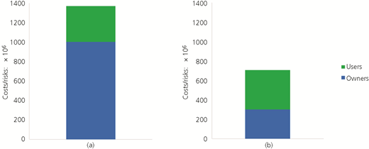
In order to have managers understand why specific intervention strategies should be followed, they need to be able to see what effect their decision makes on the stakeholders. They need to be able to do this for the whole time period being investigated (Figures 2–4) and at smaller intervals within that time period (Figure 5). Once this is clear, it is useful to show the values of the proxies for the whole time period and at smaller intervals within that time period. The costs and proxies are shown in the following two sections and the referenced appendices.
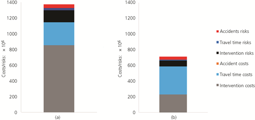
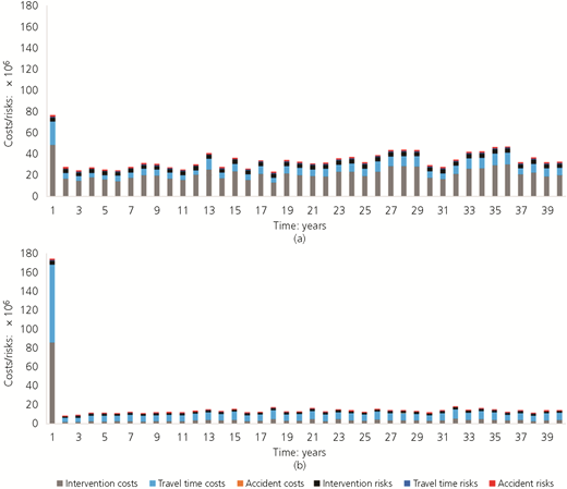
Total costs/risks per cost/risk type per year: (a) strategy set 1; (b) strategy set 2
Total costs/risks per cost/risk type per year: (a) strategy set 1; (b) strategy set 2
Cost and risks
In order for managers to understand the effects of their decisions, they need to be able to make a number of comparisons. The usefulness of comparisons using all objects is summarised in Table 18. The usefulness of comparisons using objects of one type is summarised in Table 19.
Usefulness of comparisons using all objects over the entire time period
| Comparison for different strategy sets … | Allows statements … | Example | |
|---|---|---|---|
| 1 | … Of the total costs/risks | … Of which in general is better | The total costs/risks of strategy set 2 (€303 × 106) are lower than the total costs/risks of strategy set 1 (€1005 × 106); therefore, it is clear that one should choose the strategies with earlier preventive interventions – that is, do not neglect maintenance (Table 20) |
| 2 | … Of the costs/risks per stakeholder | … As to how each stakeholder is affected and enables discussions about trade-offs between stakeholders | The owner should be willing to execute more on later but better preventive interventions, such as renewal interventions when objects are in state 4 – that is, strategy set 1 should be followed instead of strategy set 2 – to reduce the user costs/risks (€368 × 106 against €407 × 106) (Table 20) |
| 3 | … Of the costs/risks per period of time | … As to how each stakeholder is affected and enables discussions about trade-offs between the frequency and extent of interventions of different types | The owner should be willing to spend more on earlier preventive interventions such as rehabilitation interventions when objects are in state 3 – that is, strategy set 2 should be followed instead of strategy set 1 – to reduce the risks for all stakeholders (€226 × 106 against €125 × 106) (Table 20) |
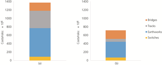
| 4 | … Of the costs/risks per object type that causes them | … As to where efforts should be focused to reduce costs | The largest sources of costs/risks are tracks (€51 × 106 if strategy set 2 is followed) and earthworks (€79 × 106 if strategy set 1 is followed and €16 × 106 if strategy set 2 is followed) (Table 21) |
Usefulness of comparisons using all objects in each year
| Comparison for different strategy sets … | Allows … | Example | |
|---|---|---|---|
| 5 | … Of the total costs/risks | … General statements of which is better | Although the total costs/risks of strategy set 2 are lower than the total costs/risks of strategy set 1 over the entire period, they are substantially higher in year 1 (€176 × 106 against €78 × 106). The costs/risks from years 2 to 40 are, however, reversed (<€20 × 106/year against <€60 × 106/year) (Figure 5) |
| 6 | … Of the costs/risks per stakeholder | … Statements as to how each stakeholder is affected and enables discussions about trade-offs between stakeholders | The owner should be willing to pay more on preventive interventions than the lowest amount in year 1 – that is, €50 × 106 when following strategy set 1 against €82 × 106 when following strategy set 2 for interventions in year 1 (Figure 5) – so that there are reduced user risks over the entire time period (€75 × 106 against €50 × 106 (Table 20)) |
| 7 | … Of the costs/risks per period of time | … Statements as to how each stakeholder is affected and enables discussions about trade-offs between the frequency and extent of interventions of different types | The owner should be willing to pay more on preventive interventions than the lowest amount in year 1 – that is, €50 × 106 when following strategy set 1 against €82 × 106 when following strategy set 2 for interventions in year 1 (Figure 5) – so that costs of corrective interventions – that is, intervention risk is lower over the entire time period (€151 × 106 against €75 × 106 (Table 20) |
| 8 | … Of the costs/risks per object type that causes them | … Statements as to where efforts should be focused to reduced costs | The largest sources of costs/risks in year 1 are tracks (€103 × 106 and €51 × 106 if strategy sets 1 and 2 are followed) and earthworks (€79 × 106 if strategy set 1 is followed and €16 × 106 if strategy set 2 is followed) (Table 21) |
Total costs and risks
| Stakeholder | Label | Costs/risks | Estimation | Total costs/risks: € × 106 | |
|---|---|---|---|---|---|
| Strategy set 1 | Strategy set 2 | ||||
| Ownera | Intervention | Costs | 854 | 228 | |
| Risks | 151 | 75 | |||
| Total intervention costs/risks | 1005 | 303 | |||
| Total owner costs/risks | 1005 | 303 | |||
| Users | Travel time | Costs | 293 | 357 | |
| Risks | 30 | 10 | |||
| Total travel time costs/risks | 323 | 367 | |||
| Accident | Costs | 0 | 0 | ||
| Risks | 45 | 40 | |||
| Total accident costs/risks | 45 | 40 | |||
| Total user costs/risks | 368 | 407 | |||
The owner costs of intervention for all objects are €854 billion with strategy 1 and €228 million with strategy 2 over a network of c. 211 km for 40 years, which translate into average annual costs per kilometre of c. €101 127 and €27 032, respectively. This is in agreement with the average cost per annual maintenance of railway infrastructure in Europe by Jimenez-Redondo et al. (2012) (€30 000–100 000/(km year))
Total costs/risks per object type
| Object type | Strategy set 1: € × 106 | Strategy set 2: € × 106 | |||||
|---|---|---|---|---|---|---|---|
| Costs | Risks | Total | Costs | Risks | Total | ||
| Bridge | Metal | 25 | 3 | 28 | 35 | 1 | 36 |
| Concrete | 4 | <1 | 5 | 2 | <1 | 2 | |
| Masonry | 160 | <1 | 161 | 162 | <1 | 162 | |
| Total | 190 | 4 | 193 | 199 | 1 | 200 | |
| Track | Total | 309 | 103 | 412 | 18 | 51 | 68 |
| Earthwork | Embankment | 178 | 30 | 207 | 103 | 7 | 111 |
| Cutting | 422 | 50 | 472 | 251 | 8 | 260 | |
| Total | 600 | 79 | 679 | 355 | 16 | 370 | |
| Switch | Total | 48 | 40 | 89 | 14 | 57 | 71 |
| Total | 1147 | 226 | 1373 | 585 | 125 | 710 | |
Proxies
When proxies for what matters are requested, they need to be displayed well. The displays for the proxies are shown for the entire time period in Figures 6–9. The usefulness of comparisons using all objects is summarised in Table 22.
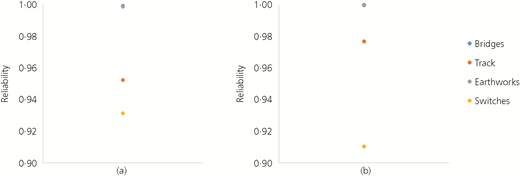
Average reliability of the objects in all years: (a) strategy set 1; (b) strategy set 2 (the switches are less reliable with intervention strategy 2 than with intervention strategy 1 because although there are fewer switches in state 5, there are more that are not in state 1)
Average reliability of the objects in all years: (a) strategy set 1; (b) strategy set 2 (the switches are less reliable with intervention strategy 2 than with intervention strategy 1 because although there are fewer switches in state 5, there are more that are not in state 1)
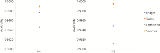
Average availability of the objects in all years: (a) strategy set 1; (b) strategy set 2 (there is lower availability due to bridges and earthworks when following intervention strategy 2 than when following intervention strategy 1 because there are more preventive interventions executed that take considerable amounts of time)
Average availability of the objects in all years: (a) strategy set 1; (b) strategy set 2 (there is lower availability due to bridges and earthworks when following intervention strategy 2 than when following intervention strategy 1 because there are more preventive interventions executed that take considerable amounts of time)
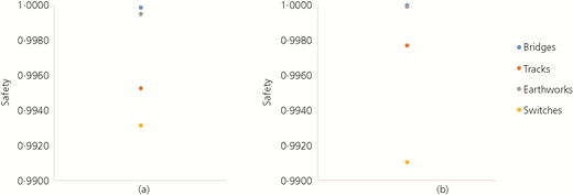
Average safety related to all objects in all years: (a) strategy set 1; (b) strategy set 2 (safety due to the switches decrease when intervention strategy 2 is followed compared to when intervention strategy 1 is followed because although there are fewer switches in state 5, there are more that are not in state 1)
Average safety related to all objects in all years: (a) strategy set 1; (b) strategy set 2 (safety due to the switches decrease when intervention strategy 2 is followed compared to when intervention strategy 1 is followed because although there are fewer switches in state 5, there are more that are not in state 1)
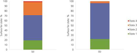
Average state of all objects over time period: (a) strategy set 1; (b) strategy set 2
Average state of all objects over time period: (a) strategy set 1; (b) strategy set 2
An overview of the proxies
| Proxy | Allows statements related to the | Example |
|---|---|---|
| Reliability | Probability of not providing the expected level of service | The illustration of the average reliability of the bridges, tracks, earthworks and switches (0·995, 0·9525, 0·9987 and 0·9314 with strategy 1 and 0·999, 0·9768, 0·9997 and 0·9103 with strategy 2) gives an indication of how likely it is that a failure might happen. Figure 6 gives an indication that if strategy set 2 is followed, the railway network will be more reliable than if strategy set 1 is followed; however, it can be seen that this is not the case for objects of all types. There is, however, no information as to how much one should spend to remedy this or who is predominantly affected by this |
| Availability | Amount of time that railway objects are likely to not provide the expected level of service | The illustration of the average availability of the bridges, tracks, earthworks and switches (0·9997, 0·9990, 0·9946 and 0·9988 with strategy 1 and 0·9948, 0·9996, 0·9997 and 0·9994 with strategy 2) gives an indication of how long objects will be working as intended. It can be seen (Figure 7) that if strategy set 2 is followed, the railway objects will be providing the expected level of service for more time than if strategy set 1 is followed. There is, however, no information as to how much one should spend to remedy this or who is predominantly affected by this |
| Safety | Probability of users being injured or losing their lives | The illustration of the average probability of being injured or killed due to an accident on a bridge, track, earthwork and switch (0·9998, 0·9952, 0·9995 and 0·9931 with strategy 1 and 1·0000, 0·9977, 0·9999 and 0·9910 with strategy 2) enables one to see (Figure 8) that following strategy set 1 will result in far fewer injuries or fatalities than following strategy set 2. This allows discussion as to how much one should spend to prevent accidents. It does not, however, enable the full picture |
| State | The improvement or deterioration of the objects | The illustration of state gives an overall approximate view of whether or not the infrastructure is getting worse and the probability that it will fail (Figure 9). It also gives an idea of the amount of money one will need to spend in the future. It is, however, meaningful only if one compares it to an optimal trajectory of the state over time |
Discussion
The results show that there is a difference between showing the costs related to providing an adequate level of service and not providing an adequate level of service to all stakeholders and using proxies. If the costs are used alone, one can see how each of the stakeholders is likely to be affected over the period of time being investigated. If the proxies are used alone, one can zero in on a few items that may be of particular interest to someone in an infrastructure management organisation, but it is difficult to come to a defendable decision as to which interventions should be executed on the infrastructure network. Basically, using costs enables engineers and managers to speak with each other. They show how the technical issues contained in the intervention strategies translate into the ability of the manager to ensure that his infrastructure provides an adequate level of service. Of course, there are likely many situations in which the use of proxies to emphasise what is happening in parts of the system in addition to costs will be useful, particularly if engineers or managers are used to using them.
The proposed approach may be described as a multicriteria decision analysis approach, in that it takes into consideration all criteria that are important in a system when estimating and communicating maintenance needs. A significant difference of this approach from many other multicriteria decision analysis approaches, however, is that the use of explicit weights is avoided – that is, there is no weight put on an accident and no weight put on the cost of intervention. Instead, it is proposed to place a value on how stakeholders are affected per unit time – that is, the probability of having an accident multiplied by the costs of the accident, which includes, for example, having stakeholders assign a value to an injured person and a lost life. Along these lines it is noted that the proposed approach helps to ensure that all stakeholders and how they are affected is taking into consideration and that the valuations of the impacts on stakeholders is given in directly comparable units. This is important in most situations, but particularly important in potentially controversial situations – for example, when a manager and an engineer work for different entities.
Despite all of the advantages of the proposed approach, there are numerous challenges when implementing it. These are listed as follows:.
It is more time intensive than basing arguments on technical aspects, as it requires first being aware of the technical aspects and then converting them to service.
It is not always easy to identify all of the aspects of service that one would like to value and put values on the units of them in meaningful ways. For example, how does one value the aesthetics of a bridge in a railway network when it is like new and when it is in a deteriorated state?
It is not easy to take into consideration widely different valuations of one unit of service between stakeholders and to estimate how these values change over time as a function of changing state of infrastructure. For example, a reduction of noise for 1 h may be worth a large amount to one stakeholder but may not be worth anything to another and the estimate of the difference in accident risk when a train is going over track in state 2 and state 3 might be challenging.
Conclusion
As shown in this paper, engineers and managers, with the use of the proposed approach, can, with a little effort, speak to each other. The key to this successful communication is to focus on providing the required level of service and to show clearly how technical issues can affect the provided level of service. Once arguments are made from the service point of view, then, and only then, does it make sense to investigate clearly defined proxies, such as risk, reliability, availability and safety. As this is true regardless of the infrastructure analysed or the methodology or techniques used, the proposed approach is suitable for use with many if not all of the methodologies used today, together with many, if not all, of the different asset management work prioritisation and appraisal tools used in the industry. The proposed approach, although intuitive, is one that has not yet been proposed in literature in the field of infrastructure asset management.
With the rigorous application of this approach, engineers are going to increase their ability to convince managers that they should spend more on maintenance when it is justified, and managers are going to increase their ability to explain to engineers why they are not spending on maintenance when it is not justified. To explore exactly the extent of these improvements, however, more research is required. Three example research topics are as follows
comparison of the use of building an argument for maintenance spending on an infrastructure networks using this approach against using others – for example, approaches based only on technical aspects, only on partial service indicators or on partial assessments of service
investigation of the ability of stakeholders to determine a unified definition of the service provided by infrastructure for specific types of infrastructure, their ability to place values on them and their ability to accept that interventions were not necessarily being executed when they thought they should, of which the latter may lead to stakeholders insisting on the ability to enter constraints in the optimisation models or insisting that specific interventions were to be executed regardless of the optimisation
investigation of the benefits of using this approach to develop the next generation of documents aimed at reporting on infrastructure to managers, politicians and the public (e.g. Asce, 2017; SBB-Infrastruktur, 2016); considerable effort goes into developing these documents currently, but the results are not normally informative enough to help decision makers objectively determine required maintenance funding levels.
Acknowledgement
This work has received funding from the European’s Union Horizon 2020 research and innovation programme under grand agreement number 636285 (Destination Rail project).
