


Railways are critical infrastructure systems because their construction, use, operation, maintenance and development affect multiple stakeholders within society. To ensure that these systems function as intended over time, railway managers execute interventions. Railway managers are interested in determining which interventions to execute by considering the trade-offs between the intervention costs and effects on service consistently and transparently. Currently, however, this is not possible, because existing methodologies use qualitative indicators instead of quantifying the rail service directly. This paper shows how the direct quantification of the effects on rail service per unit time enables interventions to be selected by making optimal trade-offs between intervention costs and effects on service when the acceptable service levels are respected. The usefulness of direct quantification is demonstrated by comparing two sets of intervention strategies for the track, switches and bridges of an example network for 30 years, by using direct estimates of service and four service indicators, state, reliability, availability and safety. As railway management moves from qualitative to quantitative and data-driven decision-making, the direct quantification of the effects on service provides a more informative way to compare intervention strategies than the use of service indicators.
Notation
- A
average availability
availability of asset i in nominal state s
- Ccor
cost of corrective interventions
cost of corrective interventions on asset i in nominal state s
- CDAP.a
accident costs for the directly affected public
accident costs for the directly affected public due to failure of asset i in nominal state s
- CIAP.a
accident costs for the indirectly affected public
accident costs for the indirectly affected public due to failure of asset i in nominal state s
- CIAP.env
environmental costs for the indirectly affected public
- CIAP.env/f
environmental costs for the indirectly affected public due to failure, including corrective interventions
environmental costs for indirectly affected public due to failure, including corrective interventions, of asset i in nominal state s
environmental costs for the indirectly affected public due to interventions on asset i in nominal state s
- CIAP.env/pr
environmental costs for the indirectly affected public due to preventive interventions
environmental costs for the indirectly affected public due to preventive interventions on asset i in nominal state s
- Cpass.a
accident costs for passengers
accident costs for passengers due to failure of asset i in nominal state s
- Cpass.d
delay costs for passengers
- Cpass.d/f
delay costs for passengers due to failure, including corrective interventions
delay costs for passengers due to failure, including corrective interventions, of asset i in nominal state s
delay costs for passengers due to interventions on asset i in nominal state s
- Cpass.d/pr
delay costs for passengers due to preventive interventions
delay costs for passengers due to preventive interventions on asset i in nominal state s
- Cpr
cost of preventive interventions
cost of preventive interventions on asset i in nominal state s
- df-i
delay minutes per day of traffic disruption due to failure, including corrective interventions, of asset i
- dpr-i
delay minutes per day of traffic disruption due to preventive intervention on asset i
- ei
extent of asset i
length of asset i
extent of asset i in the state s in year t
- i
asset
- la-i
lateral distance affected per accident per unit of the length of asset i
- NDAP
average population per square metre of the affected area
- Npass
average number of passengers per train
- Pa-i
probability of an accident occurring per failure of asset i
- PDAP.fat-i
probability of fatality per accident per person in the affected area due to failure of asset i
- PDAP.inj-i
probability of injury per accident per person in the affected area due to failure of asset i
probability of failure of asset i in nominal state s
- Ppass.fat-i
probability of fatality per accident per passenger in train due to failure of asset i
- Ppass.inj-i
probability of injury per passenger in train due to failure of asset i
- R
average reliability
reliability of asset i in nominal state s
nominal state of asset i in year t
- Sw
average weighted state
weighted state of asset i in year t
- Saf
average safety
safety of asset i in nominal state s
- s
state or nominal state
- tf-o
duration of traffic disruption due to failure of asset i
duration of traffic disruption due to the execution of preventive intervention type prt on asset i
- uccor-i
unit cost of corrective intervention on asset i
- ucDAP.fat
unit cost of a directly involved public fatality
- ucDAP.inj
unit cost of a directly involved public injury
- ucd
unit cost of delays
- ucenv.f-i
unit cost of environmental preservation impacts due to failure, including corrective interventions, of asset i
unit cost of environmental preservation impacts due to preventive intervention type pt on asset i
- ucIAP.fat
unit cost of a fatality for indirectly involved public
- ucIAP.inj
unit cost of an injury for indirectly involved public
- ucpass.fat
unit cost of a passenger fatality
- ucpass.inj
unit cost of a passenger injury
unit cost of preventive intervention type pt on asset i
Introduction
As the state of the rail infrastructure deteriorates over time, its ability to provide service decreases. According to the EU standard EN 50126 on railway applications, often referred to as Rams (reliability, availability, maintainability and safety), functional states are used to describe changes in service provision and are defined using criteria related to the context of the infrastructure – for example, physical, social, legislative and commercial factors (NEN, 1999). The lowest functional state of infrastructure is often referred to as the critical state, and it is the lowest acceptable state. The state of the infrastructure can be improved with the execution of interventions. An intervention on the infrastructure can be either corrective or preventive (Innotrack, 2010). When a failure occurs, a corrective intervention is executed to restore the service provided by the infrastructure, while preventive interventions are executed based on prescribed criteria to reduce the probability of infrastructure failure (NEN, 1999). A preventive intervention must always be executed before the infrastructure deteriorates beyond the critical state to ensure acceptable service levels.
A manager may decide to execute a preventive intervention before the critical state is reached for numerous reasons – for example, to increase the service provided by the infrastructure, to extend the lifetime of the asset, to avoid the execution of a more extensive intervention at the critical state or to reduce the effects on service due to the execution of the more extensive intervention. Another critical reason to execute a preventive intervention before the asset reaches its critical state is to reduce its probability of failure. Even when an asset has a probability of failure below the allowable levels, a manager should still consider this probability and the efficient options to reduce it further. These are long-term considerations of the trade-offs between the intervention costs and the service provided by the asset with and without the execution of the intervention. However, managers can also decide to change the timing of a preventive intervention by considering short-term trade-offs between the intervention costs and the service provided by a network due to different planning of work zones – for example, grouping interventions in space and time to reduce the effects on service. The long-term planning of all interventions to be executed on an asset by considering the many possible states of this asset leads in the establishment of intervention strategies. The implementation of an intervention strategy affects the required budget for both preventive and corrective interventions and how service is likely to be provided in the future. The short-term planning of interventions based on externalities, such as the states of other assets within the same network or other assets in other networks, is part of the constructing of an intervention programme (Adey, 2019). This work focuses on intervention strategies and specifically on the usefulness of directly quantifying the effects on service over time instead of using service indicators to compare intervention strategies.
Most methodologies used to determine the intervention strategies for rail infrastructure use either the intervention costs over the lifetime of a single asset – that is, life-cycle costs – and/or one or more service indicators – for example, reliability and availability (Innotrack, 2009a). Such service indicators are also described in the standard EN 50126 – for example, the number of expected failures, expected delay hours, mean time to repair and expected number of accidents. Although these methodologies are better than simply using expert opinion to determine when an intervention should be executed, they do not allow for direct comparisons with the intervention costs. For example, if intervention strategies A and B have the same intervention costs but strategy A results in a lower probability of accident occurrence and a longer mean time to repair than strategy B, which strategy should be selected?
Three other problems often occur with the use of service indicators according to current methodologies.
Indicators are selected based on experience, creating inconsistencies between the assessment of intervention strategies performed by different experts (Nyström and Söderholm, 2010) and railway authorities (Innotrack, 2009a).
Tools and service indicators are developed with explicit focus on specific asset types, and therefore, their use cannot be easily transferred to different asset types – for example, in the paper by Miwa and Mizuno (2014), derailments are used as a service indicator to plan interventions on track, but this service indicator cannot be easily used to assess interventions on bridges.
Important effects on service are often neglected because commonly used indicators do not cover them – for example, environmental impacts of interventions (Bouch and Roberts, 2010; Fracchia et al., 2012).
By quantifying and monetising the effects of interventions instead of using service indicators, it is possible to allow for direct comparisons between the different effects of interventions on the service – for example, delays and environmental impacts – and between the effects of interventions and intervention costs. Hence, the monetisation of effects on service due to interventions is used in life-cycle cost analysis (Zoeteman, 2001), and it can be used together with cost–benefit analysis to assess intervention strategies. However, in railway management, this approach has been developed only for assessing intervention strategies for a single asset type by monetising only a single type of effect – for example, delays (Zoeteman, 2004) and accidents (Ioannidou and Pyrgidis, 2014). Consequently, in railway management, there has been little work quantifying and monetising the multiple effects of service when assessing intervention strategies, and to the authors’ knowledge, there has not been any work that presents how this could be implemented in a systematic way and across different railway asset types.
This paper shows how the systematic quantification of multiple effects on service per unit time can be used to compare intervention strategies consistently across different railway asset types. The improvement is demonstrated by comparing two sets of intervention strategies for the track sections, switches and bridges of an example network for 30 years, first by quantifying service per unit time and then using the four commonly used service indicators, state, reliability, availability and safety. All intervention costs and effects on service are quantified per unit time and monetised.
The remainder of this paper is divided as follows. The section headed ‘Literature review’ contains a review of the literature on the evaluation of intervention strategies for railway assets. The section headed ‘Example’ presents the example network and the two candidate strategies. The section headed ‘Results’ shows the estimation of intervention costs for the example infrastructure. The assessment of the effects on service using two methods – that is, quantification of the effects on service and service indicators – is presented in the section headed ‘Building arguments for strategy sets’. The sections headed ‘Discussion’ and ‘Conclusions’ contain the discussion and conclusions.
Literature review
In recent years, many decision support models and tools have been developed to help railway managers plan maintenance on the infrastructure. Most research has been focused on deterioration and maintenance planning for different types of railway assets. For example, in the paper by Soleimanmeigouni et al. (2018), reviews of the deterioration and maintenance models for the ballasted track are presented. Many studies have also focused on the integration of deterioration and maintenance modelling in a decision support tool. These tools aim to predict the state of an infrastructure asset in the future and suggest the optimal time for an intervention to be executed. Usually, an objective function is used to determine at which stage of the deterioration curve a preventive intervention should be executed. Such tools can be used to determine and compare intervention strategies. The objective function in these tools is often the minimisation of intervention costs and/or maximisation/minimisation of one or several other measures of service (Patra, 2009).
When intervention costs are considered, the tools estimate the costs of either preventive or preventive and corrective interventions for a time period or the lifetime of the asset. This is achieved by considering different preventive interventions to be executed at different time intervals or different states of the asset. The tools can then select the strategy that results in the minimum costs. Examples of such tools are Ecotrack (Rivier, 1998); RI-AMS (Jovanovic and Zoeteman, 2010); the tools presented by Caetano and Teixeira (2015), Putallaz and Rivier (2004), Grimes and Barkan (2006), Beck et al. (2008), Meier-Hirmer et al. (2009), Nissen (2009a), Kim et al. (2010), Silmon and Roberts (2010), Strataki (2011) and Le and Andrews (2013); and the many tools used by national railways in Europe, reviewed by Innotrack (2009b). These tools can estimate the intervention costs and the expected state of the infrastructure when an intervention strategy is implemented for a specific time period. However, these tools do not consider other effects on the rail service such as delays caused by rerouting or train cancellations due to the unavailability of the infrastructure during the execution of the corrective or preventive interventions, although according to the standard ISO 55000 on asset management (ISO, 2014), the standard EN 50126 and EU regulations such as those by the European Community (EC, 2007, 2016) and Community of European Railway and Infrastructure Companies (CER, 2012), not only the intervention costs but also all relevant effects on all stakeholders should be considered.
Such effects on the rail service are considered by tools that use one or more service indicators. These service indicators are included in the objective function to assess the effects of different interventions and schedules on the rail service. The standard EN 50126 suggests many such service indicators. The tools that use service indicators can be divided into two main groups, the tools that use qualitative service indicators and the tools that use quantitative service indicators. A commonly used qualitative indicator is the state of the infrastructure. By estimating the average state of the infrastructure over time due to the implementation of different intervention strategies, it is possible to compare their performance. Examples of these tools for the track are Ramsys (Jovanovic, 2006), the Petri net model presented by Andrews et al. (2014), the Markov model presented by Prescott and Andrews (2015) and the adaptive neural-network-based fuzzy inference system presented by Dell’Orco et al. (2008). Although these tools are capable of accurately modelling the behaviour of the specific asset type for which they were developed, they often cannot be used to assess intervention strategies across different asset types consistently. Additionally, they do not yield to quantitative estimates of the effects on service, and therefore, they cannot be used to assess if an improvement in the value of a service indicator is beneficial when considering the intervention costs required to achieve it. For example, one cannot definitively argue that an intervention strategy that results over the next 30 years in a 1% improvement of the average state of an asset and 50% additional intervention costs should be implemented.
The tools that use quantitative service indicators estimate proxies of the service, such as reliability, availability, maintainability and safety, or specific impact indicators, such as number of failures, number of delays, number of interventions and number of accidents. For example, in the paper by Rhayma et al. (2013), reliability is used to determine the optimal intervention strategy for the track. In the paper by Zhao et al. (2007), reliability is used to identify the best intervention strategy for sleepers. In the paper by Macchi et al. (2012), the best intervention strategy for networks consisting of track sections, switches and the trackside signalling system is determined using reliability targets. In the paper by Rama and Andrews (2013), the reliability of switches is estimated to be used in the development of optimal intervention strategies. In the publications by Song and Schnieder (2018), Quiroga and Schnieder (2010) and Winther et al. (2015), the availability is used as a service indicator to evaluate interventions. Often accidents and safety-related service indicators are used when maintenance on rail, switches and level crossings is assessed. For example, in the paper by Zhao et al. (2006), the number of derailments is used as a service indicator, while in the paper by Ćirović and Pamučar (2013), safety – that is, the probability of an accident occurring – is used as a service indicator to determine the optimal level crossing configuration. Although these tools are capable of assessing different intervention strategies, due to their explicit focus on one service indicator, other substantial effects related to the execution of interventions are neglected.
Some tools have been developed to consider multiple service indicators. For example, in the paper by Andrews (2013), both the number of expected closures due to failures and the number of preventive interventions are considered, and in the paper by Morant et al. (2016), reliability, availability and safety are estimated using a data-driven decision support model to determine the optimal intervention strategy for the signalling system. Bemment et al. (2018) analysed the reliability and availability of switches based on historical data failures. These approaches provide railway managers with a broader overview of the effects related to maintenance decisions. However, when using these tools to compare different intervention strategies, it is often the case that one strategy performs better than another strategy for a group of service indicators but not for all. To overcome this, some tools consider multiple service indicators in one objective function using, for example, multi-criteria analysis – for example, the studies by Connolly and O’Connor (2017), Su et al. (2017) and Núñez et al. (2019). These tools can integrate many effects related to intervention strategies into a single value that can be directly used in the selection of the optimal intervention strategy. The values of the service indicators, however, have different units compared with intervention costs, which makes it impossible to compare directly an improvement on the objective function with the intervention costs required to achieve this improvement (Adey et al., 2019).
In 2008, the EU recognised the need to quantify the effects of transport services by using monetised values to help railway managers to make rational maintenance decisions (Maibach et al., 2008) based on cost–benefit analysis (Boardman et al., 2017). Additionally, many studies have been conducted in Europe, in China and in the USA to determine unit cost values for a broad range of effects related to the rail service – for example, the studies by Kalivoda et al. (2003), Grimes and Barkan (2006), Axhausen et al. (2008), Beck et al. (2008), Nash et al. (2009), Nissen (2009b), van Essen et al. (2011), International Union of Railways (UIC, (2012), Korzhenevych et al. (2014) and EC (2014).
A small number of studies have used this information in the quantification of the effects related to interventions in monetised units and therefore comparable values. Ioannidou and Pyrgidis (2014) and Pyrgidis et al. (2016) quantified the different effects related to interventions on level crossings to decide which interventions result in the least overall cost. These studies, however, often focus on one asset type, and therefore, there are inconsistencies between the effects that are quantified for different asset types.
Papathanasiou et al. (2019) proposed to quantifying all services provided per unit time that affect all stakeholders when planning interventions on railway networks. Although they gave an extensive definition of the railway service – that is, a function of how every stakeholder is affected by the changes in the state of the railway infrastructure and a description of the effects related to all stakeholders due to changes in the service – they stopped short of demonstrating how this definition could be used to determine the best intervention strategies for assets of multiple types and therefore of demonstrating that their definition is better than using service indicators.
Example
Infrastructure
The usefulness of the quantification of the effects on service per unit time is demonstrated by evaluating two sets of intervention strategies for all of the railway assets in a part of the railway network in Dublin, Ireland (Figure 1). More than three-quarters of the length of the network is built on bridges. This part of the network serves only passenger trains and consists of 5164 m of the track, divided into 11 track sections (based on the location of stations and signals), 23 switches and 39 bridges with a total deck surface area of 16 763 m2. The track sections and bridges are further divided into subtypes, based on their structural and operational characteristics (Table 1).
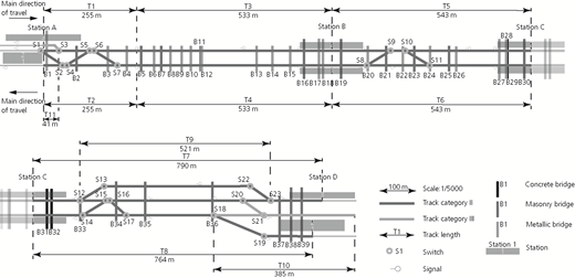
Infrastructure assets of the example network
Infrastructure assets of the example network
Number and extent of the assets per asset types and subtypes
| Asset type | Asset subtypes | Description | Number of assets | Total extent of assets | Unit of measure |
|---|---|---|---|---|---|
| Track sections | Track category I | Track sections on lines where there is a 160 km/h maximum line speed | 0 | 0 | m of length |
| Track category II | Track sections on lines where there is between 40 and 160 km/h maximum line speed | 9 | 4738 | ||
| Track category III | Track sections on lines where there is lower than 40 km/h maximum line speed | 2 | 426 | ||
| Total | 11 | 5164 | |||
| Switches | — | All switches | 23 | 23 | Number of assets |
| Bridges | Concrete | Bridges whose primary construction material is concrete | 3 | 592 | m2 of deck surface area |
| Masonry | Bridges whose primary construction material is masonry | 17 | 7319 | ||
| Metallic | Bridges whose primary construction material is metal | 19 | 8852 | ||
| Total | 39 | 16 763 | |||
States
It is assumed that each asset can be in one of four possible functional states, state 1: excellent – that is, no observable structural damages; state 2: good – that is, first appearance of minor but yet noticeable structural damages; state 3: acceptable – that is, significant structural damages but adequate stability; and state 4: poor – that is, potential lack of structural stability. State 4 is the last functional state of an asset, and therefore, it is the critical state – that is, an intervention should always be executed when an asset reaches this state to ensure acceptable service levels. The states of the assets in year 1 are shown in Figure 2.
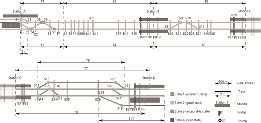
State of assets in the first year, year 1
State of assets in the first year, year 1
Deterioration
The deterioration of the assets over time is modelled by estimating the probability of the asset being in each state over time and (Equations 1 and 2). The probabilities of transitioning between states in two consecutive years for each asset type are given in Table 10 in the Appendix.
Intervention strategies
Two sets of intervention strategies are considered (Table 2). Strategy set A contains major preventive interventions that are executed only when assets are in state 4. Strategy set B contains minor preventive interventions when assets are in state 3 and major preventive interventions when assets are in state 4. As state 4 is the critical state of the assets, both strategy sets fulfil the minimal requirement for the service – that is, a major preventive intervention is to be executed when assets reach the critical state. However, strategy set A does not include any additional preventive interventions compared with the minimum requirement, while strategy set B includes an additional minor preventive intervention at state 3. Preventive interventions are considered to improve the state of the asset (Table 11). The strategy sets include corrective interventions that are triggered by the failure of an asset, which can occur in each year as a function of a state-dependent probability (Table 10). Corrective interventions are assumed to restore the asset to its prior-to-failure state immediately.
Costs of preventive and corrective interventions
It is assumed that preventive interventions are executed at the end of the year in which the nominal state of the asset exceeds the trigger intervention state and according to each strategy (Table 2). The corrective interventions are executed each year as a function of the probability of the asset to fail, which in turn is a function of the nominal state. The costs of a preventive intervention are given by Equation 3, where the preventive intervention unit costs for the two preventive intervention types – that is, minor and major – are given in Table 11 and the extent of the assets is given in Table 9.
The costs due to failure, including the costs of corrective interventions, are given by Equation 4, where is the probability of failure, given the nominal state of the asset (Table 10) and uccor-i is the corrective intervention unit cost (Table 12).
Effects on service
The quantification of an effect on service is done by determining how the following are affected: (a) the passengers – that is, persons who use the infrastructure to travel; (b) the directly affected public – that is, persons other than users who are in the vicinity of the railway but not using it; and (c) the indirectly affected public – that is, persons who are neither users nor in the vicinity of the railway but are affected by it. How each stakeholder may be affected is shown in Table 3, which is a subset of the service measures proposed by Papathanasiou et al. (2019). This subset includes only state-dependent service measures.
Estimation of effects on service
| Stakeholder | Cost category | Description | Estimated by |
|---|---|---|---|
| Passengers | Accident | Economic impact of property damage and societal impact of injuries and fatalities due to accidents that involve passengers | |
| Delays | Economic impact of delays related to the infrastructure | ||
| Directly affected public (DAP) | Accident | Economic impact of property damage and societal impact of injuries and fatalities due to accidents that involve the directly affect public | |
| Indirectly affected public (IAP) | Accident | Economic impact of injuries and fatalities | |
| Environmental preservation | Environmental impact of environmental pollution and climate change and cultural impact due to changes in the railway infrastructure |
The effects on service are estimated using the following assumptions.
The preventive interventions are planned. Thus, it was considered that they are executed during the weekends and holidays to minimise the traffic disruption. Their effect on delays was estimated based on the timetable set for weekends (Tables 9 and 11). The corrective interventions are executed immediately when a failure occurs to return the service to the acceptable levels, and therefore, they cannot be planned. It was considered more likely for a failure to occur during a weekday, as the stress on the infrastructure is higher compared with that on weekends, when the traffic is less. It was assumed that there is a probability of 0·70 for a failure to occur during a weekday and a probability of 0·30 to occur during a day of the weekend or holidays. Hence, the effect of the corrective interventions on delays was estimated based on the corresponding timetable (Tables 9 and 12).
If the asset fails, accidents might occur, leading to injuries and/or fatalities and corrective interventions according to the EC (2016).
The accidents result in costs for the passengers and people in the vicinity of the railway – that is, directly affected public (Table 12) – according to the EC (2016).
Due to the accidents directly affecting the passengers and people in the vicinity of the railway, the indirectly affected public incurs costs.
All interventions, preventive and corrective, cause delays (Tables 11 and 12) and environmental preservation impacts (Table 13). The probabilities of correlated failures are zero.
All passenger trains are supposed to travel through stations A, B, C and D according to the timetable of 2017 (Aksentijevic et al., 2017) as they would if all infrastructure assets were in state 1 – that is, it is only deviations from this service that are relevant in the planning of the interventions. It was considered that if trains could not travel between the stations of the network, based on this timetable and the layout of the network – that is, location of signals and switches – due to the unavailability of an asset, an alternative means of transport must be used – for example, by bus – and the delay of this trip was estimated.
The unit costs considered for the example are given in Table 14.
Service indicators
Four service indicators are selected to be used to compare the sets of intervention strategies, state, reliability, availability and safety. These four service indicators are defined to be state-dependent and, therefore, can be used to assess the effects on service due to preventive interventions and failures, such as delays and accidents. The four service indicators (Table 4) are estimated for the assets in the same example network.
Quantification of service using the service indicators of state, reliability, availability and safety
| Service indicator | Definition | Shown as | Equation/comment |
|---|---|---|---|
| State | The physical condition of the infrastructure | Weighted state of an asset by its extent per year | Based on deterioration when no preventive interventions are executed (Table 10) and on the weighted state after interventions when preventive interventions are executed (Table 11) |
| Reliability | The probability that an item can perform a required function under given conditions for a given time interval (NEN, 1999) | Reliability of each asset per year | Based on the probability of failure of each asset (Table 10) |
| Availability | The ability of a product to be in a state to perform a required function under given conditions at a given instant of time or over a given time interval assuming that the required external resources are provided (NEN, 1999) | Availability of each asset per year | Based on the interruption of traffic due to preventive (Table 11) and corrective (Table 12) interventions and the extent of each asset |
| Safety | Freedom from unacceptable risk of harm (NEN, 1999) | Probability of accidents to occur due to failures of an asset per year | Based on the probability of an accident to occur due to the failure of each asset (Table 10) |
Results
General
In order to investigate the usefulness of the quantification of the effects on service per unit time, the two sets of intervention strategies were evaluated using (a) the intervention costs, (b) the effects on service and (c) the service indicator values. The investigated time period was 30 years. Discounting was not considered. The results of the simulations using the information in the section headed ‘Example’ are presented in the following subsections by providing summary tables or figures and stating the main observations. This information is used in the section headed ‘Building arguments for strategy sets’ to illustrate the usefulness of the direct quantification of service as opposed to using service indicators.
Intervention costs
Table 5 shows the intervention costs per asset type and strategy set. The following can be seen.
Strategy set A has higher total intervention costs than strategy set B.
Strategy set A has lower preventive and higher corrective intervention costs than strategy set B.
Among all the asset types, bridges are the main cost drivers in both strategy sets.
Intervention costs per asset type and strategy set over the 30-year period
| Asset type | Number of and costs per type of preventive interventions: € millions | Costs due to corrective interventions: € millions | Total intervention cost: € millions | ||||||
|---|---|---|---|---|---|---|---|---|---|
| Type | Number | C pr | C cor | C pr + C cor | |||||
| A | B | A | B | A | B | A | B | ||
| Track | Minor | 0 | 19 | 0 | 0·07 | 1·89 | 0·89 | 2·57 | 0·95 |
| Major | 2 | 0 | 0·68 | 0 | |||||
| Switches | Minor | 0 | 46 | 0 | 0·46 | 5·52 | 2·81 | 14·72 | 3·27 |
| Major | 23 | 0 | 9·20 | 0 | |||||
| Bridges | Minor | 0 | 33 | 0 | 30·75 | 1·71 | 0·55 | 15·55 | 41·74 |
| Major | 4 | 3 | 13·84 | 10·44 | |||||
| All assets | 29 | 101 | 23·72 | 41·72 | 9·12 | 4·24 | 32·84 | 45·96 | |
Figure 3 shows the preventive and corrective intervention costs per asset type, strategy set and year. The sum of the intervention costs for all the assets of each strategy set was used along with the effects on rail service or service indicators to assess the implementation of each strategy. The following can be seen.
Strategy set A has more peaks – that is, more years when the costs are significantly higher than the average annual costs due to the execution of 26 additional major preventive interventions (two on track, 23 on switches and one on bridges), compared with strategy set B.
Strategy set B has the highest costs in a year, for two consecutive years, year 22 and year 23, due to the execution of 33 minor preventive interventions on bridges.
Preventive interventions are the main driver of the costs in every year.
Both strategy sets have almost equally high intervention costs in year 1 mainly due to three major preventive interventions on bridges.
For both strategy sets, the average corrective intervention costs per year are lower than the preventive intervention costs.
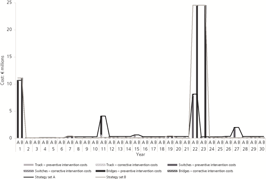
Intervention costs per asset type, strategy set and year
Intervention costs per asset type, strategy set and year
Effects on service
Table 6 shows the effects on service per asset type and strategy set. The following can be seen.
Strategy set B has lower effects on service than strategy set A.
Strategy set B has lower effects on delays and accidents but higher effects of environmental preservation than strategy set A.
Among all the asset types, switches cause the most effects in both strategies.
Among all the effects on service, accidents cause the highest effects on service, mainly due to switch failures.
Effects on service per asset type and strategy set over the 30-year period
| Asset type | Effects on service due to: € millions | Total effects on service: € millions | ||||||||||
|---|---|---|---|---|---|---|---|---|---|---|---|---|
| Preventive interventions | Failure, including corrective interventions | |||||||||||
| Delays | Environmental preservation | Accidents | Delays | Environmental preservation | ||||||||
| A | B | A | B | A | B | A | B | A | B | A | B | |
| Track | 0·002 | 0·02 | 0·02 | 0·1 | 405 | 189 | 0·2 | 0·1 | 0·2 | 0·1 | 405 | 189 |
| Switches | 2 | 0·2 | 0·01 | 0·01 | 726 | 369 | 7 | 3 | 0·02 | 0·01 | 735 | 373 |
| Bridges | 55 | 312 | 0·1 | 2 | 167 | 49 | 25 | 8 | 0·02 | 0·01 | 247 | 370 |
| All assets | 57 | 312 | 0·1 | 2 | 1229 | 582 | 32 | 11 | 0·13 | 2 | 1318 | 909 |
Figure 4 shows the accident costs due to failures and the delay and environmental preservation costs due to both preventive interventions and failures per asset type, strategy set and year. The sum of these costs for all the assets over the 30-year time period of each strategy is the total effects on rail service due to the implementation of each strategy. The following can be seen.
Strategy set A has lower effects than strategy set B for the majority of years.
Strategy set A has lower accident costs but higher delay costs than strategy set B for all the years.
Among all effects on service, accident costs are the most significant for the majority of the years for both strategies.
Delay costs due to preventive interventions in strategy set B in years 22 and 23 are the driver of the highest effects in service in a time unit.
For both strategy sets, the environmental preservation impacts are not significant compared with the rest of the effects on service.
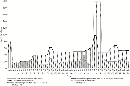
Effects on service per asset type and strategy set and year
Effects on service per asset type and strategy set and year
Service indicators
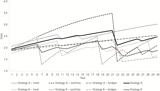
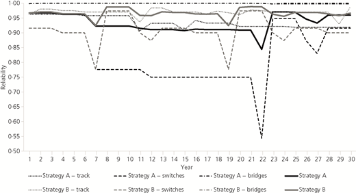
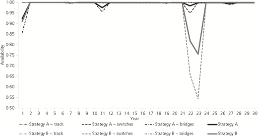
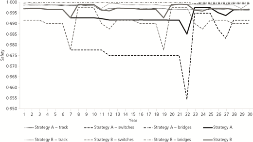
Table 7 shows the average state, reliability, availability and safety of all assets over the investigated 30-year time period. The following can be seen.
Strategy set B results in a better average state than strategy set A.
Strategy set A results in more reliable assets than strategy set B.
Strategy set A results in slightly higher availability of assets than strategy set B.
Strategy set B results in slightly safer assets than strategy set A.
Bridges have the highest average state, reliability and safety but the lowest availability compared with switches and tracks in both strategies.
Switches have the lowest reliability and safety compared with track and bridges in both strategies.
Service indicators related to the effects on service per intervention strategy set over the 30-year period
| Asset type | Average over 30 years | |||||||
|---|---|---|---|---|---|---|---|---|
| State S w | Reliability R | Availability A | Safety Saf | |||||
| A | B | A | B | A | B | A | B | |
| Track | 2·555 | 1·990 | 0·936 | 0·970 | 1·000 | 1·000 | 0·997 | 0·999 |
| Switches | 2·525 | 1·979 | 0·822 | 0·910 | 1·000 | 1·000 | 0·982 | 0·991 |
| Bridges | 2·219 | 1·944 | 0·999 | 1·000 | 0·999 | 0·997 | 1·000 | 1·000 |
| All assets | 2·366 | 1·962 | 0·934 | 0·967 | 0·999 | 0·998 | 0·994 | 0·997 |
Figures 5–8 show the state, reliability, availability and safety of the assets per asset type, strategy and year. The average value of each service indicator over all the assets in the network was also estimated for each year. The average value of each service indicator of the 30-year period for each intervention strategy was used to assess the effects on rail service related to the implementation of each strategy.
Weighted state per asset type, strategy set and year
Weighted state per asset type, strategy set and year
Reliability per asset type, strategy set and year
Reliability per asset type, strategy set and year
Availability per asset type, strategy set and year
Availability per asset type, strategy set and year
Safety per asset type, strategy set and year
Safety per asset type, strategy set and year
It can be seen that although there are the same correlations between the service indicators for all asset types, these correlations are not equally significant for all the asset types. For example, for all the assets with the improvement in the state, reliability and safety are also improved and availability is negatively affected. This pattern is pronounced for switches but not for bridges. The improvement in the state of bridges causes a significant drop in availability, but it only slightly improves reliability and safety.
Building arguments for strategy sets
General
In this section, arguments are made for strategy sets A and B. This is done by first building an argument for the best strategy set using intervention costs and the effects on service for strategy sets A and B (see the section headed ‘Intervention costs and effects on service’), then building an argument for the best strategy using the intervention costs and service indicators for strategy sets A and B (see the section headed ‘Intervention costs and service indicators’) and then comparing the two methods of comparison in terms of their usability (see the section headed ‘Usability’) and their ability to make decisions (see the section headed ‘Ability to make decisions’).
It is important to note that the implementation of either strategy set A or strategy set B was considered to fulfil the minimum requirements for the service set by factors such as physical, social, legislative and commercial.
Intervention costs and effects on service
The results of the estimations of intervention costs and the quantification of the effects on service show that for this example, strategy set B is better than strategy set A because its implementation results in €409 million fewer effects on service (Table 6) with a comparatively moderate increase in intervention costs – that is €13 million more intervention costs (Table 5). Table 8 shows the intervention costs and effects on service per asset type and strategy. The following can be seen.
Strategy set B has lower total intervention costs and effects on service than strategy set A.
Strategy set A has lower costs and effects due to preventive interventions but significantly higher costs and effects due to failure and corrective interventions than strategy set B.
Strategy B is better than strategy A when it is applied on track and switches, but strategy A performs better than strategy B when it is applied on bridges.
Intervention costs and effects on service per asset type and strategy set over the 30-year period
| Asset type | Interventions and effects on service due to: € millions | |||||
|---|---|---|---|---|---|---|
| Preventive interventions | Failure, including corrective interventions | Sum of preventive interventions and failure, including corrective interventions | ||||
| A | B | A | B | A | B | |
| Track | 0·70 | 0·22 | 406·82 | 189·81 | 407·52 | 190·03 |
| Switches | 10·75 | 0·67 | 738·51 | 375·67 | 749·26 | 376·33 |
| Bridges | 69·07 | 354·52 | 193·58 | 57·24 | 262·65 | 411·77 |
| All assets | 222·50 | 408·80 | 1270·79 | 599·14 | 1493·28 | 1007·94 |
Figure 9 shows the intervention costs and effects on service per asset type, strategy set and year. The following can be seen.
The sum of the costs and effects for all the assets is higher when strategy set A is followed than when strategy set B is followed in almost every year of the 30-year period.
Strategy B on bridges in years 22 and 23 causes high intervention costs and high delay costs due to the execution of preventive interventions.
Strategy set A for switches and track causes higher accident costs than strategy set B after year 8.
Strategy A for bridges results in higher accident costs than strategy B after year 23.
In the majority of the years and for both strategy sets, the accidents due to failures of switches and track have the highest costs compared with all intervention costs and other effects on service.
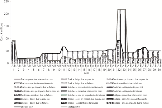
Costs and effects on service per asset type, strategy set and year
Costs and effects on service per asset type, strategy set and year
Additional observations can be made when the distribution of costs and effects between the stakeholders is examined. If the owner of the infrastructure is responsible for the execution of interventions and therefore for the intervention costs, then all the intervention costs and effects on service can be assigned to a stakeholder – that is, the cost for the owner is considered equal to the sum of the intervention costs (C pr + C cor).
Figure 10 shows the intervention costs and effects on service per stakeholder, strategy set and year. The following can be seen.
The owner is affected more by strategy set B, mainly in years 22 and 23, than by strategy set A.
Although the passengers are affected significantly in years 22 and 23 by strategy set B, for the majority of the years, they are affected less by strategy set A than by strategy set B.
The directly affected public incurs significantly higher costs by strategy set A than by strategy set B, mainly after year 8.
The indirectly affected public is affected every year more by strategy set A than by strategy set B.
Almost every year and for both strategies, passengers and the directly affected public are the two stakeholders who are affected the most.
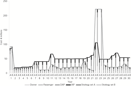
Costs and effects on service per stakeholder, strategy set and year
Costs and effects on service per stakeholder, strategy set and year
Intervention costs and service indicators
Using intervention costs and the four service indicators alone, it is not possible to know which strategy set is the best. Strategy B requires €13 million more to be spent on interventions (Table 5), and it results in higher average state, reliability and safety but lower average availability compared with strategy set B (Table 7). To decide whether strategy set B is better than strategy set A, one should further examine whether it is worth investing 33% additional budget on interventions to achieve 19% better overall state, 3% higher reliability, 0·3% higher safety and yet 0·1% less availability.
By considering the intervention costs (Table 5) and the four service indicators per asset type (Table 7), the following can be seen.
Strategy B, when implemented on track, results in 92% higher intervention costs, 24% better state, 3% higher reliability and 0·2% higher safety compared with strategy A. Availability differs insignificantly between the two strategies – that is, 0·01% – when they are applied on track.
Strategy B, when implemented on switches, results in 127% higher intervention costs, 24% better state, 10% higher reliability and 0·9% better safety compared with strategy A. Availability differs insignificantly between the two strategies – that is, 0·02% – when they are applied on switches.
Strategy B, when implemented on bridges, results in 91% higher intervention costs, 13% better state and 0·1% higher reliability but 0·2% lower availability compared with strategy A. Safety differs insignificantly between the two strategies – that is, 0·01% – when they are applied on bridges.
Usability
When comparing intervention strategies, quantifying the effects on service requires significantly more resources – that is, data, time and expertise – in addition to the resources required for the estimation of the intervention costs compared with the use of service indicators. Quantifying the effects on service per unit time required the monetisation of the effects on service per unit time. This quantification requires the estimation of several parameters in addition to the parameters required for the estimation of the intervention costs. Service indicators may require only the estimation of a few additional parameters. Regarding the example presented here and the ease of use, it can be seen that in addition to the data used for the estimation of the intervention costs, it was required
to estimate many variables to quantify the effects on service – for example, the probability of a fatality to occur given an accident, the probability of an injury to occur given an accident, the affected population in the vicinity of the railway per accident, the number of cancelled trains per hour of traffic disruption hour and the amount of carbon dioxide (CO2) emissions per intervention and many unit costs – for example, the unit cost per fatality, per injury or per minute of delay
to estimate the duration of traffic disruption per intervention and the probability of an accident to occur given a failure, to estimate the service indicators.
Ability to make decisions
Currently, intervention strategies can be assessed consistently for assets of different types over time using either intervention costs and the effects on service or intervention costs and service indicators. However, by quantifying the effects on service instead of using service indicators, more informed decisions can be made. The consideration of the information required for the quantification of the effects on service is more detailed, resulting in more accurate evaluation of the strategies and, therefore, more informed decisions. This is demonstrated in the example in many ways. For example, regarding the availability and the effects on service due to delays
The availability considers only the downtime of an asset due to both preventive interventions and failures resulting in corrective interventions but not the timetable. Hence, when the same intervention is executed on two assets with the same extent, the same availability was estimated, independently of their use according to the timetable.
The effects on service due to delays consider the downtime of an asset due to both preventive interventions and failures resulting in corrective interventions, the number of delays and lost trips caused due to the unavailability of the asset according to the timetable and the unit cost of delays for passengers. This means that when the same intervention is executed on two assets with the same extent, the effects on service due to delays were varied based on their use according to the timetable.
Not only do the two methods require a different amount of data, but they also produce different types of results that may affect their use in decision-making. By quantifying the effects on service using the same units with the intervention costs, the results are directly comparable. This helps to decide conclusively which intervention strategy should be applied and defend this decision by demonstrating which intervention strategy has an overall better outcome, when both the effects on service and intervention costs are considered. This is not always the case when service indicators are used to assess intervention strategies because the results might not allow for direct comparisons between the values of different service indicators and between the values of service indicators and intervention costs. The ability to make a conclusive decision on which strategy to implement is demonstrated in the presented example using the two methods.
Service indicators did not give conclusive results on whether one strategy is better than the other. Strategy A resulted in higher network availability, while strategy B gave better results for the average state, reliability and safety of the assets (Table 7). An evaluation of whether strategy A is better than strategy B could not be made based on the estimation of these service indicators alone, as their values are not comparable.
The consideration of service indicators together with intervention costs did not give a definite answer as to whether the average state, reliability and safety achieved by following strategy set B (Table 7) are worth the higher intervention costs (Table 5).
Using effects on service together with intervention costs gave a conclusive answer to which strategy is the best among the two – that is, strategy set B results in lower overall costs, including intervention costs and effects on service, compared with strategy A (Table 8).
When using intervention costs and effects on service, it was evident that the improvements in service following the strategies in set B (Table 6) are worth the higher intervention costs (Table 5).
Although the use of any common scale or any utility function produces comparable values for the intervention costs and the effects on service and therefore helps make a conclusive decision, the use of monetary units as a common scale makes the process more transparent. By using monetary values to quantify the effects on service, an individual is more likely to perceive the differences in the scale due to their familiarity with the metric. Individuals are more likely to understand differences in monetary values intuitively – for example, between €1 and 100 – than differences in the values of service indicators – for example, between 0·98 and 0·99 for availability – or in the values of an objective or utility function. Hence, stakeholders are more likely to understand the results of the strategy set comparison when the effects of service are quantified and monetised, which makes the decision-making process more transparent. The ability to make a transparent decision based on intuitively perceived results is demonstrated in the presented example using the two methods.
The service indicators of reliability, availability and safety were all estimated using probabilities. When strategy set B is implemented instead of strategy set A, reliability and safety were increased by 3·5 and 0·3%, respectively, while availability was reduced by 0·1% (based on the results for all assets given in Table 7). However, a non-expert might not be able to judge if the higher values of reliability and safety achieved by strategy set B have significant benefits over the values of reliability and safety provided by strategy set A and how these benefits are related to the benefits of the higher availability provided by strategy set A compared with the availability provided by strategy set B.
The monetisation of the effects on service provided an intuitive comparison between the effects of the strategy sets. When strategy set B is implemented instead of strategy set A, the effects due to accidents were reduced by 50%, while the effects due to delays and environmental preservation were increased by 263 and 1640% (based on the results for all assets given in Table 6). However, strategy set B is better compared with strategy set A because the reduction in the effects due to accidents achieved by strategy set B has a much higher impact, equal to €643 million, compared with the increase in the effects due to delays and environmental preservation, which is equal to €238 million (based on the results for all assets given in Table 6).
Moreover, the stakeholders can be involved in the process, which helps in making objective decisions that are more likely to be accepted. For example, they can be involved in a consultation process to determine which effects should be quantified and which models should be used and to examine whether all the relevant effects on service were considered in the analysis adequately. Additionally, stakeholders and managers can make more informed decisions. For example, they can decide to implement the option with the least accidents, even if this solution does not result in the lowest overall intervention costs and effects on service. In this case, by quantifying the effects on service, it is possible to provide clarity on how and to which degree each stakeholder is likely affected by this option, which enables an open discussion between the stakeholders and increases the objectivity of the decision-making process and the acceptance of its results. The use of service indicators does not provide the same transparent view of the effects of intervention strategies to the stakeholders. For example, if the stakeholders want to choose the option with the highest safety, they cannot have a tangible value for this option’s impact on the availability, judging only by the value of this service indicator.
Discussion
In this paper, it is shown that the use of intervention costs and quantified effects on service per unit time helps in making conclusive and more transparent decisions on intervention strategy implementation for each asset type, than by using the traditional approach of intervention costs and service indicators. A few areas of the existing work that might provide an even stronger argument are discussed in this section.
Only three effects on service – namely, delays, accidents and environmental preservation impacts – and four service indicators – namely, state, reliability, availability and safety – were used in the example. Other effects on service – for example, as suggested by Papathanasiou et al. (2019) – and other service indicators – for example, as suggested by EN 50126 or Innotrack (2009a) – could be used. Although these may render the example more complete in some ways, they would not improve the illustration that quantified effects on service per unit time provide the base for a more informative comparison of intervention strategies when used together with intervention costs than by using intervention costs and service indicators.
The effects on service were monetised to convert them into units that were directly comparable with intervention costs. Other approaches also exist to quantifying the effects of service in values comparable with the intervention cost – for example, using a utility. The use of utility might be, in some ways, more correct. However, when a utility is used instead of monetised units, the already easily comprehensible unit costs of interventions are converted into something that is, at best, not intuitive for railway managers and stakeholders. Although the use of another standard unit instead of monetary units can be proposed – for example, using a multi-criteria decision analysis with an objective function – it is unlikely that managers and stakeholders will be as familiar with another scale as they are with monetary units.
In the example, it was assumed that each asset fails independently of the rest of the assets in the network and that each intervention is executed on one asset at a time. This is an oversimplification of reality. Often multiple assets fail simultaneously, which increases the probability of accidents to occurring and the number of delays. Additionally, when an intervention strategy is implemented, multiple interventions can be executed simultaneously, in an intervention programme, to reduce the effects caused by preventive interventions (Burkhalter and Adey, 2018). If the implementation of the intervention strategies had been considered for multiple assets or more complex rules were used to convert the results of the intervention strategies into intervention programmes, the example would produce more realistic results. For example, a manager should consider executing the preventive intervention on bridges between two stations in the same period in order to minimise the effects related to delays. With such considerations, it would be possible to produce more realistic and reliable estimates of the intervention costs, the effects on service and the service indicators in order to optimise an intervention strategy. However, this would not take away from the argument that by quantifying effects on service per unit time, railway managers can produce more informed assessments of intervention strategies.
Only two sets of simple intervention strategies were used in the example, and the implementation of either strategy set fulfils the minimum service requirements for this network. These intervention strategies and this assumption greatly simplify the actual intervention planning problems faced by railway managers. The majority of the intervention planning problems faced by the railway managers would require more complicated analyses to be performed to make a decision. However, even considering the simple intervention planning problem presented in the example, the use of service indicators did not provide a definitive solution on which strategy set is the best, while the quantification of the effects on service provides a conclusive answer. Hence, although the two methods were applied in this paper to provide an answer to a simplified problem, the drawn conclusions on the usability and the ability to make decisions are expected to be applied even when more realistic, complicated planning problems are examined.
The estimation of intervention costs, the monetisation of the effects on service and the calculation of the service indicators was done in this paper using data specific to the considered assets and data based on expert opinion and sources in the literature. The paper does not explain in detail how these values were calculated. Hence, it provides only limited information to those either attempting to reproduce the numbers or attempting to do so for other railway assets. Nevertheless, a detailed explanation of the calculations made for this example would not improve the illustration that by quantifying the effects on service per unit, values comparable with the intervention costs can be produced, which has a substantial advantage over the use of intervention costs with service indicators when comparing intervention strategies.
The uncertainties associated with the estimation of the values used in the example – for example, evolution of asset state over time, the probabilities of failure, unit costs of interventions, unit costs of the effects on service – are not discussed explicitly in this paper. Such information would be beneficial if the purpose of the paper was to give a detailed explanation of how the effects of intervention strategies should be modelled over time. Although such work would provide an insight into the accuracy of the modelling, it would add to the discussion of whether it is useful to quantify the effects on service per unit time instead of estimating service indicators, when comparing intervention strategies for which the intervention costs are known.
Despite the benefits of the quantification of the effects on service in making informative decisions, there are some shortcomings related to its implementation in practice. The higher number of variables required to quantify the effects on service and their uncertainty make it harder for a railway manager to implement this method for intervention strategy evaluation, instead of using service indicators. Although all the input data required for such a comparison are related to uncertainties of different degrees, many of the variables required for the quantification of the effects on service are related to particularly high uncertainties – for example, the probability of a fatality occurring given an accident and the affected population in the vicinity of the railway per accident. These high uncertainties should be quantified to produce reliable results. This process requires even more data and resources. For many railway managers, acquiring all the data required for the quantification of both the effects on service and the uncertainty of the results might be a deterring factor in implementing this method.
On the contrary, the lower data requirements of service indicator estimation might be seen as a simpler and therefore better option. However, as railway management moves from qualitative to quantitative asset management, it becomes necessary to make data-driven decisions and to utilise existing knowledge, experience, information and data sets. It should be, therefore, preferred to consider all relevant information regarding the effects on service – for example, consulting experts and determining ranges of values – over excluding important factors from the assessments – for example, the number of delays due to unavailability of an asset, the impacts of an accident due to a failure of an asset and the consumption in environmental resources due to the execution of an intervention. Including those factors in the decision-making sets the foundation of improving their estimation methods and the collection of data required for their estimation. Already, many applications in railways utilise big data analytics (van Gulijk et al., 2015), and many railway agencies are investing in digitisation to leverage on existing information and data (Johansson et al., 2019). Thus, although the quantification of the effects on service might be seen as not aligned with current practices because it requires more data than the use of service indicators, it capitalises on digitisation and it is aligned with the requirement to move towards data-driven decision-making in railway management.
Conclusions
Current methodologies used to determine the intervention strategies for railway infrastructure do so in ways in which the effects on service are not directly comparable with intervention costs. This is because they often rely on service indicators – for example, the state, reliability, availability and safety of infrastructure – instead of quantifying the service directly. This paper shows how the quantification of the effects on rail service per unit time, instead of service indicators, enables the determination of the best intervention strategy, in a way that makes it transparent to stakeholders why and under which conditions an intervention strategy is better than another. The usefulness of the proposed approach is demonstrated by comparing two sets of intervention strategies for the track sections, switches and bridges of an example network for 30 years, first by quantifying service per unit time and then by using the four service indicators, state, reliability, availability and safety. It is shown that the quantification of the effects on service per unit time provided a conclusive way to select the best intervention strategy, while the use of service indicators could not provide a definitive answer.
This paper demonstrates that although the quantification of the effects on service per unit time considers more data and therefore requires more resources, it is a more informative way to make decisions when comparing intervention strategies than the use of service indicators. To increase the impact of this work, it should be expanded to an even more realistic example. This should include more effects on service; explicit consideration of the variation in values used to estimate the effects on services due to changes in time and space – for example, timetable changes – the uncertainty associated with accidents; effect of deterioration and interventions on the state of infrastructure assets; more realistic intervention strategies; more realistic conversions from strategies to programmes; and modelling simultaneous failures and interventions.
Acknowledgements
The work presented here has received funding from Horizon 2020, the EU’s Framework Programme for Research and Innovation for the Destination Rail project under grant agreement 636285 and for the Foresee project under grant agreement 769373.
Appendix
In the following tables, the information used in the example for the estimation of the intervention costs, the effects on service and the service indicators is provided.
Asset-specific information
| Assets | Extenta | Length:b m | Delay minutes per day of traffic disruption due to | Asset | Extenta | Lengthb | Delay minutes per day of traffic disruption due to | ||||
|---|---|---|---|---|---|---|---|---|---|---|---|
| Preventive intervention | Failurec | Preventive intervention | Failurec | ||||||||
| e i | d pr-i | d f-i | e i | d pr-i | d f-i | ||||||
| Track sections | T1 | 255 | 255 | 85 234 | 481 424 | Bridges | B1 | 720 | 72 | 462 896 | 1 159 038 |
| T2 | 255 | 255 | 85 234 | 481 424 | B2 | 1130 | 113 | 462 896 | 1 159 038 | ||
| T3 | 533 | 533 | 30 860 | 131 854 | B3 | 470 | 47 | 462 896 | 1 159 038 | ||
| T4 | 533 | 533 | 30 860 | 131 854 | B4 | 320 | 32 | 462 896 | 1 159 038 | ||
| T5 | 543 | 543 | 76 918 | 192 456 | B5 | 372·4 | 38 | 462 896 | 1 159 038 | ||
| T6 | 543 | 543 | 76 918 | 192 456 | B6 | 166·6 | 17 | 462 896 | 1 159 038 | ||
| T7 | 764 | 764 | 49 662 | 135 292 | B7 | 166·6 | 17 | 462 896 | 1 159 038 | ||
| T8 | 790 | 790 | 49 662 | 135 292 | B8 | 350 | 35 | 462 896 | 1 159 038 | ||
| T9 | 521 | 521 | 0 | 0 | B9 | 500 | 50 | 462 896 | 1 159 038 | ||
| T10 | 385 | 385 | 29 797 | 81 173 | B10 | 250 | 25 | 462 896 | 1 159 038 | ||
| T11 | 41 | 41 | 0 | 0 | B11 | 350 | 35 | 462 896 | 1 159 038 | ||
| Switches | S1 | 1 | 10 | 85 234 | 481 424 | B12 | 1410 | 141 | 462 896 | 1 159 038 | |
| S2 | 1 | 10 | 85 234 | 481 424 | B13 | 500 | 50 | 462 896 | 1 159 038 | ||
| S3 | 1 | 10 | 85 234 | 481 424 | B14 | 450 | 45 | 462 896 | 1 159 038 | ||
| S4 | 1 | 10 | 85 234 | 481 424 | B15 | 400 | 40 | 462 896 | 1 159 038 | ||
| S5 | 1 | 10 | 85 234 | 481 424 | B16 | 640 | 64 | 462 896 | 1 159 038 | ||
| S6 | 1 | 10 | 85 234 | 481 424 | B17 | 230 | 23 | 462 896 | 1 159 038 | ||
| S7 | 1 | 10 | 85 234 | 481 424 | B18 | 230 | 23 | 462 896 | 1 159 038 | ||
| S8 | 1 | 10 | 76 918 | 192 456 | B19 | 960 | 96 | 462 896 | 1 159 038 | ||
| S9 | 1 | 10 | 76 918 | 192 456 | B20 | 320 | 32 | 461 510 | 1 154 716 | ||
| S10 | 1 | 10 | 76 918 | 192 456 | B21 | 600 | 60 | 461 510 | 1 154 716 | ||
| S11 | 1 | 10 | 76 918 | 192 456 | B22 | 330 | 33 | 461 510 | 1 154 716 | ||
| S12 | 1 | 10 | 49 662 | 135 292 | B23 | 460 | 46 | 461 510 | 1 154 716 | ||
| S13 | 1 | 10 | 49 662 | 0 | B24 | 450 | 45 | 461 510 | 1 154 716 | ||
| S14 | 1 | 10 | 49 662 | 135 292 | B25 | 650 | 65 | 461 510 | 1 154 716 | ||
| S15 | 1 | 10 | 49 662 | 135 292 | B26 | 720 | 72 | 461 510 | 1 154 716 | ||
| S16 | 1 | 10 | 49 662 | 135 292 | B27 | 270 | 27 | 461 510 | 1 154 716 | ||
| S17 | 1 | 10 | 49 662 | 135 292 | B28 | 765 | 45 | 461 510 | 1 154 716 | ||
| S18 | 1 | 10 | 49 662 | 135 292 | B29 | 192 | 12 | 461 510 | 1 154 716 | ||
| S19 | 1 | 10 | 49 662 | 135 292 | B30 | 110 | 11 | 461 510 | 1 154 716 | ||
| S20 | 1 | 10 | 49 662 | 135 292 | B31 | 160 | 10 | 461 510 | 1 154 716 | ||
| S21 | 1 | 10 | 49 662 | 81 173 | B32 | 240 | 15 | 461 510 | 1 154 716 | ||
| S22 | 1 | 10 | 49 662 | 0 | B33 | 345 | 15 | 297 972 | 811 750 | ||
| S23 | 1 | 10 | 49 662 | 135 292 | B34 | 345 | 15 | 297 972 | 811 750 | ||
| B35 | 136 | 8 | 297 972 | 811 750 | |||||||
| B36 | 425 | 25 | 297 972 | 811 750 | |||||||
| B37 | 187 | 11 | 297 972 | 811 750 | |||||||
| B38 | 187 | 11 | 297 972 | 811 750 | |||||||
| B39 | 255 | 15 | 297 972 | 811 750 | |||||||
The extent of the track sections is measured in metres of length and the extent of the bridges is measured in square metres of deck surface area
The length is the length of the track sections, the length of the switch configuration and the length of the bridges
The delays due to failure include the delays due to corrective interventions
State-specific probabilities
| Asset type | State | Transition probability per asset | Probability of failure per asset | ||||
|---|---|---|---|---|---|---|---|
| State at year t + 1 | |||||||
| 1 | 2 | 3 | 4 | ||||
| Track | Track category I | 1 | 0·98 | 0·02 | 0·00 | 0·00 | 0·003 |
| 2 | 0·00 | 0·93 | 0·07 | 0·00 | 0·025 | ||
| 3 | 0·00 | 0·00 | 0·80 | 0·20 | 0·075 | ||
| 4 | 0·00 | 0·00 | 0·00 | 1·00 | 0·25 | ||
| Track category II | 1 | 0·87 | 0·13 | 0·00 | 0·00 | 0·003 | |
| 2 | 0·00 | 0·95 | 0·05 | 0·00 | 0·028 | ||
| 3 | 0·00 | 0·00 | 0·93 | 0·07 | 0·09 | ||
| 4 | 0·00 | 0·00 | 0·00 | 1·00 | 0·28 | ||
| Track category III | 1 | 0·93 | 0·07 | 0·00 | 0·00 | 0·004 | |
| 2 | 0·00 | 0·97 | 0·03 | 0·00 | 0·036 | ||
| 3 | 0·00 | 0·00 | 0·95 | 0·05 | 0·11 | ||
| 4 | 0·00 | 0·00 | 0·00 | 1·00 | 0·36 | ||
| Switch | 1 | 0·79 | 0·21 | 0·00 | 0·00 | 0·01 | |
| 2 | 0·00 | 0·91 | 0·09 | 0·00 | 0·1 | ||
| 3 | 0·00 | 0·00 | 0·87 | 0·13 | 0·25 | ||
| 4 | 0·00 | 0·00 | 0·00 | 1·00 | 0·5 | ||
| Bridge | Concrete | 1 | 0·98 | 0·02 | 0·00 | 0·00 | 2·00 × 10−6 |
| 2 | 0·00 | 0·99 | 0·01 | 0·00 | 2·00 × 10−4 | ||
| 3 | 0·00 | 0·00 | 0·97 | 0·03 | 5·00 × 10−4 | ||
| 4 | 0·00 | 0·00 | 0·00 | 1·00 | 3·00 × 10−3 | ||
| Masonry | 1 | 0·97 | 0·03 | 0·00 | 0·00 | 4·00 × 10−8 | |
| 2 | 0·00 | 0·98 | 0·02 | 0·00 | 3·00 × 10−6 | ||
| 3 | 0·00 | 0·00 | 0·93 | 0·07 | 3·00 × 10−4 | ||
| 4 | 0·00 | 0·00 | 0·00 | 1·00 | 6·00 × 10−4 | ||
| Metal | 1 | 0·97 | 0·03 | 0·00 | 0·00 | 8·00 × 10−6 | |
| 2 | 0·00 | 0·98 | 0·02 | 0·00 | 3·00 × 10−4 | ||
| 3 | 0·00 | 0·00 | 0·95 | 0·05 | 5·00 × 10−3 | ||
| 4 | 0·00 | 0·00 | 0·00 | 1·00 | 5·00 × 10−2 | ||
Preventive intervention type-specific information
| Asset type | Preventive intervention type | State in which intervention can be executed | Probability of the asset being in each state following the intervention | Intervention costs: €/asset extent | Duration of traffic disruption: d/asset extent | ||||
|---|---|---|---|---|---|---|---|---|---|
| 1 | 2 | 3 | 4 | ||||||
| Track | Track category I | Minor | 3 | 0·8 | 0·2 | 0 | 0 | 7·5 | 0·0001 |
| Major | All | 1 | 0 | 0 | 0 | 750 | 0·0004 | ||
| Track category II | Minor | 3 | 0·7 | 0·3 | 0 | 0 | 7·5 | 0·0001 | |
| Major | All | 1 | 0 | 0 | 0 | 750 | 0·0004 | ||
| Track category II | Minor | 3 | 0·6 | 0·4 | 0 | 0 | 7·5 | 0·0001 | |
| Major | All | 1 | 0 | 0 | 0 | 750 | 0·0004 | ||
| Switch | Minor | 3 | 0·9 | 0·1 | 0 | 0 | 10 000 | 0·13 | |
| Major | All | 1 | 0 | 0 | 0 | 400 000 | 2 | ||
| Bridge | Concrete | Minor | 3 | 0·6 | 0·4 | 0 | 0 | 1000 | 0·06 |
| Major | All | 1 | 0 | 0 | 0 | 7500 | 0·12 | ||
| Masonry | Minor | 3 | 0·5 | 0·5 | 0 | 0 | 1000 | 0·08 | |
| Major | All | 1 | 0 | 0 | 0 | 8000 | 0·15 | ||
| Metal | Minor | 3 | 0·8 | 0·2 | 0 | 0 | 3000 | 0·08 | |
| Major | All | 1 | 0 | 0 | 0 | 5000 | 0·1 | ||
Asset type-specific information
| Asset type | Probabilities | Corrective intervention costs: €/asset extent | Duration of traffic disruption due to failure, including corrective interventions: d/asset extent | Lateral distance affected:a m | |||||
|---|---|---|---|---|---|---|---|---|---|
| Accident per failure | Fatality per accident per passenger | Injury per accident per passenger | Fatality per accident per person in the affected area | Injury per accident per person in the affected area | |||||
| P a-i | P pass.fat-i | P pass.inj-i | P DAP.fat-i | P DAP.inj-i | uccor-i | d f-i | l a-i | ||
| Track | Track cat. I | 0·1 | 0·05 | 0·4 | 0·075 | 0·05 | 200 | 0·0002 | 20 |
| Track cat. II | 0·05 | 0·025 | 0·2 | 0·0375 | 0·025 | 200 | 0·0002 | 20 | |
| Track cat. II | 0·01 | 0·003 | 0·02 | 0·0045 | 0·003 | 200 | 0·0002 | 20 | |
| Switch | 0·1 | 0·05 | 0·5 | 0·45 | 0·075 | 0·05 | 0·45 | 10 | |
| Bridge | Concrete | 0·2 | 0·2 | 0·8 | 0·3 | 0·2 | 3000 | 0·073 | 30 |
| Masonry | 0·25 | 0·2 | 0·8 | 0·3 | 0·2 | 2000 | 0·098 | 30 | |
| Metal | 0·3 | 0·2 | 0·8 | 0·3 | 0·2 | 4000 | 0·097 | 30 | |
Measured from the centre of the width of the asset
Environmental preservation impacts-specific information
| Asset type | Environmental preservation impacts due to: €/asset extent | |||
|---|---|---|---|---|
| Minor preventive intervention | Major preventive intervention | Failure, including corrective interventions | ||
| Track | Track category I | 15 | 21 | 19 |
| Track category II | 15 | 21 | 19 | |
| Track category II | 15 | 21 | 19 | |
| Switch | 155 | 215 | 192 | |
| Bridge | Concrete with length <250 m | 347 | 1155 | 809 |
| Concrete with length >250 m | 1155 | 1155 | 347 | |
| Masonry with length <250 m | 1155 | 504 | 1155 | |
| Masonry with length >250 m | 504 | 1155 | 1155 | |
| Metal with length <250 m | 1155 | 504 | 504 | |
| Metal with length >250 m | 504 | 1589 | 1155 | |
Variable-specific information
| Variable | Value | Unit | |
|---|---|---|---|
| Average number of passengers per train | N pass | 100 | Passengers/train |
| Average population per square metre of the affected area | N DAP | 75 | People/m2 |
| Unit cost of delays | ucd | 0·515 | €/delay minute |
| Unit cost of a passenger fatality | ucpass.fat | 1 500 000 | €/fatality |
| Unit cost of a passenger injury | ucpass.inj | 200 000 | €/injury |
| Unit cost of a directly involved public fatality | ucDAP.fat | 1 500 000 | €/fatality |
| Unit cost of a directly involved public injury | P DAP.inj-i | 200 000 | €/injury |
| Unit cost of a fatality for indirectly involved public | ucIAP.fat | 500 000 | €/fatality |
| Unit cost of an injury for indirectly involved public | ucIAP.inj | 100 000 | €/injury |

