
Determining how infrastructure corridors are to be designed optimally and modified over time is challenging due to the considerable uncertainty associated with potential changes in mobility patterns. This is due to factors such as the dynamisms of urban areas and the potential of transitioning to autonomous vehicles. Although currently this future uncertainty is taken into consideration in decisions with respect to highway designs and modifications in a qualitative manner, there is potential benefit to using quantitative methods and explicitly considering how highways may be modified in the future as a function of the actual future that emerges. In this paper, the use of a quantitative evaluation method using real options is explored to evaluate highway designs, considering uncertainties in future mobility patterns and management flexibility. The usefulness of the method is investigated on the fictive but realistic case study based on the completion of the A15 highway, in the canton of Zurich, Switzerland. The results of this exploratory work indicate significant value in the use of the proposed method to ensure that infrastructure networks are optimally prepared to support society in an unknown future, and it is expected that it can be used more extensively in future spatial planning.
Notation
- CAccident
accident costs
- CConstruction
construction costs
- CEnvironment
environmental costs
- CExtension/Adaption
extension or adaption costs of the highway
- CIntervention
intervention costs
- CMaintenance
maintenance costs
- CPopulation
costs of pollution per combustion engine vehicle user
- CTime
costs for lost time per user and hour
- CTot
total costs
- CTravel
travel costs
- CTravel time
costs of lost travel time
- DAV,t
percentage of autonomous vehicle users in year t
- DCV,t
percentage of combustion engine vehicle users in year t
- DEV,t
percentage of autonomous vehicle users in year t
- DNV,t
percentage of human-driven vehicle users in year t
- NAV
total number of autonomous vehicle users
- NCV,t
total number of combustion engine vehicle users
- NHomework,t
variability in users due to working from home in year t
- NInitial
number of users of the highway in year 0 – that is, at the completion of the construction
- NNV
total number of human-driven vehicle users
- NPopulation,t
number of additional users due to growth in population in year t
- NTrain,t
number of additional users due to the growth in the use of personal vehicles over trains in year t
- PAccident,AV
probability of occurrence of an autonomous vehicle accident
- PAccident,NV
probability of occurrence of a human-driven vehicle accident
- TLost,AV
lost time in year t per autonomous vehicle user in the highway
- TLost,NV
lost time in year t per human-driven vehicle user in the highway
- δt
delta Dirac function (δ t = 1 in the triggering year; δ t = 0 all other years)
Introduction
Highways are vital for the functioning of society, as they help ensure the safe and fast transport of persons and goods. If highways do not provide the expected level of service – for example, the ability to allow a vehicle to go from a point A to a point B in a specified amount of time – they are modified, which requires resources and causes disruptions to service. The ease with which a highway can be modified depends on its initial design, and although there are exceptions, the easier a highway is to modify, the more expensive it is to build. As the initial cost must be worth the gain in ease of modification – that is, flexibility – highway designs should be selected, taking into consideration both the possible future changes in required service levels and flexibility.
Possible traditional highway designs include (a) ‘myopic’ designs – that is, designs for the average expected traffic demand – that is, expected number of vehicles that need to travel on the highway – and (b) ‘robust’ designs – that is, designs for an above-average expected traffic demand. As predictions of the future are more often than not incorrect (Savage and Markowitz, 2009), designs based on the average expected traffic demand are, in most futures, suboptimal. To reduce the risk of making wrong predictions about the future, one may want to retain the option to modify the infrastructure depending on the development of contextual conditions (e.g. the traffic demand). The designer is therefore not constrained to choose only from myopic or robust designs. Similar to how Myers (1974) and Trigeorgis (1996) suggested, the retention of options to maximise the potential upsides and minimise the potential downsides of an investment in the financial industry, engineering structures can be designed so that options are retained to develop the infrastructure at a later time (de Neufville and Scholtes, 2011; Ellingham and Fawcett, 2007). For the evaluation of the design of non-spatially distributed infrastructure, the method of de Neufville and Scholtes (2011) has been used (Elvarsson et al., 2021; Martani et al., 2016).
In this paper, it is shown how one can consider future uncertainty and flexibility in the design of a new highway so as not to be constrained by myopic and robust designs. Consequently, the value of flexible infrastructure may prove to be better than that of traditional designs and ultimately lead to improved highway designs. The evaluation methodology is applied to a fictive but realistic case study based on the design of the A15 highway, between Uster and Junction Ottikon, in the canton of Zurich, Switzerland. In the example evaluation, it was considered that the future required service levels is uncertain due to the unknown future traffic demand both quantitatively – that is, the average number of vehicles that will be transiting on the highway in a day – and qualitatively – that is, the types of vehicles that will be transiting in terms of driving mode and propellant type.
The remainder of the paper is organised as follows. The section headed ‘Background’ contains a review of the state of the art of the research in the field. The section headed ‘A15 highway, between Uster and Ottikon’ contains the general description of the A15 highway. The section headed ‘Evaluation’ contains an example of how future uncertainty and flexibility can be used to move beyond myopic and robust designs. The section headed ‘Results’ shows, through the results, the potential increased value in considering future uncertainty and flexibility in designing highways. The sections headed ‘Discussion’ and ‘Conclusion’ contain the discussion and conclusions, as well as suggestions for future work.
Background
The evaluation of road designs, including those of highways, has included research on the use of multi-objective and multi-attribute analysis (examples are shown in Table 1, along with a description of the method used to conduct the analysis and whether or not possible future adaptations were considered) to optimise road design (e.g. to minimise economic and environmental costs) considering both constant traffic demand (Brauers et al., 2008; Tille and Dumont, 2003; Zavadskas et al., 2008) and variable traffic demand. (A generic multi-attribute analysis model generally can be described by the following components: (a) a set of objectives or attributes, (b) a set of feasible alternatives, (c) a number of decision constraints, (d) preference structure or weights and (e) a set of performance evaluations of alternatives for individual objectives or attributes (Zavadskas et al., 2008).) None of this research, however, considered the potential for further modifying the roads in the future. Examples of research where future modifications have been considered, albeit not for roads or other spatially distributed infrastructure, are shown in Table 2 along with the uncertain future trends considered and the simulation method used. Examples of research where flexibility has been considered in road management are shown in Table 3. However, these always refer to contractual flexibility with no considerations to possible modifications to the infrastructure.
Examples of research on the optimisation of road designs considering variable traffic demand but no possible future adaptation of the infrastructure
| Objective | Source | Tools and methods for decision optimisation |
|---|---|---|
| Maximise robustness of service in transportation network design under demand uncertainty | Ukkusuri et al. (2007) | A genetic algorithm to solve the robust network design problem |
| Maximise service reliability in network design | Sumalee et al. (2006) | A gradient-based optimisation algorithm is used to solve the reliable network design problem |
| Maximise accessibility in transportation network design | Di et al. (2018) | Monte Carlo simulations |
| Maximise both capacity reliability and travel time reliability | Chen et al. (2011) | Probability model |
| Maximise the network capacity | Yim et al. (2011) | Probability model |
| Maximise the expanded net present value of a network investment by optimising not only the design variables but also the timing of the investment decisions | Chow and Regan (2011) | Expected value model |
| Maximise the present expected system consumer surplus | Ukkusuri and Patil (2009) | Expected value model |
| Optimise road design to balance road pricing, traffic congestion and environmental costs | Li et al. (2012) | Monte Carlo simulations |
Examples of research considering future modifications
| Infrastructure | Source | Variability considered | Simulation method |
|---|---|---|---|
| Hospitals and clinics | de Neufville et al. (2008) | Patterns, causes and effects of health and disease, changes in medical technology | Monte Carlo |
| Esders (2017) | Change in the patient demand | Binomial trees | |
| Engineering systems for waste and energy | Cardin and Hu (2016) | Change in the required waste disposal capacity and energy supply | Monte Carlo |
| Bridges | Ellingham and Fawcett (2007) | Change in the traffic demand | Monte Carlo |
| Heating and cooling systems in office buildings | Martani et al. (2015, 2016) | Changes in the prices of gas and electricity, heating and cooling loadings and performance of the systems | Monte Carlo and Latin hypercube Monte Carlo |
| Building facades | Esders et al. (2016) | Changes in operating costs | Binomial trees |
| Buildings | Menassa (2011) | Changes in the performance of materials and components | Binomial trees |
| Military barracks | Esders et al. (2015) | Changes in the demand for space | Univariate random walk algorithms |
| Buildings | Fawcett and Chadwick (2007), Fawcett and Rigby (2009) | Change in the demand for working space | Agent-based simulation model |
| Building ground floors | Ellingham and Fawcett (2007) | Changes in commercial rents | Binomial trees |
| Office buildings | Gumaand de Neufville (2008) | Changes in rents and in the demand for office space | Monte Carlo |
| Ground-floor ceilings in buildings | Martani at al. (2018) | Change in the use of space | Monte Carlo |
| Buildings | Ashuri et al. (2011) | Change in the energy price | Binomial lattice and Monte Carlo |
| Multilevel parking facilities | de Neufville and Scholtes (2011), de Neufville et al. (2006) | Change in the number of parking plots required | Monte Carlo |
| Elvarsson et al. (2021) | Change in parking demand due to increase in shared automated vehicle deployment | Monte Carlo |
Examples of research considering contractual flexibility for the evaluation of road concessions
| Source | Variability considered | Simulation method |
|---|---|---|
| Galera and Soliño (2010) | Change in the traffic volume | Decision trees |
| Blank et al. (2016), Chiara et al. (2007), Shan et al. (2010), Soliño et al. (2018), Dong and Chiara (2010), Vasudevan et al. (2018) | Change in the traffic volume | Monte Carlo |
Although no examples have been found where flexibility has been used to design roads that could be adapted to cope with uncertain future conditions, many examples were found where contractual flexibility has been used in the evaluation of road concessions. In these cases, concessions were evaluated considering the uncertainty related to the future traffic volume, resulting in different combinations of minimum traffic guarantees and maximum traffic ceilings, and with implicit abandonment options (Blank et al., 2016). Examples of research where contractual flexibility was considered for road management are shown in Table 3.
It can be seen in both Tables 2 and 3 that the Monte Carlo method and binomial trees are two often-used simulation methods. Binomial trees are simple and transparent but not always representative of the future, because for most variables, there are more than two possible outcomes at every time step. Monte Carlo simulations are useful in modelling multivariate applications on both discrete and continuous scales (Brandimarte, 2014). Research has not yet been focused on the design of highways, or other spatially distributed infrastructure, taking into consideration future uncertainty in the mobility patterns and infrastructure flexibility.
A15 highway, between Uster and Ottikon
The object of investigation is the currently planned four-lane A15 highway section (Figure 1) between the Uster East junction and the Forchautostrasse at the Ottikon junction. This highway section will complete the A15 and in general improve the traffic flow in the surrounding area, particularly in Wetzikon and Hinwil. It will include a connection allowing fast entry to, and exit from, the highway to the west of Wetzikon, named Wetzikon West (Kantonsrat Zürich, 2020). The new highway section will be 8.2 km long, of which 4.5 km will be in tunnels. A bridge will be built enabling the highway to cross over the existing cantonal road in Aathal (Figure 1). On completion, traffic coming from the Zurich region and heading towards Chur will be redirected from its current path, which crosses multiple municipalities, to the highway. It is expected to reduce dramatically both the current and the future congestion on the roads of the involved municipalities. Exactly by how much it will help is, however, uncertain, due to (a) the uncertain spatial distribution of growth in the area (Kantonsrat Zürich, 2020); (b) the potential increase in the use of the home-office working mode following coronavirus disease 2019 (Covid-19); (c) advances in the auto industry, such as the emergence of autonomous vehicles and the conversion of vehicles from fossil to renewable sources (Bösch et al., 2018; Fagnant and Kockelman, 2015); and (d) changes in the modal split between private vehicles and public transport. Explicit consideration of these uncertainties in the design of the new highway section may result in an improved design over one that was either myopic or robust and in turn could result in a highway with increased societal benefits, lower costs or both. This requires building on the state-of-the-art methods used in Switzerland to account for the spatial effects of the transport infrastructures (ARE, 2007) and measuring the effects of traffic on the environment and land use (Astra, 2003; Fuhrer and Axhausen, 2018).
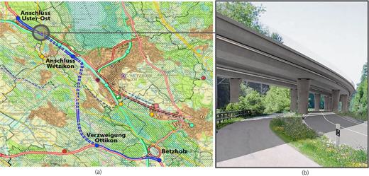
(a) Diagram of planned completion of the A15 highway (Kanton Zürich, 2019) with the tunnels marked with a dashed blue line, the open street sections with a continuous blue line and position of the new bridge in Aathal marked with a grey circle (‘Anschluss’ means ‘junction’, and ‘Verzweigung’ means ‘branching’); (b) a render of the planned bridge in Aathal (Redaktion Züriost, 2020)
(a) Diagram of planned completion of the A15 highway (Kanton Zürich, 2019) with the tunnels marked with a dashed blue line, the open street sections with a continuous blue line and position of the new bridge in Aathal marked with a grey circle (‘Anschluss’ means ‘junction’, and ‘Verzweigung’ means ‘branching’); (b) a render of the planned bridge in Aathal (Redaktion Züriost, 2020)
Evaluation
The steps used in this paper are similar to those used – for different infrastructures – in the studies by Esders et al. (2015) and Martani et al. (2016). They are as follows: (a) setting the boundaries, the interventions and the objective function to be used to determine the best highway design; (b) identifying the key uncertain variables to be modelled; (c) generating potential designs and how the highway would be modified to take into consideration multiple possible futures; (d) determining the values of the key variables that would result in modifications to the highways over time – that is, triggers – and (e) simulating what might happen in the future. These steps are explained in the following sections.
Boundaries, interventions and the objective of the evaluation
The effects of modifying highway networks can be extensive in both space and time. The spatial boundaries considered in this example were restricted to vehicles for the transport of both passengers (i.e. cars) and goods (i.e. trucks), travelling on the new highway section between the Uster East highway exit and Betzholz, in both directions. Vehicles were considered based on both their propellant mode (i.e. by both fuel combustion and electric (including hybrid) engines requiring charging) and driving mode (i.e. either human driven or autonomous). Effects on traffic flow on other regional roads (i.e. mainly on Aathalstrasse, Zürichstrasse and Rapperswilerstrasse) – for example, as a result of the vehicular flow transfer in case of traffic jams on the new highway section – were not considered. The time frame considered was 50 years following construction, and a rate of 3% was used to discount future cash flow, which is a common discount rate for infrastructure investments in many European countries (Mouter, 2018). After 50 years, no residual value of the infrastructure is accounted for. This is due to the fact that the future needs for the infrastructure are so uncertain that it is not considered worth assuming a residual value on the infrastructure as built at present.
The objective function used to decide which highway design yields the highest net benefit consists of the intervention costs and measures of service shown in Table 4. The value of each unit change in a measure of service is expressed in monetary values, as in the paper by Adey et al. (2020). It is given in the following equation:
where C Tot is the total costs, C Intervention is the total intervention costs over 50 years, C Travel is the total travel costs over 50 years and C Environment is the total environmental costs over 50 years.
Intervention costs and measures of service
| Type level 1 | Type level 2 | Unit values | Units |
|---|---|---|---|
| Cost of construction | Depends on the interventions; see Table 5 | — | |
| Cost of expansion | See Table 6 | — | |
| Cost of maintenancea | For roads | 5b | (CHF/m2)/year |
| For tunnels | 25b | (CHF/m2)/year | |
| For bridges | 35b | (CHF/m2)/year | |
| Travel time | 50c | (CHF/h)/vehicle | |
| Injuries | 320 000d | CHF/person | |
| Fatalities | 6 700 000e | CHF/person | |
| Property damages | 10 000f | CHF/vehicle | |
| Air pollution | 0.018g | (CHF/km)/CEV |
The cost of maintenance refers to the cost incurred to maintain either 1 m2 of road or the infrastructure that insists on 1 m2 of road – that is, the cost of maintaining either the tunnels or the bridges insisting on 1 m2 of road
Source: R+R Burger und Partner AG (2008) (inflation adjusted)
Source: Keller (2019)
Source: Bundesamt für Statistik (BFS, 2020)
Authors’ assumption based on the average value of a vehicle, considering that in Switzerland the average age of vehicles is 8.4 years (BFS, 2020), and the average type of damage that an accident on the highway can involve
Authors’ assumption based on the fact that the cost of 1 t of carbon dioxide (CO2) emissions is 125 CHF (Hürzeler, 2019) and that the average carbon dioxide emissions of passenger cars in Switzerland in 2018 were 137.8 g carbon dioxide/km (Auto Schweiz, 2019)
CEV, combustion engine vehicle. 1 CHF = US$1.07
The total intervention costs (Equation 2) are the sum of the construction costs and the costs of both maintenance and modification interventions over the 50-year period. The total travel costs (Equation 3) are the sum of the accident costs (Equation 4) and lost travel time costs (Equation 5). The accidents costs are divided into costs for the human-driven vehicles and autonomous vehicles. The probability of occurrence of an accident of each type for the users of both human-driven and autonomous vehicles (assuming an average occupancy rate of 1.6 persons per vehicle (BFS, 2015)) is considered to vary as a function of the highway capacity. The lost travel time costs are divided into those for human-driven vehicles and those for autonomous vehicles. The lost travel time in both cases depends on the highway capacity and the travel demand. Environmental costs (Equation 10) are considered as a function of the amount of pollution emitted by vehicles (i.e. cars and trucks) motorised with a combustion engine. The pollution costs (Equation 11) are the product of the number of users of combustion engine vehicles and the costs of the pollution per user of combustion engine vehicles.
where C Construction is the construction costs; C Maintenance is the maintenance costs in year t, which is assumed to be the product of the unit cost of maintenance – which is equal for all the designs for the type of object (as from Table 4) – and the extent of the infrastructure as from the design; δ t is the delta Dirac function (δ t = 1 in the triggering year; δ t = 0 all other years); and C Extension/Adaption is the extension or adaption costs of the highway.
where C Accident, t is the total accident costs in year t and C Travel time, t is the total costs of lost travel time in year t.
Other costs affecting travel, such as operating costs (as from Adey et al., 2020), have not been accounted for, as they have a very marginal impact on the overall estimate.
where N NV, t is the total number of human-driven vehicle users in year t, P Accident,NV, t is the probability of occurrence of a human-driven vehicle accident in year t, N AV, t is the total number of autonomous vehicle users in year t, P Accident,AV, t is the probability of occurrence of an autonomous vehicle accident in year t and C Accident is the costs of an accident per user.
where N NV, t is the total number of human-driven vehicle users in year t, T Lost,NV, t is the lost time in year t per human-driven vehicle user in the highway, N AV, t is the total number of autonomous vehicle users in year t, T Lost,AV, t is the lost time in year t per autonomous vehicle user in the highway and C Time is the costs for lost time per user and hour.
The number of users of – that is, the number of people travelling on the highway, using either human-driven vehicles or autonomous vehicles – at time t is estimated according to Equations 6 and 7, respectively. The number of users with human-driven vehicles in a given time t (N NV, t) is estimated in Equation 6 as the number of users of the highway in year t multiplied by the percentage of these that drive human-driven vehicles (D NV, t). The number of users of the highway in year t is estimated as the number of users of the highway in year 0 (i.e. the completion of the construction) plus the additional number of users due to growth in population from time 0 to time t minus the reduction in the number of users of the highway from time 0 to time t due to the increase of both the number of people that have favourited the use of trains over private vehicles (N Train, t) and the number of users that have reduced the trips to work in favour of remote work (N Homework, t). The number of users of autonomous vehicles in a given time t (N AV, t) is estimated following a similar logic but using the percentage of autonomous vehicles (D AV, t), as a multiplication of the number of users of the highway in year t (Equation 7).
where N Initial is the number of users of the highway in year 0 that is, at the completion of the construction; N Population, t is the number of additional users due to growth in population in year t; N Train, t is the number of additional users due to the growth in the use of personal vehicles over trains in year t; N Homework, t is the variability in users due to working from home in year t; D NV, t is the percentage of human-driven vehicle users in year t, which is computed as
and D AV, t is the percentage of autonomous vehicle users in year t.
The total number of vehicles at time t is then estimated as
where C Environment is the total environmental costs over 50 years and C Population, t is the total pollution costs (carbon dioxide (CO2)) in year t.
where C Population is the costs of pollution per combustion engine vehicle user and N CV, t is the total number of combustion engine vehicle users in year t, which is computed as
D CV, t is the percentage of combustion engine vehicle users in year t, which is computed as
D EV, t is the percentage of autonomous vehicle users in year t.
In reverse, the total number of electric engine vehicle users in year t (N EV, t) is computed as
Key uncertain variables
The five key uncertain variables considered are those that are shown in Table 5. There is large uncertainty associated with each over the next 50 years, and this uncertainty has the potential to affect greatly the value of the objective function and therefore the optimality of the highway design. The models used for each of the variables are explained in the subsequent sections.
Key uncertain variables
| Variable | Name | Affected uncertain variable | Reference formula | |
|---|---|---|---|---|
| Directlya | Indirectlyb | |||
| N Population | Number of additional users due to growth in population | N AV,t | Equation 6 | |
| N NV,t | Equation 7 | |||
| N CV,t | Equation 12 | |||
| N EV,t | Equation 14 | |||
| N V,t | Equation 9 | |||
| N Train | Number of additional users due to the growth in the use of private vehicles over trains | N AV,t | Equation 6 | |
| N NV,t | Equation 7 | |||
| N CV,t | Equation 2 | |||
| N EV,t | Equation 14 | |||
| N V,t | Equation 9 | |||
| N Homework,t | Reduction in the number users due to the growth of the home-office working mode | N AV,t | Equation 6 | |
| N NV,t | Equation 7 | |||
| N CV,t | Equation 2 | |||
| N EV,t | Equation 14 | |||
| N V,t | Equation 9 | |||
| D NV | Percentage of autonomous vehicles | N NV,t | Equation 6 | |
| D NV,t | Equation 8 | |||
| N NV,t | Equation 7 | |||
| N V,t | Equation 9 | |||
| D EV | Percentage of electric engine vehicles | N EV,t | Equation 14 | |
| D CV,t | Equation 3 | |||
| N CV,t | Equation 2 | |||
| N V,t | Equation 9 | |||
Parameters that are estimated using formulas that include the referenced variable – for example, NAV,t is a parameter directly affected by the variable NPopulation because the latter is included in Equation 6, to estimate the former
Parameters that are estimated without using directly the referenced variable but using parameters directly affected by the variable – for example, NV,t is a parameter indirectly affected by the variable NPopulation because to estimate the former (Equation 10), it is necessary to use parameters – for example, NAV,t and NNV,t – that are estimated using NPopulation
Number of additional users due to growth in population in year t
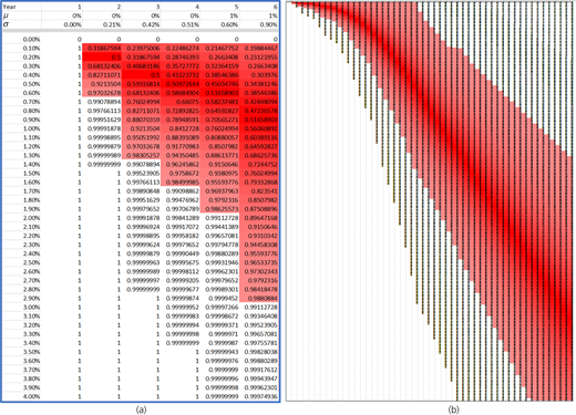
The number of additional users due to growth in population is modelled over time based on the expectation of the demographic dynamics. The development of the population since 1990 in the three larger municipalities in close proximity to the new highway section – that is, Uster, Wetzikon and Hinwil – has been significant. Despite the fact that population growth in these municipalities is only one of the factors influencing the traffic on the highway among others (e.g. level of employment) – that is, more travel generated by the people travelling from Winterthur to Oerlikon over the highway than travel generated by the people living in these municipalities – the population of these municipalities was considered a good proxy for the number of users of the highway for two reasons: (a) it represents a significant portion of the traffic and (b) the dynamics of this population are similar to those of the wider region. At the moment, Uster has approximately 35 000 inhabitants in comparison with 1990 with about 27 000 (Kanton Zürich, 2020). The trend line for Uster indicates that the population will increase linearly by 370 people every year. With the same assumption for the cities of Wetzikon and Hinwil, which currently have 25 000 and 11 000 inhabitants, respectively (Kanton Zürich, 2020), their expected population increase is 320 and 110 inhabitants per year, respectively. At the moment, there are approximately 54 000 cars per day on the existing part of the highway A15 (GIS-Browser, 2020). About one-half of the vehicles are currently between Uster, Wetzikon and Hinwil (Kantonsrat Zürich, 2020). Based on this information, it was estimated that an additional 800 inhabitants in the area (i.e. 370 Uster + 320 Wetzikon + 110 Hinwil) will lead to an increase in daily traffic volume of 456 cars. With these assumptions, the daily car traffic is expected to increase by 730 users per year, as the average occupancy rate is 1.6 persons per car (BFS, 2015). Since these projections are based on projections of the future population, they are not certain. The uncertainty associated with the projections is modelled by using a normal distribution with the projected values as the mean value and a standard deviation of 5% initially and rising to 15% in 50 years (Figure 2). This was assumed to represent adequately the progressively decreasing degree of confidence in the projections over time.
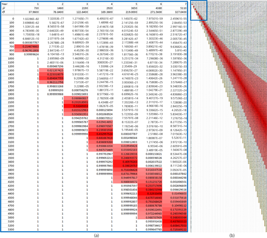
Model of the uncertainty with respect to the number of additional users due to growth in population (NPopulation), with a zoom on the probability distribution (a) for the first 7 years and over (b) the 50-year period. On the X-axis are the years from 1 to 50 and on the Y-axis the possible additional or less users of the highway. The red colour marks the area between 0.5 and 99.5% probability. The stronger the red colour, the higher the probability
Model of the uncertainty with respect to the number of additional users due to growth in population (NPopulation), with a zoom on the probability distribution (a) for the first 7 years and over (b) the 50-year period. On the X-axis are the years from 1 to 50 and on the Y-axis the possible additional or less users of the highway. The red colour marks the area between 0.5 and 99.5% probability. The stronger the red colour, the higher the probability
Number of additional users due to the growth in the use of private vehicles over trains
The number of additional users due to the growth in the use of private vehicles over trains (NTrain) is modelled over time as function of the changes in the modal split between private vehicles (i.e. cars and trucks) and public means of transport (i.e. trains), which is seen as rather uncertain, depending on a number of factors. On one side, the percentage of persons travelling in private vehicles may increase, and the percentage travelling by rail may decrease, due to the potential future developments in the auto industry (i.e. autonomous and electric vehicles). This phenomenon might even be exacerbated by an intrinsic characteristic of autonomous-vehicle-based mobility: the need for empty trips to pick up passengers. For example, a recent publication (Meyer et al., 2016) underlined that this new mobility paradigm could bring up to 1.5 empty trips per person and day, which would mean a 50% increase in traffic. On the other side, there may be a decrease in the number of persons travelling in private vehicles and an increase in the number of these travelling by rail. The factors that support this trend include (a) the extension of the railway service between Uster and Rapperswil, which runs parallel to the new highway section, and (b) the possibility that widespread use of autonomous vehicles might result in an increase in users sharing autonomous vehicles, which could lead to a 60% reduction in traffic (Zhang et al., 2015).
In this work, the uncertainty associated with these trends was modelled as a normal distribution by assuming that over the next 50 years, the number of persons travelling in individual motorised vehicles instead of travelling by rail can go from a max increase of 13 000 to a max decrease of 100 with the mean tendency of increasing of 4300 and a probability over the extreme normally distributed. The increasing lack of confidence in the predictions over time is captured by increasing the standard deviation over time, from a nearly inexistent deviation in the first year – that is, it is very unlikely that any modal split change will happen in the first year – to 50% in the last year – that is, the technological evolution required to enable shift in the modal split balance could evolve in a large set of paths over the next 50 years (Figure 3).
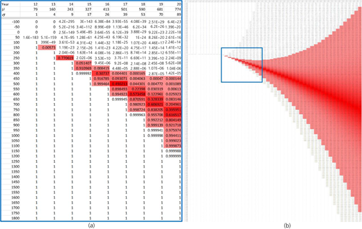
Model of the uncertainty associated with the number of additional users due to the growth in the use of car over trains (NTrain) with a zoom on the probability distribution (a) for the years 12–20 and (b) over the 50-year period
Model of the uncertainty associated with the number of additional users due to the growth in the use of car over trains (NTrain) with a zoom on the probability distribution (a) for the years 12–20 and (b) over the 50-year period
Reduction in the number of users due to the growth of the home-office working mode
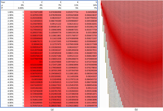
The reduction in the number users due to the growth of the home-office working mode (NHomework,t) is modelled considering the increasing interest in, and acceptance of, being able to work from home (‘Teleheimarbeit’ 2020). As the Covid-19 crisis has shown, it is possible and, in some cases, even advantageous to work from home – for example, by reducing commuting time (source: Martani et al., 2022). It is assumed in this example that the mean percentage of the time people work from home is likely to increase by 0.07% per year (Figure 4). Due to the large uncertainty associated with the prediction, however, a normal distribution is assumed with a standard deviation starting at 10% – that is, in the current pandemic situation, there is already a significant degree of uncertainty associated with the number of people who will be working from home a year from now – and increases to 50% of the mean value after 50 years – that is, this uncertainty is even larger in the future due to the multiple future paths that this trend could take, depending on evolution of videoconferencing technology and the degree of acceptance of distributed work in the long term.
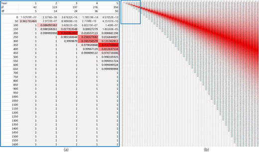
Model of the uncertainty in the share of home-office mode (DH0), with a zoom on the probability distribution (a) for the first 5 years and (b) over the 50-year period
Model of the uncertainty in the share of home-office mode (DH0), with a zoom on the probability distribution (a) for the first 5 years and (b) over the 50-year period
Percentage of autonomous vehicles
The percentage of autonomous vehicles that will be circulating on the road in the years of the analysis period is rather uncertain. In previous work, this has been simplified to depend on three time-consecutive events, each of which is subject to substantial uncertainty (Elvarsson et al., 2021): (a) vehicles must first be ready for deployment – that is, full vehicle autonomy, by technology reaching level 5 (according to the SAE standard on the levels of driving automation (source: Shuttleworth, 2019); (b) vehicles must be legally allowed to enter circulation on current roads; and (c) people must be willing to select travelling by automated vehicle instead of by human-driven vehicle. On highways, it is presumed that level 4 will be sufficient. For this work, it is assumed that the technology for fully autonomous driving on highways could be ready for deployment between 2025 and 2035 (Becker et al., 2016; Litman, 2017). The likelihood of the second and third events is much more difficult to predict. Using recent work on these topics (Altenburg et al., 2018; Elvarsson et al., 2021), the uncertainty of the technological evolution and commercial widespread of autonomous vehicles was modelled over the 50-year time period as a normal distribution (Figure 5). The mean starts at 0.1%, which expresses the belief that it is almost impossible that an autonomous vehicle would be ready to circulate in the immediate future, and ends at 79%, which represents the market expectation by 2050 (Bösch et al., 2018; Litman, 2017). The standard deviation is assumed to start at 0% – that is, at the moment, neither the technological nor the legal conditions to enable autonomous driving level 5 are in place and it is almost certain that this will also be the case 1 year from now – and increases to 22% of the mean value after 50 years – that is, this variable could take multiple paths in the future due to technological, legal and commercial reasons – that is, according to a recent survey, current drivers seem to retain a certain degree of scepticism in using autonomous vehicles, although the technology is ready for use (Etzioni et al., 2020).
Model of the uncertainty associated with the percentage of autonomous vehicles (DAV), with a zoom on the probability distribution (a) for the first 5 years (left) and (b) over the 50-year period
Model of the uncertainty associated with the percentage of autonomous vehicles (DAV), with a zoom on the probability distribution (a) for the first 5 years (left) and (b) over the 50-year period
Percentage of electric vehicles
Electric vehicles are a well-established technology (Li et al., 2019) and have a promising commercial prospective in Switzerland. According to Mobilitätsmonitor 2018, 72% of those interviewed in the country consider buying an electric vehicle in the future (Bieri et al., 2018). However, the future commercial success of electric vehicles depends on numerous factors, such as (a) the development of long-lasting and fast-charging batteries, (b) the cost of electricity in Switzerland as it denuclearises by 2050 and (c) the widespread use of less carbon dioxide intense ways to produce electricity (Schärer, 2018). Based on the work by Schärer (2018), the uncertainty associated with the percentage of electric vehicles, DEV, was modelled as shown in Figure 6 – that is, as a normal distribution with constantly rising mean and standard deviation. The mean starts at 2%, which is a prudential representation of the current market share of electric vehicles in the country (BFS, 2019), ending at 57%, which represents the market expectation by 2050 (Ajanovic, 2015). The increasing standard deviation captures the difficulty of narrowing the trajectory of this variable. The standard deviation is assumed to start at 0% and increase to 27% of the mean value after 50 years, meaning that the uncertainty in the amount of electric vehicles in 1 year from now will be rather certainly approximated to that of this year, but in 50 years, it could follow any of a wide range of trajectories. It is to be noticed that the percentage of electric vehicles is here assumed to be the same for automated and human-driven vehicles.
Model of the uncertainty associated with the percentage of electric engine vehicles (DEV), with a zoom on the probability distribution (a) for the first 5 years and (b) over the 50-year period
Model of the uncertainty associated with the percentage of electric engine vehicles (DEV), with a zoom on the probability distribution (a) for the first 5 years and (b) over the 50-year period
Designs and future modifications
In this section, a number of alternative designs are presented for the completion of the A15 highway, along with the possible interventions to adapt the infrastructure in the future, when possible – that is, for the design in which the option to trigger future adaptations is created.
Designs
The five investigated designs, with their main characteristics and estimated construction costs, are shown in Table 6. They range from not building the extension at all (i.e. doing nothing) to the myopic design for accommodating the current needs proposed in the master plan by Canton Zürich (i.e. the traditional design) to a highly robust design, oriented to accommodate all envisioned potential future needs (i.e. with different degrees of robustness both the separate-lanes design and the maximum design), to a flexible solution that is designed both to accommodate the current needs and to be easily convertible – that is, with the potential to be modified easily, in case that the need changes (i.e. the flexible design). Each design is explained in detail in the following sections.
Overview of the five designs for the highway extension
| Design | Illustration | Construction cost: billions CHFa | |
|---|---|---|---|
| Do nothing | — | 0 | |
| Traditional design | Road | Tunnel | 1.1 |
 |  | ||
| Bridge | Ramp | ||
 |  | ||
| Separate-lanes design | Road | Tunnel | 1.2 |
 |  | ||
| Bridge | Ramp | ||
 |  | ||
| Flexible design | Road | Tunnel | 1.5 |
 |  | ||
| Bridge | Ramp | ||
 |  | ||
| Maximum design | Road | Tunnel | 1.65 |
 |  | ||
| Bridge | Ramp | ||
 |  | ||
The cost of construction does not include the costs of land acquisition, as it is considered that the infrastructure owner already owns enough land to accommodate any design
1 CHF = US$1.07
DO NOTHING
The do-nothing solution implies that no highway extension is built, resulting in zero cost of construction but potentially causing substantial costs for users and the indirectly affected public over the next 50 years if the traffic demand rises, which, due to the absence of the highway connection, will trigger an increase in accidents, travel time and carbon dioxide emission.
TRADITIONAL DESIGN
The traditional design is the one defined from the master plan of the canton and includes the construction of the new highway extension with two lanes in each direction, for the use of both human-driven vehicles and autonomous vehicles (mixed traffic). This design includes separate lines in both tunnels and bridges for each driving direction, while the on and off ramps of the highway are built on the ground. The costs for the traditional design have been estimated by the canton of Zurich to account for approximately 1.1 billion CHF 1 CHF = US$1.07 (Kantonsrat Zürich, 2020).
SEPARATE-LANES DESIGN
The separate-lanes design is conceived with road, tunnels and bridges with two separate lanes per driving direction, one for human-driven vehicles and one for autonomous vehicles. In light of the criticality of a mixed-driving mode in terms of accidents in the road access – that is, when human-driven vehicles and autonomous vehicles share the same ramps, the number of accidents is likely to rise substantially due to difficulties for autonomous vehicles to react to sudden human movements (Maurer et al., 2015) – the on and off ramps are separated for human-driven vehicles and one for autonomous vehicles. This design is expected to cost 1.2 billion CHF, which is 0.1 billion CHF more than cost of the traditional design (Eberle, 2020). The cost has been estimated assuming that the bridges at the on and off ramps cost 10 million CHF each, which results in 80 million CHF. The remaining 20 million CHF is the estimated cost for the separation of the lanes – that is, building traffic barriers and separated signalling.
FLEXIBLE DESIGN
The flexible design, as is the traditional design, contains two lanes in each direction, for the use of both human-driven vehicles and autonomous vehicles (mixed traffic). In the case of the flexible design, though, the bridges are designed with a load-bearing capacity that enables extension to a third lane per direction, and the tunnels are excavated from the beginning with the width required to accommodate a third lane per direction. Additionally, the on and off ramps are designed as bridges to allow a third lane to pass underneath. The cost of the flexible design is estimated to be 1.5 billion CHF in light of the difference with the works for the construction of the highway with the traditional design. An open highway was assumed to cost 500 CHF/m2 and the tunnel 8000 CHF/m2 (Anon, 2005) (adjusted according to an average annual inflation of 0.8% (source: Macrotrends, 2022)). A bridge was assumed to cost 2600 CHF/m2 (Tiefbauamt Kanton Zürich, 2019). The (two lines) tunnels, which are 11 m wide and 4.5 km long, were estimated to cost an additional 400 million CHF. The on and off ramps are estimated to cost approximately 100 million CHF for this design. The value has been estimated considering that the additional load-bearing capacity required to allow adding a third lane (i.e. a 50% increase in the weight) in the future without any structural reinforcement implies an extra cost in concrete and reinforcements of approximately 25% of the costs – that is, 20 additional million CHF to the 80 million CHF estimated for the ramps in the separate-lanes design.
MAXIMUM DESIGN
The most robust design considered is the maximum design, which is conceived with three lanes from the beginning (two human-driven vehicle lanes and one autonomous vehicle lane). It is assumed that this variant is 5% less expensive than the flexible design after future interventions are triggered, because everything can be done in one step, saving on the second set-up cost for the working place. This has resulted in an estimated cost of 1.65 billion CHF.
Future modifications and triggering logic
For this example, the assumption is made that no future modifications will be made to the designs that have not been predisposed to modifications through flexibility. Therefore, the only design in which the option to trigger future adaptations is created is the flexible design. Specifically, three interventions are conceived to adapt the highway, when needed. The interventions are summarised in Table 7, along with the pertinent triggering logic. A detailed explanation of the interventions is then discussed in the following sections.
Overview of the three possible interventions for adapting the flexible design
| Intervention | Illustration | Cost:a millions CHF | Triggering logic | |
|---|---|---|---|---|
| Convert the highway into two separate traffic lanes per direction | Road | Tunnel | 50 | Number of autonomous vehicles > number of human-driven vehicles |
 |  | |||
| Bridge | Ramp | |||
 |  | |||
| Convert the highway into three separate traffic lanes per direction | Road | Tunnel | 200 | >10 000 users/h |
 |  | |||
| Bridge | Ramp | |||
 |  | |||
| Add a charging station |  | 5 | Number of electric vehicles > number of combustion vehicles | |
Cost derived from the estimate in the newspaper article by Anon (2005)
CONVERTING THE HIGHWAY INTO TWO SEPARATE TRAFFIC LANES PER DIRECTION
The highway is converted into two separate traffic lanes. This includes adapting the road, tunnels and bridge to two separate traffic lanes and adding separate on and off bridge ramps for the independent access of autonomous vehicles. This intervention will be triggered when there are more autonomous vehicles in the system than human-driven vehicles. This is because it is assumed that when, in a given simulation, there are more autonomous vehicles than human-driven vehicles on the road, the benefits are expected to exceed the costs after just 5 years – that is, the benefit associated with the expected reduction in the number of accidents due to mixed use of the road is higher than the costs of lane separation (i.e. 50 million CHF).
CONVERTING THE HIGHWAY INTO THREE SEPARATE TRAFFIC LANES PER DIRECTION
The highway is converted into three separate traffic lanes. This includes expanding the width of the road, tunnels and bridges to create an additional lane per direction and connect it to both the bridges and ground on and off ramps. I2 is triggered when the number of human-driven vehicles is higher than 10 000 per hour. This is because 10 000 users/h is considered the maximum acceptable amount of traffic for operating a single line road (Werdin et al., 2004) – that is, the probability of traffic congestion and accidents are still likely to be below predefined thresholds.
ADDING A CHARGING STATION
The highway can be modified to include a charging station per direction. I3 is triggered when the number of electric vehicles is higher than the number of vehicles with combustion engines. The rationale for this intervention is that the investment on a plugging station along the highway is considered justifiable only when electric engines become mainstream.
Simulation
In this step, the Monte Carlo method is used – based on the uncertainty modelled on the key variables – to estimate the total expected costs for each design over 50 years. This way the objective function introduced in the section headed ‘Boundaries, interventions and the objective of the evaluation’ is used to estimate dynamically the total cost for each design – that is, considering the simulated future trend of all the variables, in each simulation. The operation is repeated – that is, the variables are simulated until the results stabilise, which, in the context of this work, occurs with 1000 simulations. This resulted in 1000 estimated cost profiles for all four designs. In the next section, the results are compared to identify the best design (i.e. the one that is trusted to ensure the lowest costs).
Before discussing the results, it is interesting to observe the effect that the simulated variables have had on the four directly affected uncertain parameters (Figure 7) (as from Table 4) – that is, the number of autonomous vehicles (N AV, t), human-driven vehicles (N NV, t), electric engines (N EV, t) and combustion engines (N CV, t). In Figure 7, top, it is shown that, in terms of simulated driving mode, the number of users of human-driven vehicles (Figure 7(a)) rises up to year 15, with a peak of 59 891 users/day on average. This is mainly due to the increase in the simulated total number of cars. After that, it decreases until year 50, when there are, on average, still 20 310 users of human-driven vehicles per day, following the modelled use of autonomous vehicles. On the other hand, the simulated users of autonomous vehicles (Figure 7(b)) increase after a start-up period of about 10–15 years. At the end of the 50-year period, the expected number of daily users is 69 806. In terms of propellant mode (Figure 7, bottom), the simulated users of combustion engine vehicles (Figure 7(c)) decrease in the first 29 years from an initial average of 54 781 users/day to 34 296 users/day and then remains roughly constant for another 20 years. In the end, it is estimated to increase again to 40 274 users/day on average, because the growth of road users is greater than the growth of electric motor users. Meanwhile, the simulated users of electric engine vehicles (Figure 7(d)) increase more in the first years than in the following ones, with the curve increasingly flattening to 49 842 users/day in the 50th year. This is mainly due to the modelling of the use of electric vehicles.
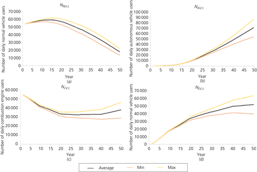
Effect of the simulated variables on the numbers of (a) human-driven vehicles (N NV, t), (b) autonomous vehicles (N AV, t), (c) combustion engines (N CV, t) and electric engines (N EV, t)
Effect of the simulated variables on the numbers of (a) human-driven vehicles (N NV, t), (b) autonomous vehicles (N AV, t), (c) combustion engines (N CV, t) and electric engines (N EV, t)
Results
In Table 8, an overview is presented of the results of the simulations, in terms of the median and standard deviation of the expected total costs.
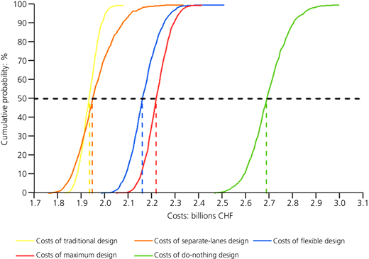
As from Table 8, the traditional design has the lowest estimated cost – that is, 1934 million CHF – closely followed by the separate-lanes design with nearly 1947 million CHF (i.e. between the two designs, there is only a 13 million CHF difference). Following, in descending order of costs, are the flexible design with roughly 2160 million CHF and the maximum design with approximately 2220 million CHF. It is noticeable that the expected cost of the worst design is significantly higher – that is, 14.8% more than that of the low-cost designs. The significance of the median expected cost of all designs is also supported by the relatively small standard deviations, which are around 2–4% of the costs, with the highest standard deviation for the do-nothing and separate-lanes designs (i.e. approximately 83 million CHF) and the smallest deviation for the traditional design (i.e. approximately 40 million CHF).
Median and standard deviation of the costs of the different designs
| Median: millions CHF | Deviation from the cheapest design: % | Standard deviation: millions CHF | |
|---|---|---|---|
| Do nothing | 2693 | +39.2 | 83 |
| Traditional design | 1934 | 0 | 40 |
| Maximum design | 2220 | +14.8 | 54 |
| Separate-lanes design | 1947 | +0.7 | 83 |
| Flexible design | 2160 | +11.7 | 63 |
Both the median and the standard deviation of the costs of all designs are shown in Figure 8 in the form of cumulative probability distributions. The figure shows that the flexible, maximum and do-nothing designs do not overlap in any area. This means that these designs are not cheaper than the others in any percentage range. In contrast, the curves of the separate-lanes design and the traditional design do cross at around 30% cumulative probability, indicating that there is a greater uncertainty associated with the cost estimate of the separate-lanes design than that of the traditional design. Indeed, since the separate-lanes design has a flatter curve and therefore a larger standard deviation, this design is less expensive than the traditional design in approximately 30% of cases – that is, in all simulations in which the demand for autonomous vehicles picks up substantially in the early stage of the investigated period.
Despite the fact that the traditional design is the optimal one when considering the intervention costs and all measures of service together (Figure 8), it worth noticing that, when only the measures of service (i.e. the travel costs – including both accident costs and costs of lost travel time – and or environmental costs) are isolated, the order of preference of the designs changes significantly. In Figure 9, it is shown how the travel costs with the do-nothing design are by far the largest – that is, with a median of around 2.6 billion CHF. The travel costs with all the other designs are relatively close, with the lowest cost (0.82 billion CHF) associated with the maximum design and the flexible design the second lowest (0.87 billion CHF). This is due to the fact, despite their cost of implementation, these designs guarantee better accommodation of the various possible needs of future traffic (i.e. increasing, stagnant or decreasing traffic of vehicles with different propellant and driving modes) than the do-nothing design. In about 18% of all simulations, the travel costs with the separate-lanes design are higher than those of the traditional design, due to the predominant increase in the number of vehicles with either one of the two traffic modes – for example, in the simulation in which the number of autonomous vehicles grows significantly more than that of human-driven ones, the separation in line is counterproductive, leading to a lack of space for the autonomous vehicles and excess of space for the human-driven ones.
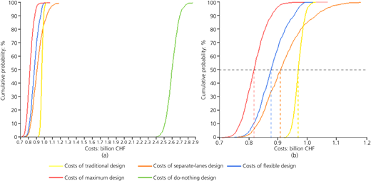
(a) Cumulative probability of the travel costs from 1000 simulations for all designs; (b) zoom on the traditional, maximum, separate-lanes and flexible designs (right)
(a) Cumulative probability of the travel costs from 1000 simulations for all designs; (b) zoom on the traditional, maximum, separate-lanes and flexible designs (right)
Finally, when looking closely at the triggering frequencies of the three possible interventions (Table 9), for the case in which the highway is constructed with the flexible design, the following can be noticed over 1000 simulations.
The intervention to modify the highway into two separate traffic lanes per direction is triggered nearly always (i.e. 95% of the cases). This is due to the fact that the number of autonomous vehicles will quite certainly overcome the human-driven ones over the course of the next 50 years, in light of the uncertainty modelled.
The intervention to modify the highway into three separate traffic lanes per direction is triggered only 11.6% of the time. This is due to the fact that the overall traffic is rather unlikely to exceed 10 000 users/h over the course of the next 50 years, in light of the uncertainty modelled.
The intervention to add a charging station is triggered 62.6% of the time, which is due to the fact that the probability that the number of electric vehicles is relatively likely to overcome that of the combustion ones over the course of the next 50 years in light of the uncertainty modelled.
Trigger states and the number of appearances in 1000 simulations
| Intervention | Triggering logic | Number of appearances in 1000 simulations |
|---|---|---|
| Convert the highway into two separate traffic lanes per direction | Number of autonomous vehicles > number of human-driven vehicles | 951 |
| Convert the highway into three separate traffic lanes per direction | >10 000 users/h | 116 |
| Add a charging station | Number of electric vehicles > number of combustion vehicles | 626 |
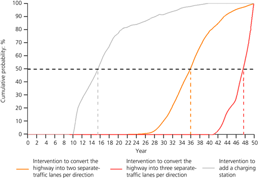
Besides the triggering frequency, the triggering time of each intervention is interesting. In Figure 10, it can be seen that the interventions to add a charging station is triggered most frequently at a very early stage (with the highest probability to occur in year 16). This is because in the simulations where the electric vehicles exceed 50% of the total vehicles on the road, this tends to happen relatively soon, given the current matureness of the electric vehicle technology. Meanwhile, intervention I1 tends to be triggered more often at a later stage (with the highest probability to occur in year 36). The reason is that, even in the simulations with a rising number of vehicles on the A15, it takes time for traffic to exceed 10 000 users/h. The tendency towards late triggering is even stronger for intervention I2 (which has the highest probability to occur in year 48), because for the autonomous vehicles to exceed 50% of the vehicles on the road, both the technological and legal conditions have to be created, which is not likely to happen in the near future.
Discussion
This work shows the potential of using a quantitative method for the evaluation of alternative highway designs, considering the uncertainty of future mobility patterns in terms of both traffic intensity and traffic mode (i.e. driving mode and propellant mode). Specifically, in the example of the A15 highway, the quantification of future costs and benefits considering the uncertainty associated with the future mobility patterns and management flexibility has provided significant advantages in determining the optimal design, compared with the traditional road design evaluation. This is particularly the case with reference to the following aspects.
Formulating the objective mathematically to define how the service provided by the highway is to be quantified. This is done accounting explicitly for the service required by each of the involved stakeholders and enables optimising designs with respect to a set of defined goals.
Modelling the uncertainty probabilistically on all key external parameters affecting the objective function. The variables affecting the objective function are identified and modelled. This is done probabilistically considering the range of plausible variability around the foreseeable most probable scenario for each parameter and allows the modeller to make use of the best current knowledge on future uncertain variables for running insightful simulations.
Developing alternative possible designs, including flexible ones. This consists of developing designs that have different potential to minimise the negative effects of the uncertainty on the variables modelled to be compared – that is, myopic designs, robust designs and flexible designs (with the pertinent future changes) – and triggering logic.
Simulating future scenarios considering the uncertainty associated with the key variables, which allows the estimation of the costs and benefits for all designs. This increases the ability to evaluate accurately the net benefit of each design, avoiding the mistake of approximating all the variables to their expected value in a unique, most likely wrong, scenario.
Notwithstanding the aforementioned merits, the use of the evaluation method also has limitations, which are principally related to the need to do the following:
Modelling the uncertainty: The determination of the ranges of the key variables and their probabilities of occurrence is a delicate step that requires trusting the opinions of experts – for example, the uncertainty on the future evolution of traffic demand cannot be modelled projecting the past trends into the future, as the factors that have led to the past trends are not constant. The effects of external factors are hard to predict, and this is conducted through expert evaluation.
Determining the triggering logic: The definition of the triggering conditions – that is, the conditions under which it is decided that to modify the highway – opened with a flexible design – is used, is inherently uncertain and has to be defined in a way that captures what is most likely to happen. If this is not true and the changes are not triggered as they are defined in the model, the outcome of the estimate will not reflect reality.
Determining the time of execution of interventions: The time required to plan and execute any change on a highway often involves public debates and, in certain cases, even a public vote, which can cause significant delays or even blocking of the works, which are difficult to account for (Brinkman and Lin, 2019). This can be even more the case in the future with the development of citizen design practice for new highways (Mueller et al., 2018).
Despite these limitations, the evaluation method can help infrastructure planners identify the most valuable design and intervention strategies, by increasing the ability of decision makers to estimate accurately the net benefit associated with each design in light of the uncertainty modelled on the future traffic demand.
Conclusion
In this work, the potential of using a real-option-based evaluation method to obtain an indication of the best designs for new highways was shown, considering the uncertainty on the future mobility patterns and infrastructure flexibility. The evaluation method was shown using a fictive but realistic case study based on the extension of the A15 highway in Switzerland, by defining a panel of alternative designs, including flexible ones; modelling the uncertainty on the future traffic demand; and simulating future scenarios to identify the optimal design – that is, the one with the highest expected net benefit according to the scenarios simulated.
The results of the example indicate that considering the costs of intervention on the infrastructure, as well as the impact on travel and on the environment, the best design consists of a regular highway with two mixed lanes per direction (traditional design). This means that the traditional design is the one that optimally results in the lowest cumulative intervention, travel time accident and environmental costs. However, when the impact on the travel time and safety is isolated, the analysis shows that the flexible design has an advantage compared with the more myopic ones. In both cases, the simulations indicate that the worst decision would be to not build the highway extension at all, as the future traffic demand largely justifies the investment to build the highway extension. Although this analysis confirms the opportunity to choose a traditional design in this case, the analysis has provided this conclusion by systematically evaluating the alternative designs, based on the effect that the uncertain future mobility patterns has on a variety of stakeholders, instead of taking the risk to neglect these.
Despite the encouraging results of this preliminary work, the authors acknowledge that the use of this methodology requires significantly more effort to model the many factors affecting the transport system – for instance, the rate of shared trips. In terms of further steps, it would be of prominent interest to develop the work in two main directions.
Improve the way that uncertain future mobility is modelled to affect the service, considering the complexity of the real world – for example, using a systems dynamics model to illustrate the consequences on travel time and accidents that future uncertainties may have.
Integrate considerations on the effect of possible variations in the spatial development of the region – that is, consider which area might be developed first – for example, Hinwil or Wetzikon – and how the foreseen development will affect the service in detail – for example, how much additional traffic they will trigger over time.
Further study the types of modifications that enable the ease and timeliness of modifying infrastructure and the evolution of the contextual factors influencing the demand – for example, the post-pandemic trend with the home-office working mode.
Integrate considerations on the network dynamics and network capacity to refine the estimated effect of the infrastructure decision on traffic.
It would also be of interest to develop the simulations further by modelling the mutual dependencies of the variables and conduct a sensitivity analysis to investigate the effect of the triggering logic and the discount rate on the results. Besides the limitations of this exploratory work, the paper clearly demonstrates the possibility of its use to improve highway design, considering future uncertainty.
Acknowledgement
The authors wish to acknowledge the help of Arnór Elvarsson from the Infrastructure Management Group at ETH Zürich, for his help in reviewing the work.
