Freight forwarders as value creators in maritime logistics: a system dynamics approach Open Access

Freight forwarders stand out as one of the most crucial transport and logistics service providers by serving as essential intermediaries between shippers and carriers. Initially focused on basic forwarding services, the role of freight forwarders has gradually expanded to intermodal transport and a growing inclination towards outsourcing logistics operations (Sohail and Al-Abdali, 2005). Nowadays, they are entrusted with a comprehensive array of global transportation and logistics services, including warehousing, inventory control, packaging and the real-time tracking of shipments. By offering these indispensable transport and logistics solutions, freight forwarders play an ever more critical role in moving raw materials and finished products for the shippers.

Due to the multifaceted role freight forwarders play in the provision of logistic services, they are inevitably confronted with intricate operational challenges (Vaidyanathan, 2005). Their responsibilities entail adeptly coordinating a diverse array of logistic activities to meet the broad and varied demands of their clientele (Liu and Lyons, 2011). This is further compounded by the dynamic nature of the freight forwarding industry and the perpetual evolution of technology, which necessitates their capacity to anticipate and effectively address diverse requirements (Lee and Song, 2018). In the domain of maritime transport and logistics systems, the operational intricacies faced by freight forwarders (hereby referred to as forwarders for better readability) are heightened due to the indispensable need for seamless interaction with other key stakeholders, such as port terminal operators and shipping lines (Panayides and Song, 2013). Any disruptions in this integration could result in escalated costs and service delays, thereby emphasizing the paramount importance of efficient collaboration with other involved parties. Addressing these challenges requires an integrated approach to operational planning and decision-making to mitigate the cascading effects of isolated decisions.

This study adopts a value chain perspective to analyze and refine the complexities of freight forwarding operations. By offering a structured framework, the value chain approach highlights the key activities that drive the competitive advantage and value creation (Porter, 1985). It emphasizes two critical dimensions: value creation (Jaakkola and Hakanen, 2013) and value measurement (Daaboul et al., 2014). In this context, identifying and prioritizing value-creating activities forms the foundational analysis, while revenue generation serves as a proxy for value realization. Decomposing freight forwarding operations into specific activities facilitates the systematic identification of influencing factors and their interdependencies, ultimately enabling the development of targeted strategies to optimize value creation. Considering the complicated nature of the interplay processes in the value creation of forwarders, a detailed and holistic analytical approach is required. This study employs system dynamics (SD) to empirically investigate value-creating activities within maritime logistics. SD enables a comprehensive analysis of complex system structures and operations, offering an effective method for measuring value creation within the chosen transport and logistics sector (Barlas, 1996; Sterman, 2000).

The study investigates freight forwarders at Tanjung Priok Port, Indonesia, recognizing the country’s strategic reliance on maritime transport as one of the world’s largest archipelagic nations. Tanjung Priok handles approximately 60% of Indonesia’s total container traffic (World Shipping Council, 2021), making it a critical node in national logistics. Freight forwarders operating here manage significantly higher cargo volumes, contributing substantially to economic development, yet face persistent challenges, including container delivery delays, limited alternative ports for import-export activities, and a shortage of nearby warehousing facilities (Indonesian Trucking Association, 2021; Kearney, 2022). A deeper understanding of value creation in this context can inform strategic initiatives by both the government and industry stakeholders to address these challenges and strengthen their competitive advantages.

In this context, the study aims to empirically investigate the mechanisms of value creation among freight forwarders, using Tanjung Priok as a case study. It contributes to both the conceptualization and practical application of the value chain framework. Although prior research has adapted the value chain concept across various contexts (Prajogo et al., 2008; Bosch-Mauchand et al., 2012), notable gaps remain, particularly the tendency to examine value-creating activities in isolation, overlooking their interdependencies (Fyrberg Yngfalk, 2013). Addressing this gap, the study adopts a system perspective by applying SD to explore the interactions among factors influencing value creation. It also advances the literature by offering a detailed exploration of freight forwarders’ value creation mechanisms, extending prior macro-level analyses (Lam and Zhang, 2014; Lee and Song, 2010; Vural et al., 2019). Furthermore, this research introduces quantitative methods for value measurement, moving beyond the qualitative focus of earlier studies. In addition to enriching the academic discourse, this research equips forwarders and policymakers with meaningful perspectives to identify and prioritize strategic areas for improvement, thereby enhancing value creation in the freight forwarding sector.

The remainder of this paper is organized as follows: Section 2 presents freight forwarding value creation in maritime logistics. Section 3 examines the employment of SD as a method for investigating the value creation in freight forwarding. Section 4 articulates the research findings and provides a detailed discussion. Section 5 addresses both policy and managerial implications arising from the study. The paper ends up with the concluding remarks in Section 6.

Value chain perspectives have been introduced by Porter (1985) to offer a framework for understanding how companies generate value at the firm level. This model provides an in-depth look at the series of activities through which activities add value by converting raw materials into finished goods for delivery to end-users. Consequently, the value chain approach is characterized by two main aspects: value creation and value measurement. Value creation involves identifying customer needs and transforming them into value-adding activities. Value measurement, on the other hand, aims to assess the benefits that forwarders receive from fulfilling customer needs.

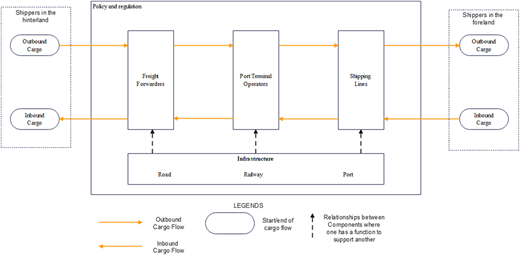
Forwarders emerge as critical logistic facilitators for the seamless execution of international trade operations on behalf of shippers. Their primary function initially was to forge connections between cargo owners and shipping lines (Saeed, 2013). However, with the escalating trend towards logistic outsourcing, the scope of their roles has considerably evolved within the supply chain network (Barber, 2008). Forwarders currently extend a myriad of global logistic services that encompass inventory management, inland transportation, warehousing, packing and tracking. Figure 1 illustrates a visual representation of forwarders’ integral positioning within the context of maritime logistic systems, which are delineated as a set of interrelated components designed to facilitate the movement of goods through ocean carriage. Complementing forwarders, port terminal operators manage cargo handling operations and shipping lines are charged with the transportation of cargo across ports.

Facing multifarious operational challenges in the process of providing logistics services, forwarders are required to adeptly manage an extensive array of logistics functions to meet the wide-ranging and evolving needs of their clientele (Liu and Lyons, 2011). These challenges are further intensified by the dynamic nature of the freight forwarding industry and ongoing technological advancements, demanding their capacity for foresight and adaptable response to a spectrum of demands (Lee and Song, 2018). In maritime logistics systems, the complexity of forwarders’ tasks is amplified by the essential requirement for seamless collaboration with pivotal entities, such as port terminal operators and shipping lines (Panayides and Song, 2013). A lack of integration in this collaborative effort can precipitate costs and delays in service. The unpredictable outcomes stemming from the complexities inherent in the freight forwarding industry can be mitigated by holistic understanding, which is essential to circumvent counterintuitive behaviors that may hinder the development of effective policy interventions. This study embraces a value chain perspective as a means to decipher the intricacies of freight forwarding, scrutinizing the interconnected logistics activities undertaken by forwarders that are essential to value creation.

In general, the value generated by any service provider can be approached from two distinct perspectives: customers and service providers. From the customer’s standpoint, value is seen as the advantages customers accrue from engaging with forwarders, during and after the service (Ulaga and Chacour, 2001; Vargo and Lusch, 2004). In contrast, from the service provider’s perspective, the concept of value measurement is tied to the benefits gained by forwarders after fulfilling their customer’s requirements (Daaboul et al., 2014).

This study adopts the service provider’s perspective to understand the activities through which forwarders create value as it allows for a more objective assessment of value compared to evaluations from the customer’s perspective (Randall et al., 2014). Customers may not completely grasp the full extent of benefits they receive, leading to potentially subjective evaluations that may not accurately capture the comprehensive value delivered by service providers (Lambert and Burduroglu, 2000; Daaboul et al., 2014). Therefore, analyzing value from the service provider’s standpoint yields important insights into how forwarders successfully fulfill customer requirements.

Adopting the perspective of service providers for understanding the notion of value, this research identifies revenue as a metric for value measurement, aligning with the concept proposed by Porter (1985). Revenue represents the total amount of money earned through the provision of services to their clients. This indicator corresponds to how value is measured from the service providers’ viewpoint, where revenue is recognized as the benefits gained by forwarders after providing services to their customers.

From a theoretical standpoint, two prominent concepts of value creation by service providers: the service-dominant (S-D) Logic and the goods-dominant (G-D) Logic. S-D Logic posits that value is determined by the customer and is created continuously along the customer journey, from initial engagement with the service or product to its eventual utilization (Vargo and Lusch, 2008). In this framework, the relationship between the producer and the customer is symbiotic, where both the players work together to create value and co-value for each other (Vargo and Lusch, 2008; Gummesson and Mele, 2010). Conversely, G-D Logic suggests that the service provider is the one who creates and defines value, which is subsequently transferred to the customer (Ulaga and Chacour, 2001; Vargo and Lusch, 2008). This approach delineates a clear distinction between the roles of the producer, who is responsible for creating and imparting values, and the customer, who consumes the value (Vargo and Lusch, 2004, 2008).

While both S-D Logic and G-D Logic offer distinct viewpoints on value creation, they converge on the principle that a sequence of activities plays a crucial role in the process of creating value. This study opted for the G-D Logic to analyze value creation in freight forwarding based on two primary considerations. First, forwarders tend to focus on refining their own operations instead of participating in collaborative endeavors with their customers to co-create value. Second, G-D Logic provides the ability to precisely measure value, facilitated by the well-defined roles of producers and customers, which demarcate clear boundaries. This foundational concept guides this research in understanding and empirically examining value creation in freight forwarding as it helps to understand the distinct value created by the freight forwarders.

Exploring the mechanisms through which forwarders create value unveils the diverse roles they play. Numerous studies have delved into the vast spectrum of logistical services offered by freight forwarding companies. For instance, Vaidyanathan (2005) conceptualizes a framework that disaggregates the operations of forwarders into four principal categories: transportation, warehousing, inventory and logistics management and customer service. Complementing this framework, Lee and Song (2018) delineate a range of value-adding activities, including freight forwarding services, inventory management, packing, warehousing and inland transportation. Collective insights from these studies shed light on the multifaceted role of forwarders that extends substantially beyond the transportation of cargo for shippers. This research identifies inland transportation and warehousing management as the most critical logistics activities forwarders perform, making substantial contributions to their value creation (Kayakutlu and Buyukozkan, 2011). By enhancing these key activities, forwarders stand to enhance their value generation and strengthen their competitive position in the market.

Inland transportation is the primary value-adding activity of forwarders, as it enables the movement of cargo between shippers and destination points via ports (and vice versa). This activity is crucial for connecting the sea and landside since the customers are often located in diverse and far-flung hinterland areas that are difficult to access without efficient transportation services. Shippers, as the primary customers of forwarders, demand efficient transportation services to ensure the timely delivery of their goods and minimize transportation costs (Sohail and Sohal, 2003; Sohail and Al-Abdali, 2005). To meet customer requirements and based on the principles of G-D Logic, inland transportation could create value when the transfer of goods to and from the port is conducted seamlessly. Such condition results in a higher volume of goods being transported to the port, thereby enhancing the benefits accrued by forwarders. The primary determinant of the smooth movement of goods via inland transport is port access. Enhanced access to the port allows forwarders to reduce delivery times, increase the frequency of their transport operations, and ultimately augment the volume of goods transported. Lean et al. (2014) assert that enhancing inland transport infrastructure is instrumental in supporting better port access, which in turn positively influences regional economic development. Moreover, the proximity of shippers to ports plays a pivotal role in the value creation process, as this factor determines the ease of port access for forwarders. Yudhistira and Sofiyandi (2018) highlight that closer proximity of shippers facilitates easier delivery of goods, thereby increasing trade activities and fostering economic development. Consequently, to maximize the value created by inland transportation, forwarders must strategically manage delivery distances through meticulous planning and routing vehicles effectively (Kayakutlu and Buyukozkan, 2011).

The second value-adding activity of forwarders is providing warehousing management services, which involves storing shippers’ cargo until it can be physically distributed to its intended destinations. Warehousing management is essential for keeping cargo in good condition prior to delivery (Frazelle, 2002; Waters, 2003). From the perspective of forwarders, this value-adding activity creates significant value when they can maximize cargo storage, which enhances the benefits they receive. Achieving this condition requires sufficient warehouse capacity to ensure ample space for goods without causing overcrowding (Kayakutlu and Buyukozkan, 2011). This approach not only adds value for forwarders but also stimulates regional development, as the establishment of warehouses facilitates the movement of goods throughout the production chain (Barros Simões et al., 2024). Furthermore, effective warehousing management entails streamlined processes within warehouses (Bowersox et al., 2002). Such efforts reduce storage time and permit a higher volume of freight to be handled within the same timeframe.

Value creation and measurement have been studied using various discrete event simulations (Daaboul et al., 2014) and network value analysis (Peppard and Rylander, 2006), which at times fail to fully interpret the dynamics of value creation within systems. In this regard, SD provides a better understanding of the value creation of the activities by the actions within a system as highlighted by Barlas (1996) and Sterman (2000). In the context of freight forwarding, SD conceptualizes forwarders as a system encompassing two primary value-adding activities, which are interconnected and collaboratively contribute to value creation. The SD approach allows for a comprehensive examination of policy implications in both the short and long term (Besiou et al., 2014; Raoofi et al., 2024). Hence, it will be instrumental in formulating strategies that bolster the value generation in freight forwarding.

In general, SD employs the crucial concepts of stock and flow derived from control system theory (Sterman, 2000; Sweeney and Sterman, 2000). These concepts help to understand how systems change over time, with stock referring to any variable that accumulates or depletes and flow representing the rate at which the stock changes. Mathematically, the quantity of stock is determined by subtracting the rate of the outflow variable from the rate of the inflow variable, starting from an initial stock value. The status of a stock at a time $(t)$ is represented by the integral of the net flow, which is the inflow $(s)$ minus the outflow $(s)$⁠, calculated from the initial time (⁠$to$⁠) to the present time as represented in the following equation:

SD perceives a system as an intricate assembly of multiple stocks and flows, interconnected through their interactions, potentially creating feedback loops. Such a loop occurs when alterations in a stock influence the flows in or out of that stock (Ford, 2019). The idea of feedback loops is crucial as it illustrates how actions can produce unforeseen effects and highlights the complex interplay among the components of the systems.

As this study applies this general framework of SD for measuring the value creation of various logistics activities of freight forwarders, this section outlines a systematic and operationalizable approach for measuring value creation for freight forwarders using SD. The interrelationships among key variables are systematically derived and grounded in a synthesis of peer-reviewed literature spanning logistics, freight forwarding and SD. These variables and their interdependencies are then visually represented through the development of a causal loop diagram (CLD), which elucidates the dynamic feedback mechanisms inherent to value creation processes.

Following the development of CLDs that qualitatively explain how value is generated through each activity, the next phase involves converting these CLDs into stock flow diagrams (SFDs). These SFDs mathematically define relationships between variables. At this stage, the variables identified in the CLDs are meticulously categorized into four distinct classifications: stocks, flows, formulas and constants. The equations that define stocks, flows and formulas are derived from a comprehensive analysis of relevant academic literature in the fields of logistics, freight forwarding and SD. Simultaneously, the data for constants is gathered from statistical reports, such as government databases and directly from the forwarders.

As SD provides the value using situation, after getting the results from SFDs, the study employs two ways of validating the results: (1) structural validation and (2) behavioral validation, which are the most common ways of validation approaches in SD studies (Barlas, 1996). The structural validation emphasizes that the model’s structure accurately reflects the actual systems under examination, while the behavioral validation ensures that the model’s behavior is consistent with the actual observable behavior of the systems. If the model fails to meet the behavior validation standards, it would require to reiterate the CLDs and SFD processes until achieving satisfactory results.

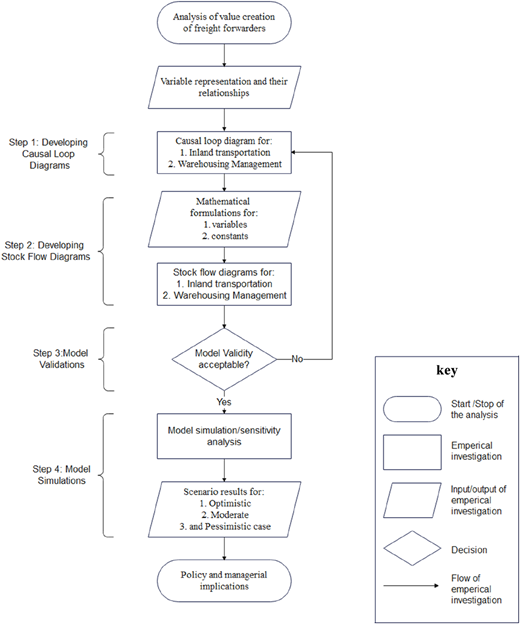
Once the model attains an acceptable outcome, it can then be utilized to perform simulations, allowing for an evaluation of how enhancements in value creation processes influence the overall value created by forwarders. The study develops three scenario analyses (i.e. optimistic, moderate and pessimistic) for the value of cargo and how to adjust the controllable variables to maximize the value creation of the freight forwarding industry in the region. An in-depth understanding of what to do under different scenarios has both policy and managerial implications. Figure 2 illustrates a flowchart that outlines the steps involved in the empirical investigation of value creation within the freight forwarding sector.

For the empirical application, the study focuses on freight forwarding activities in the region of Tanjung Priok port in Jakarta, Indonesia, as a case study. Indonesia is an archipelagic nation with a heavy dependence on maritime transport. The Tanjung Priok port plays a crucial role in Indonesian maritime logistics systems as it handles around 60% of the nation’s container traffic movement (World Shipping Council, 2021). Within the context of Indonesia, forwarders’ value creation is demonstrated through the inbound and outbound logistics flows. The outbound flow encompasses the transportation of goods from shippers in the hinterlands to the port, whereas the inbound flow covers the movement of goods from the port to shippers located in the hinterlands.

The CLDs and SFDs for individual value-adding activity for the freight forwarders are developed, after which they are combined for the entire freight forwarding sector to observe the overall value creation.

Within maritime logistics systems, inland transportation serves as the critical link between hinterland shippers and ports. At Tanjung Priok Port, forwarders predominantly rely on trucking to connect Jakarta’s industrial zones with the port. This reliance stems from insufficient railway infrastructure, a limitation noted in studies such as Kaddoura et al. (2024), which highlighted similar challenges in Switzerland. The value generated by inland transportation, reflected in revenue, is primarily influenced by the volume of freight transported to and from the port.

Building on Porter’s (1985) framework, this analysis employs revenue as a key metric to evaluate the value-added contribution of forwarders through inland transportation services. The aggregate revenue of forwarders in Indonesia is used to measure their economic contribution at the national level. As highlighted by Aschauer et al. (2015), factors influencing this revenue include freight volume, delivery distance and freight rates. An increase in any of these elements enhances revenue and consequently the economic value generated by forwarders.

Freight volume is closely tied to delivery time, as detailed in studies by Aschauer et al. (2015), Poles (2013), Saeed (2013) and Vlachos et al. (2007). Poles (2013) emphasized that reducing delivery time can significantly increase the volume of transported cargo. Delivery time is influenced by factors such as transport distance and vehicle speed, which interact in complex ways. For instance, Liu et al. (2021) observed that longer distances generally extend transportation times, while increased truck speeds reduce them (Aschauer et al., 2015). Road capacity also plays a crucial role, with enhanced infrastructure allowing faster freight movement. However, higher traffic volumes can lead to congestion, slowing down trucks and creating a cyclical effect where increased freight volumes further exacerbate road congestion (Liu et al., 2021; Naumov et al., 2020).

Freight rates in inland transportation are determined by market dynamics. When demand decreases relative to supply, rates drop and vice versa. The demand for inland transportation services is primarily driven by the volume of freight needed for transport, as noted by Aschauer et al. (2015) and Sachan et al. (2005). Increased demand typically raises freight rates as forwarders adjust prices in response to market conditions (Sterman, 2000). However, higher freight rates may reduce service usage as shippers explore alternative options (Sterman, 2000). On the supply side, increasing trucking capacity lowers freight rates by boosting service availability, benefiting shippers with reduced costs.

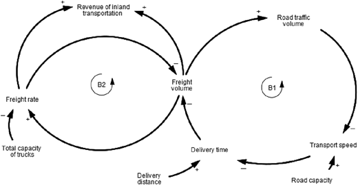
Figure 3 illustrates the variables influencing inland transportation services and their interrelationships. Two feedback loops (B1 and B2) are identified. In loop B1, an increase in transported freight volume raises road traffic, reducing transport speed and lengthening delivery times, ultimately lowering forwarders’ capacity to handle additional freight. Loop B2 captures the relationship between freight volume and rates; rising volumes increase rates, which then curtail demand, leading to a subsequent decrease in transported volume.

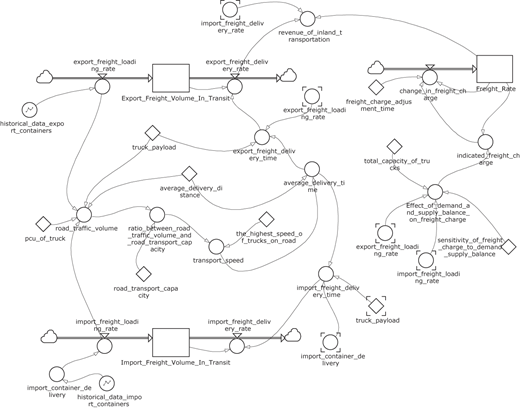
The CLD is translated into a SFD in Figure 4, enabling the representation of these dynamics through quantitative mathematical relationships. Key stock variables include export freight volume in transit, import freight volume in transit and freight rate. These stocks represent quantities that accumulate over time, reflecting the system’s state at any given moment. Export and import freight volumes increase with loading rates and decrease upon delivery. Freight rate, another critical stock variable, reflects the costs of inland transportation and significantly influences revenue.

Auxiliary variables such as revenue, road traffic volume, transport speed and delivery time are represented through equations to streamline calculations and provide a clear depiction of value creation. Constants, including delivery distance and road capacity, are held fixed due to data limitations and their typically stable nature in the short term. The inland transportation value creation process begins when forwarders transport freight between ports and hinterland shippers. Export freight volume (⁠$EFV(t))$ in transit serves as the stock at any time t, denoted as presented in Equation (1), can be estimated as follows:

where $EDC(t)$ represents export freight volume received from shippers and $EDr(t)$ the delivered volume at time t. Similarly, import freight volume in transit, $IFV(t)$⁠, is expressed as

Here, $IDC(t)$ and $IDr(t)$ denote the import freight volume received from ports and delivered to hinterland shippers, respectively. Historical data from the Tanjung Priok Port informs these calculations.

Road traffic volume $VRD(t)$ depends on truck payload $L$⁠, average transport distance $AD$ and a weightage factor for truck traffic $PCU$⁠:

Transport speed $sRD(t)$ varies with traffic volume and maximum road capacity $CRD$​, constrained by the free-flow speed $SRD$​:

where $λ,ω$ and μ are the parameters that relates with the specification of roads.

Delivery time ^[1], influenced by transport speed, affects freight delivery rates, which in turn drive revenue. Freight rate ^[2] $FRIT(t)$ dynamics are modeled using Sterman’s (2000) hill-climbing method, capturing adjustments in response to demand-supply imbalances. Revenue $RIT$⁠, representing inland transportation’s value, is calculated as

The study excludes delivery distance’s potential impact on revenue due to the Indonesian pricing structure, where freight rates depend solely on volume. Additionally, limitations in data availability preclude modeling the inverse relationship between freight rates and volume. Through CLD and SFD analysis, the research provides a comprehensive view of inland transportation’s role in value creation within Indonesia’s maritime logistics system.

Warehousing management focuses on maintaining cargo in optimal condition until its physical delivery to end customers. Shippers, as cargo proprietors, may opt to store their goods temporarily in forwarders’ warehouses instead of sending them directly to ports or hinterland destinations. As highlighted by Frazelle (2002) and Waters (2003), warehousing management involves overseeing warehouse inventory, which encompasses the total freight volume stored in forwarders’ facilities. The value created for forwarders through this activity is closely tied to the volume of stored freight.

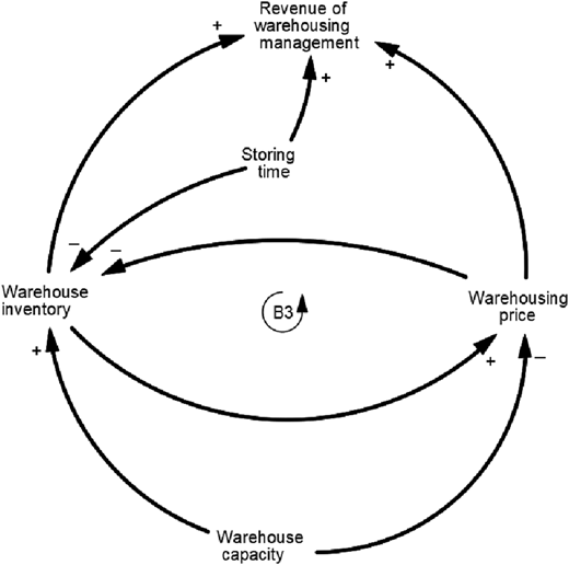
Figure 5 illustrates the process by which forwarders generate value through warehousing management, as depicted in a CLD. This diagram identifies key variables and their interrelations, emphasizing a single balancing loop (B3). In this loop, an increase in warehouse inventory drives up warehousing prices, which subsequently reduces the volume of freight stored.

Warehousing management serves to ensure cargo remains in good condition before delivery to end customers. Frazelle (2002) and Waters (2003) describe this process as encompassing the oversight of warehouse inventory. Meanwhile, Rathore et al. (2021), along with Sterman (2000), argue that factors such as warehousing price and storage duration positively influence revenue generated through warehousing management, reflecting the value created by forwarders in offering these services.

The interplay between warehousing service charges and inventory levels is significant. Sterman (2000) observes that increased warehouse inventory, often a result of higher demand for storage, typically leads to higher warehousing prices. However, elevated costs can prompt shippers to explore alternative storage solutions, potentially decreasing the demand for forwarders’ services. On the supply side, Sterman (2000) explains that increased warehouse capacity may lead to a surplus in warehousing services, driving prices down – a scenario beneficial to shippers, who enjoy lower costs.

Rathore et al. (2021) and Sterman (2000) identify two key factors affecting forwarders’ inventory management capabilities: warehouse capacity and storage time. Warehouse capacity, defined as the maximum inventory volume a warehouse can accommodate, influences freight volumes and the overall market dynamics of warehousing services. Increasing capacity not only supports higher freight volumes but also enhances the supply of services, potentially lowering prices (Sterman, 2000). Storage time, the speed at which inventory moves from warehouses to customers, is another critical factor. Reducing storage time allows for more efficient operations, enabling faster inventory turnover and optimizing warehouse utilization (Rathore et al., 2021; Sterman, 2000). Warehouse inventory emerges as a critical stock variable within the SFD of warehousing management. It serves as an essential indicator of how effectively forwarders store shippers’ goods and create value. This dynamic variable accumulates through incoming inventory and depletes as goods are dispatched.

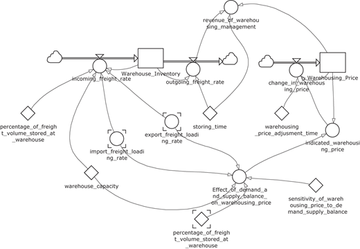
Following the development of the CLD, the next step involves constructing an SFD model. This process begins with categorizing CLD variables into stocks, flows and auxiliary variables. In the SFD for warehousing management, two key stock variables are identified: warehouse inventory and warehousing prices. Figure 6 visually represents these components, highlighting their role in value creation.

Warehouse inventory is selected as a stock variable because of its capacity to reflect operational performance and value addition. It accumulates via incoming inventory rates and diminishes as goods are dispatched. Warehousing price, the second stock variable, captures the dynamic fluctuations in service costs, directly influencing revenue. Both variables are vital in understanding the value generated through warehousing services. Flow variables impacting these stock variables are elaborated upon later.

Auxiliary variables, such as warehousing revenue, simplify the computation of derived value and clarify the value-creation process. Storage time is treated as constant due to data constraints, while warehouse capacity is considered fixed because of its infrequent adjustments.

The value derived by forwarders through warehousing hinges on the optimal inventory stored in their facilities. The total inventory volume at time t, $WI(t)$⁠, can be mathematically defined as follows:

where $Wi(t)$ represents the incoming freight rate and $Wo(t)$ represents the outgoing freight rate at time t (Poles, 2013; Sterman, 2000).

In Indonesia, shippers often utilize forwarders’ warehouses for temporary storage instead of immediate shipment to final destinations. Consequently, the ratio of freight volume transported to warehouses $υW$, and the import/export freight loading rate influences incoming freight volume. Warehouse capacity (⁠$CW$⁠) also determines the maximum cargo that can be stored:

Outgoing freight flow considers the average storage duration (⁠$Ts$​):

Warehousing prices (⁠$WP(t)$⁠) are modeled using a hill-climbing method, adjusting dynamically to demand-supply imbalances (Sterman, 2000). Prices change according to:

with $PW(t)$ as the rate of price adjustment:

The indicated price $iw(t)$ depends on demand-supply effects:

where $Ew(t)$ is the balance effect, influenced by warehouse capacity $(Cw$​) and demand levels (⁠$Dr(t)$⁠):

Finally, the value created through warehousing management, $RWM$⁠, is expressed as:

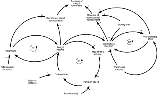
Due to the lack of data availability, the study does not incorporate the typically negative relationship between warehousing price and warehouse inventory. The total value creation of the freight forwarders is the aggregation of the revenue from inland transportation and warehousing management. Figure 7 provides a detailed depiction of the entire value creation process, which illustrates the interrelationships among variables. This figure highlights two key concepts of value creation as discussed in Section 2: first, the adoption of the service providers’ perspective on value measurement, where revenue is used as a proxy for value; and second, the application of G-D Logic, which asserts that value creation occurs exclusively within the internal operations of forwarders.

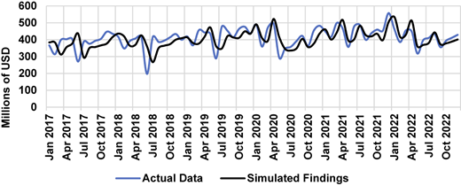
The simulated total value creation of the freight forwarders using the SD model approach is validated against the actual data. Following the guidelines established by Barlas (1996) and Sterman (2000), structure validity assesses how well the SD model reflects the actual structure of the systems being analyzed, while behavior validity evaluates the model’s ability to accurately replicate the behavior patterns observed in real-world systems.

Figure 8 illustrates the model’s capacity to predict behavior patterns with reasonable accuracy by comparing simulated outcomes against actual data on the value created by forwarders. Sterman (2000) outlines several statistical methods for evaluating the behavioral validity of SD models. Various statistical tools are utilized, including the Mean Absolute Percentage Error (MAPE), bias proportion (⁠$UM$⁠), variance proportion $(US$⁠) and covariance proportion (⁠$UC$⁠), as well as Theil’s Inequality Coefficient (TIC). These metrics are employed to compare the simulated behavior of the model with the actual system behavior and to identify potential sources of error within the model.

Table 1 provides an error analysis of the SD model concerning value creation by forwarders, where the selected variable is compared to the corresponding values observed in real systems from 2017 to 2022. The evaluation of the proposed SD model, based on the total value generated by forwarders, demonstrates its notable predictive accuracy, as indicated by the satisfactory MAPE and TIC values for the variable. Furthermore, an analysis of inequality statistics for this variable emphasizes issues related to unequal covariance and unsystematic errors. This analysis suggests that, despite some variations at individual data points, the model effectively captures the overall trends of the actual system. This finding is consistent with the recommendations of Sterman (2000), which highlights the model’s ability to reflect real-world systems’ behaviors.

A scenario analysis was conducted to evaluate the sensitivity of logistic operations in freight forwarding to their value creation potential. By simulating diverse operational conditions, the analysis elucidates how strategic modifications to specific activities can optimize value generation for freight forwarders, as conceptualized within service-dominant logic (Vargo and Lusch, 2004, 2008). The investigation focuses on two logistics activities – inland transportation and warehouse management – assessing their individual contributions to value maximization. Subsequently, an integrated framework is proposed to examine the synergistic effects of concurrent enhancements across all value-adding activities on overall value creation.

The analysis evaluates improvements in value creation by systematically adjusting variables within the operational system. To align with real-world constraints, variables are categorized as either exogenous (uncontrollable external factors, such as import/export container volumes) or endogenous (controllable internal factors, including stock levels, workflow efficiency and auxiliary parameters). While endogenous variables remain fixed in the model, exogenous variables are manipulated to reflect varying degrees of operational influence.

Three scenario archetypes – pessimistic, moderate and optimistic – are formulated to quantify the potential outcomes of value-adding interventions. These scenarios establish a spectrum of projections to inform strategic decision-making:

1. Pessimistic scenario: Assumes subhistorical growth rates, with export and import container volumes increasing at 2 and 1.5% annually, respectively.

2. Moderate scenario: Aligns with historical trends, projecting 3.5% growth for export containers and 2.5% for import containers.

3. Optimistic scenario: Anticipates growth exceeding historical averages, with export and import containers expanding at 5 and 3.5%, respectively.

Each scenario incorporates detailed adjustments to endogenous variables specific to individual value-adding activities, enabling a granular assessment of operational trade-offs and opportunities. By contextualizing these outcomes, the framework equips decision-makers with actionable insights to prioritize resource allocation and strategic initiatives under uncertainty.

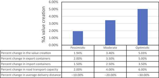
Inland transportation entails moving containers between ports and shippers in the hinterlands. At Tanjung Priok port, these containers are predominantly transported to and from the Karawang Industrial area, situated approximately 70 kilometers away. To improve this value-adding activity and assess its impact on the overall value creation of forwarders, the study modifies two controllable variables in the SD model: road transport capacity and average delivery distance. Road transport capacity refers to the maximum number of trucks that a particular road can handle under normal conditions. A constant growth of road length of about 4% as reported by Statistics Indonesia (2024) is considered a proxy for projecting increases in road transport capacity. Consequently, for the simulations, a 4% increase in road transport capacity for the moderate scenario is utilized, adjusting this figure to 6% in the optimistic scenario and 2% in the pessimistic scenario. For moderate and pessimistic scenarios, the average delivery distance is expected to decrease by 20 and 10%, respectively. Considering the projected growth of export and import containers, the scenarios for improving inland transportation are detailed in Table 2.

Figure 9 illustrates the impact of improvements in inland transportation on the overall value of forwarders, specifically through enhancing road transport capacity and reducing average delivery distance. The figure shows that a pessimistic scenario results in a value increase of 1.94%, while the moderate and optimistic scenarios enhance the value to 3.46 and 5.03%, respectively. It reveals that enhancing transport capacity, shortening delivery distances and increasing export and import container volumes all contribute positively to the value of forwarders. Therefore, to shift from a pessimistic to an optimistic scenario to generate greater value creation, it is crucial to substantially increase road transport capacity while simultaneously shortening the average delivery distance.

Enhanced transportation infrastructure directly increases the value of inland transportation services for freight forwarders in Indonesia. Specifically, upgrading road capacity and reducing delivery distances enable forwarders to operate more efficiently. This relationship is illustrated through a SD model, which reveals how forwarders generate value via inland transportation in maritime logistics. Improved road capacity allows faster transport speeds and shorter delivery distances, further reducing transit times. Together, these factors enable forwarders to make more frequent trips between ports and hinterlands customers, increasing the volume of containers transported. Higher container volumes, in turn, amplify the economic value created by forwarders.

Existing logistic operations at Tanjung Priok Port face significant delays. According to the Indonesian Trucking Association (2021), traffic congestion is a major barrier. For instance, transporting containers between industrial zones like Karawang and the port can take 12 h during peak congestion – nearly triple the 4.5-h duration under normal conditions. This congestion stems from road networks operating beyond capacity during peak hours and the lack of direct toll road access between the port and industrial areas. Simulations confirm that expanding road capacity would alleviate delays, allowing forwarders to deliver more containers faster and thereby generate greater value.

A further challenge is the absence of alternative ports near Jakarta that are capable of handling export-import containers. To address this, the Indonesian government is developing the Patimban Port, located 145 kilometers from Tanjung Priok. Once operational, Patimban will serve industrial regions currently underserved due to their distance from Tanjung Priok. By providing an additional logistic hub, this port is expected to shorten delivery routes, reduce transit times and enhance forwarders’ operational flexibility. These projections align with simulation results, highlighting the importance of minimizing delivery distances in inland transportation.

While existing literature often emphasizes port access as a driver of regional economic growth, freight forwarders also benefit directly from improved infrastructure. For example, Lean et al. (2014) found that better inland transport networks boost economic activity by simplifying good movement to and from ports. Such improvements allow forwarders to handle larger cargo volumes, increasing their profitability. This aligns with studies showing that proximity to hinterland markets strengthens forwarders’ competitive advantages, underscoring the interdependence between infrastructure quality and logistics efficiency.

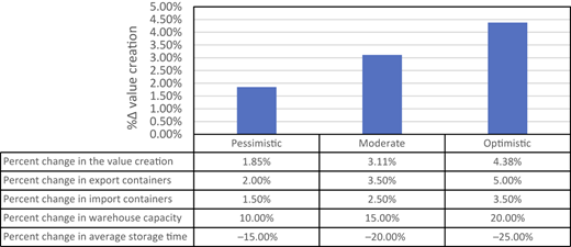
Within the context of Tanjung Priok port, Indonesian forwarders handle inbound cargo by storing it upon arrival from the port and subsequently delivering it to shippers in the hinterlands. Conversely, they manage outbound cargo by storing it after collection from shippers in the hinterlands, prior to delivering it to the port. Two variables representing warehousing management improvements are modified: warehouse capacity and average storing time. Warehouse capacity, which refers to the total capacity of forwarders’ warehouses, grew by 15% from 2022 to 2023 in Jakarta and Western Java (SDI, 2024). Thus, the study assumes a moderate scenario with a 15% increase in warehouse capacity, modifying this to 10 and 20% for pessimistic and optimistic scenarios, respectively.

Specifically, in the optimistic scenario, the average storage time is reduced by 25%. This reduction means a decrease in one week from the current average storage time of four weeks. A 20% reduction is also considered for the moderate scenario and a 15% reduction for the pessimistic scenario. Alongside the projected growth of export and import containers, Table 3 outlines the detailed assumptions for pessimistic, moderate and optimistic scenarios to improve warehousing management.

The overall impact of these enhancements on the value creation of forwarders is illustrated in Figure 10. Under the pessimistic scenario, strategic enhancement in warehousing management results in a value growth of 1.85%. Meanwhile, the moderate and optimistic scenarios show even greater growth, reaching 3.11 and 4.38%, respectively. Across all scenarios, increasing warehouse capacity and reducing average storage time, along with the rise in export and import containers, contribute positively to the value of forwarders. Additionally, transitioning from the pessimistic to the optimistic scenario requires significant efforts to simultaneously provide higher warehouse capacity and shorter storage time, both of which are crucial for achieving higher value growth.

Improvements in warehousing activities can boost the value generated by Indonesian freight forwarders. Expanding warehouse capacities and reducing storage durations enable forwarders to handle larger cargo volumes while accelerating freight turnover. Increased capacity allows more goods to be stored, while shorter storage times improve operational efficiency, enabling higher throughput within the same timeframe. Together, these enhancements amplify the economic value derived from warehousing services.

A critical shortage of warehouses near Tanjung Priok Port exacerbates logistical pressures (Kearney, 2022). Rising demand—driven by the growth of the Fast-Moving Consumer Goods (FMCG) sector, imported goods, e-commerce, and the digital economy—has outpaced existing infrastructure. To address this gap, expanding warehouse capacities near the port is imperative. Simulations in this study corroborate this need, demonstrating that increased capacity consistently improves forwarders’ value creation across all scenarios. Additionally, shippers increasingly prioritize reduced storage times to lower costs. However, many Indonesian warehouses lack advanced IT systems and rely on manual processes, leading to inefficiencies and prolonged storage periods. Addressing these bottlenecks through modernization and process optimization is essential to increase throughput and competitiveness.

These findings align with established literature on warehouse management. For instance, Kayakutlu and Buyukozkan (2011) highlight that adequate warehouse space prevents overcrowding and ensures smoother logistics operations, directly supporting forwarders’ ability to manage larger inventories. Similarly, Bowersox et al. (2002) emphasize the role of streamlined processes in effective warehousing. Reducing storage times–a proxy for operational efficiency–further validates how optimized workflows enhance value creation. By integrating these principles, Indonesian forwarders can strengthen their logistical capabilities and align with global best practices.

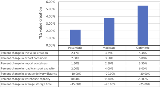
Figure 11 illustrates how individual controllable variables can affect the overall value creation using the scenario analysis. Under a pessimistic scenario, combined improvements increase the value by 2.17%, while moderate and optimistic scenarios yield higher gains of 3.79 and 5.48%, respectively. Targeting specific activities alone – such as inland transportation (5.03% value increase) or warehousing (4.38%) in the optimistic scenario – delivers significant benefits. However, integrating enhancements across all activities produces marginally greater value (5.48%). This suggests that focusing solely on individual infrastructure (e.g. roads or warehouses) may result in diminishing returns without a holistic strategy.

The modest added benefit of combined improvements can be explained by balancing feedback mechanisms inherent in freight forwarding systems. These mechanisms, which stabilize growth, may offset gains when too many changes occur simultaneously (Vaidyanathan, 2005). For instance, expanding road capacity and warehouse space might strain other interconnected processes, such as labor availability or port handling, reducing overall efficiency. This aligns with research highlighting the complexity of logistics systems, where changes in one area can trigger unpredictable ripple effects (Besiou et al., 2014). Thus, while integrated strategies hold promise, their success depends on managing interdependencies to avoid counterproductive outcomes.

Indonesia’s national logistic policy, the Indonesian Logistics Systems (ILS) outlined in Presidential Directive Number 26/2012, focuses on strengthening the forwarding sector through infrastructure development. However, this policy lacks specific guidance regarding the type and scale of infrastructure improvements needed at the regional level. While general road infrastructure enhancements can improve operational efficiency (Arbués and Baños, 2016), they may not optimize the potential of specific regional contexts. Critically, the ILS overlooks persistent congestion, particularly at port access points, which significantly impedes efficient logistics operations.

This study, focusing on Indonesia’s largest port, Tanjung Priok, underscores the need for a reassessment and potential redesign of maritime logistics policies in developing the road transport infrastructure. Enhancing road infrastructure in Jakarta, particularly access to Tanjung Priok port, is crucial for facilitating efficient container movement. Improved port access enables faster inland transport services for forwarders, boosting import and export activities and contributing to economic development. This aligns with research demonstrating the positive impact of improved road infrastructure on regional economic growth (Lean et al., 2014). The urgency of this improvement is further highlighted by Statistics Indonesia (2024), which reports Jakarta’s current road ratio at 7.3% of the city area, significantly below the ideal 12%. Therefore, continued road infrastructure development is essential to maximize the contribution of maritime logistics systems to Jakarta’s economic growth.

Beyond road infrastructure, developing new warehouse facilities near the Tanjung Priok port is a critical priority for the Indonesian government and forwarders. This initiative is essential to meet the growing warehousing demand driven by the expanding manufacturing and e-commerce sectors. Increased warehouse capacity empowers forwarders to handle larger freight volumes, enhancing their value creation potential.

This study also has managerial implications for Indonesian forwarders operating within the Tanjung Priok port. In the context of inland transportation, given the critical importance of delivery distance to the port in the value creation processes (Kayakutlu and Buyukozkan, 2011), forwarders could consider implementing shipment consolidation strategies by collaborating closely with shipping lines and shippers. By segmenting shipments from multiple shippers into a single truck, forwarders can design routes that minimize travel distance and delivery time. This approach represents a more feasible solution for forwarders, given the considerable challenges and extensive resources required for shippers to relocate their factories closer to the Tanjung Priok port.

Moreover, Indonesian forwarders should enhance the efficiency of warehousing management services by streamlining the processes within warehouses to reduce average storage time. This effort is crucial in reducing the freight storage time in warehouses, thereby increasing the overall freight volume that can be stored (Bowersox et al., 2002). An effective approach to improving warehouse efficiency is to adopt a digital solution that could help forwarders manage and oversee daily warehouse operations, from the arrival of freight into the warehouse to its departure. Given that most warehouses in Indonesia are still managed manually, this initiative represents a significant shift toward digitalization.

Indonesian forwarders need a holistic strategy to maximize value creation. However, they must be aware of potential unintended consequences. Continuous monitoring and evaluation are crucial for identifying and adjusting strategies as needed to ensure their effectiveness. Forwarders should prioritize inland transportation improvements over warehouse management, as this activity has a greater impact on overall value creation. Each component, particularly value-adding activities, contributes uniquely to overall system performance.

Given that freight forwarders operate within maritime logistics systems involving port terminal operators and shipping lines, improvements in inland transportation and warehouse management by freight forwarders can facilitate smoother operations at terminals and better scheduling for shipping lines. These enhancements by one actor can, in turn, generate a positive impact across the broader logistic network, highlighting the interconnected nature of the system. However, realizing these benefits requires more than isolated improvements – it demands a collaborative and integrated approach across the logistics chain. Seamless coordination among actors is crucial, not only to minimize operational disruptions but also to drive value creation throughout the entire system. For instance, initiatives that foster cross-stakeholder collaboration – such as the implementation of shared digital platforms or synchronized planning mechanisms – are increasingly necessary to improve overall outcomes in maritime logistics.

This study contributes to both conceptual and applied domains by advancing the scholarly discourse on value creation within maritime logistics systems. It proposes a structured SD framework to analyze the intricate logistic activities of freight forwarders, addressing gaps in existing qualitative methodologies. The empirical design introduced here establishes a foundation for (1) evaluating value generation in freight forwarding sectors across diverse regional contexts and (2) extending investigations to other maritime stakeholders, such as port terminal operators and shipping lines, to better understand sector-wide interdependencies.

From a practical perspective, the research provides actionable insights for policymakers and managers aiming to optimize value creation. Through scenario analysis – optimistic, moderate, and pessimistic trajectories – the study demonstrates that prioritizing inland transportation improvements yields the most significant value gains. Concurrent enhancements in warehousing management may further amplify these benefits. However, given the nonlinear dynamics inherent to freight forwarding operations, the findings underscore the necessity of continuous strategy evaluation and adaptive risk management to mitigate unintended consequences.

Nevertheless, this study acknowledges limitations. Its focus on Tanjung Priok Port (Jakarta, Indonesia) as a single case study constrains the generalizability of findings due to location-specific geographic and operational factors. Future research could expand empirical analyses to multiple regions and develop SD models to explore value-creation mechanisms among other maritime actors. Such efforts would elucidate systemic interactions and contextual variability, fostering a more holistic understanding of maritime logistic ecosystems.

The authors would like to express their sincere appreciation to the editor and the two anonymous reviewers for their crucial and constructive comments during the revision and resubmission process, which have significantly enhanced the clarity and readability of the article.

The supplementary material for this article can be found online.