


Despite evidence that infants affect families’ economic and social behaviors, little is known about how young children influence their parents’ political engagement. I show that U.S. women with an infant during an election year are 3.5 percentage points less likely to vote than women without children; men with an infant are 2.2 percentage points less likely to vote. Suggesting that this effect may be causal, I find no significant decreases in turnout the year before parents have an infant. Using a triple-difference approach, I then show that universal vote-by-mail systems mitigate the negative association between infants and mothers’ turnout.
Introduction
Voting helps form the basis for strong and accountable democracies. Turnout from individuals with diverse policy preferences can ensure that politicians are responsive to the needs of a representative set of their constituents (Lijphart, 1997), and high turnout has been linked to policy outcomes that favor working-class voters such as increases in pensions (Fowler, 2013). Despite the importance to policy outcomes, U.S. turnout levels have averaged only 40–60% in national elections over the past half century. While research in political science and economics has documented a host of factors that affect turnout levels, including individual education and age, election competitiveness, weather, and the overall economic situation (e.g., Blais, 2006; Charles and Stephens, 2013; Geys, 2006; Leighley and Nagler, 2013; Powell, 1986; Wolfinger and Rosenstone, 1980), there has been limited exploration into the impact of having young children on U.S. voter turnout.1 This is especially striking considering that the birth of a child is a highly disruptive event shown to affect work habits, ease of travel, and health and may therefore increase the physical/logistical barriers to going to the polls (Albrecht et al., 2018; O’hara and Swain, 1996). Furthermore, since families with young children may have different policy preferences than others, their exclusion from the political process may lead to lower support from the government and thus long-term consequences on children’s well-being (Hoynes et al., 2016). This paper documents the relationship between having a young child and turnout in the United States. It also explores whether state systems that reduce physical/logistical costs of voting such as universal vote-by-mail affect this relationship.
The key difficulty in estimating the relationship between young children and voter turnout is that having a child is not an exogenous event. It is associated with a range of characteristics including age, financial stability, and unmeasurable characteristics such as community orientation that may themselves drive voting behavior. To address this concern, I first include a large number of individual and state-level controls to account for measurable characteristics that may affect voting behavior. Second, I confirm the absence of a turnout effect for parents who will have an infant in the next year, exploiting variation in the exact year of birth. This mitigates concerns about differences in unmeasurable characteristics between parents and non-parents.
Using data from the Current Population Survey Voting and Registration Supplement (CPS-VRS), this paper documents that having an infant (a child under age 1) is associated with a decline in voter turnout of approximately 3.5 percentage points (6.9%) for women, while there is no significant decline the year before the infant’s arrival. For men, having an infant is associated with a decrease in turnout of 2.2 percentage points (4.8%). The largest declines are for parents without a bachelor’s degree, those who are unmarried, and those under age 30. Furthermore, Black fathers and those of other races experience greater declines than Non-Latino White and Latino fathers. I then use a triple-difference strategy to examine whether non-traditional voting systems that lower the physical/logistical costs of voting affect the decline in turnout associated with the presence of infants. I in fact find substantial effects of universal vote-by-mail systems for women: these systems eliminate the decline in voter turnout associated with the presence of an infant.
This paper adds to a nascent literature on the causal effects of children on voter turnout. Studying municipal elections in Denmark in 2009 and Finland in 2012, Bhatti et al. (2019) exploit variation in the exact timing of births to explore the impact of newborn children on parents’ turnout. In this context, parents experience a decline in turnout for 60–210 days following the birth of a child in Finland and Denmark, respectively, with mothers experiencing a longer penalty than fathers. Similarly, using administrative records from Bologna, Italy and a panel design tracking individuals over time, Bellettini et al. (2019) find that having a child under 1 decreases turnout by about 3 percentage points for women (with smaller, negative effects for a child between 1 and 3) and find no significant effects for men.2 However, the impacts of children may be different in the United States than in Denmark/Finland or Italy as parental leave is shorter, gender roles may be different, and voter turnout rates are lower on average. New parents’ political engagement may also be of particular importance in the United States where government medical and financial support is relatively low and many children lack access to basic resources including food.3 Furthermore, the heterogeneity of voting systems across states in the United States enables tests for the relative importance of physical costs of going to the polls vis-á-vis other reasons for lower turnout of parents with young children.
This paper also contributes to the broader literature documenting the relationship between individual and family characteristics and turnout, including differences across age and gender (Cascio and Shenhav, 2020; Holbein and Hillygus, 2020) and the effects of life events such as marriage, widowhood, and parenting a newly eligible voter (Dahlgaard, 2018; Hobbs et al., 2014; Quaranta, 2016; Stoker and Jennings, 1995). In particular, Highton and Wolfinger (2001) explore the relationship between turnout among young voters and life circumstances including residential stability, marriage, home ownership, labor force participation, student status, leaving the parental home, and age; however, they do not examine parenthood. Related work explores the long-term consequences of early parenthood and early marriage for political participation (Pacheco and Plutzer, 2007).
Finally, this paper contributes to a growing literature on state voting systems and turnout which finds evidence that vote-by-mail systems increase turnout, especially for less frequent voters (Gerber et al., 2013; Hodler et al., 2015). Other systems that lower voting costs such as election day registration, closer distance to polling places, or preregistration have also been shown to increase turnout (Burden et al., 2014; Cantoni, 2020; Holbein and Hillygus, 2016).4 This paper provides new evidence on how voting systems impact turnout with a particular focus on groups that may face increased constraints to voting.
Theoretical Overview
The arrival of an infant is a highly disruptive event, and has been shown to affect parents’ work behaviors (Kleven et al., 2019), attitudes (Elder and Greene, 2007; Kuziemko et al., 2018), and health (Cheng et al., 2006; Saxbe et al., 2018). New (birth) mothers must physically recover from labor and delivery; many parents also experience other health issues including postpartum depression that, combined with childcare responsibilities, can reduce time and energy for political activities.5 Families may also suffer declines in disposable income in the absence of fully paid parental leave and, after the initial months, lost income from leaving a job or increased spending on childcare. According to the resource model of voting (Schlozman et al., 2018; Verba et al., 1995), increased constraints on finances, time, and energy can limit the ability to overcome logistical/physical voting costs (registering, getting to the polls, waiting in line, dealing with inclement weather, etc.) and cognitive costs (e.g., researching and deciding for whom to vote). Infants may also make voting relatively more expensive as new parents with substantial care responsibilities may face a higher opportunity cost of going to the polls and/or obtaining the information necessary to make informed political choices. Resource constraints and high voting costs may affect turnout more strongly for those lacking financial resources and/or alternative childcare such as younger, unmarried, and less-educated parents. At the same time, universal vote-by-mail or other nontraditional policies may lower the direct costs and opportunity costs of voting, potentially reducing the infant turnout penalty.
The arrival of infants may also change parents’ preferences in ways that increase turnout. The presence of children is associated with greater interest and involvement in politics related to school systems (Jennings, 1979), greater concern on a variety of policy issues including toxic waste (Hamilton, 1985), higher willingness to pay for environmental conservation (Dupont, 2004), and, among mothers, greater support for social welfare (Elder and Greene, 2006). Parents may increase their involvement in politics to serve as good role models for their children (Lane, 1959), and children and adolescents’ interest in politics can “trickle up” and influence their parents’ political engagement (Dahlgaard, 2018; Linimon and Joslyn, 2002; McDevitt and Chaffee, 2002; Simon and Merrill, 1998). Furthermore, new parents’ exposure to different social networks and/or increased government support may affect their interest in politics.6
Overall, there is no clear theoretical prediction of the impact of children on turnout. However, the negative impact driven by time, energy, and financial constraints may be largest in the earliest years of a child’s life while the positive impact of preferences may be particularly important as children reach school age. Furthermore, comparisons across state voting systems can provide insight into the relative importance of cognitive costs and physical/logistical costs. While the cognitive costs of voting are likely similar across states, the physical/logistical costs vary based on the availability of nontraditional voting systems.
Data
This analysis uses data from the CPS basic monthly survey combined with the November voting and registration supplement (VRS). Data was obtained from IPUMS (Flood et al., 2018) for the years 1992–2018. This time frame enables an examination of relatively recent voting patterns along with a sufficient sample size to obtain precise estimates.7
Each month, the CPS basic monthly survey asks respondents in about 60,000 U.S. households questions about employment status, earnings, and demographic characteristics. In November of midterm and presidential years, individuals answering the basic monthly survey are then given the VRS in which they are asked about voting eligibility, registration, and turnout.8 This paper’s main variable, “Voted,’’ takes a value of 1 if the individual voted in the most recent election and 0 if she was eligible but did not vote. Individuals are excluded from this paper’s main analysis if they were not eligible to vote.
The CPS-VRS is the largest source for information on voter turnout tied to individual demographic information across all 50 states. It has been widely used in studies on turnout in economics and political science (e.g., Amuedo-Dorantes and Lopez, 2017; Cascio and Shenhav, 2020; Corman et al., 2017; Holbein and Hillygus, 2016; Washington, 2006). One potential concern is that the VRS may overstate turnout rates due to nonresponse bias or social desirability bias (in which people may overstate their accordance with a desirable social norm) (Hur and Achen, 2013). However, the estimates in this paper will not be biased unless any over-reporting in the VRS varies systematically with the presence of an infant. This can be examined with an ordinary least squares regression in which the dependent variable is the difference between the VRS and official turnout rate and the main explanatory variable is the fraction of voting-eligible women or men ages 18–39 with a child under 1.9 The results of this regression shown in Table A1 in the Appendix indicate no significant relationship between over-reporting of turnout and the presence of infants at the state level. If anything, over-reporting is higher in states where a greater fraction of men and women have infants in the household. Any over-reporting of parents’ turnout should drive the coefficient on an infant child up (toward zero), making the results obtained in this paper an underestimate of the link between infants and turnout. As an additional check, in the Appendix I also show that the main results are substantively unchanged with the adjustments recommended by Hur and Achen (2013) to correct the VRS sample for over-response by re-weighting individual responses at the state-year level (Table A2).10
In addition to voting behavior, the CPS asks questions on the age of children in the household. The unique structure of the CPS can also be used to obtain measures of future fertility. Specifically, a new set of households enters the basic CPS each month of the year. Provided they remain at the same address, these households are then part of the sample eight times over the subsequent 16-month period. Specifically, they are interviewed for four months, removed from the sample for eight months, and then interviewed again for four months. Therefore, if an individual has a child who first appears during her last four months in the CPS, in her first four months she can be considered to have a child “age −1,’’ i.e. that she is going to have a child next year.
Figure A1 in the Appendix provides a visual example of the data construction. Suppose two people, A and B, each first enter the CPS in September 2016. They are interviewed in September, October, November, and December of 2016 and again in September, October, November, and December of 2017. They are asked about household composition each month. In November 2016, they are asked whether they voted in the most recent election. Suppose that person A has a child who first appears in October 2016; the mother is then considered to have a child who is “0 years old” in the turnout regression for November 2016. Suppose that person B has a child who first appears in October 2017; she is then considered to have a child who is “ −1 years old” in the turnout regression for November 2016.11,12
The sample is restricted to those ages 18–39, since most have children at or before age 39 and are not eligible to vote before 18.13 Furthermore, restricting the upper age limit to 39 ensures that most children of a given parent are under age 18 and are likely still in the household. The CPS only tracks children in the same household as the parent, and thus having children in the household is tied more closely to actual fertility of women than men.14,15
Table 1 provides summary statistics on the final sample of voting-eligible individuals ages 18–39 who report turnout. As shown, about half of the women in the sample report voting in the most recent election and the figure is slightly lower for men.16 A large fraction of both men and women have completed high school, over half have some form of college education, and about one-fourth have a bachelor’s degree. Furthermore, 45% of women and 40% of men are married.17 Seven percent of women and 6% of men have a child under age 1 in the household.
Summary statistics.
| Females | Males | |||
|---|---|---|---|---|
| Mean | sd | Mean | sd | |
| Own age | 28.74 | 6.34 | 28.65 | 6.38 |
| Child under age 1 | 0.07 | 0.26 | 0.06 | 0.23 |
| Child age 1 | 0.08 | 0.27 | 0.06 | 0.23 |
| Child age 2 | 0.08 | 0.27 | 0.06 | 0.23 |
| Child age 3 | 0.08 | 0.27 | 0.06 | 0.23 |
| Child age 4 | 0.07 | 0.26 | 0.05 | 0.23 |
| Child age 5 | 0.07 | 0.26 | 0.05 | 0.22 |
| Child age 6 | 0.07 | 0.26 | 0.05 | 0.22 |
| Number of own children in household | 1.04 | 1.23 | 0.70 | 1.11 |
| Non-Hispanic White | 0.69 | 0.46 | 0.71 | 0.45 |
| Non-Hispanic Black | 0.14 | 0.35 | 0.12 | 0.33 |
| Asian | 0.03 | 0.18 | 0.03 | 0.17 |
| Latino | 0.12 | 0.32 | 0.12 | 0.32 |
| HS graduate | 0.91 | 0.29 | 0.89 | 0.31 |
| Any college | 0.63 | 0.48 | 0.56 | 0.50 |
| College graduate | 0.27 | 0.45 | 0.24 | 0.43 |
| Post-college | 0.07 | 0.26 | 0.06 | 0.23 |
| Married | 0.45 | 0.50 | 0.40 | 0.49 |
| Naturalized | 0.04 | 0.21 | 0.04 | 0.20 |
| Voted in most recent election | 0.51 | 0.50 | 0.46 | 0.50 |
| Observations | 219,981 | 201,194 | ||
Note: This table shows summary statistics for eligible voters reporting turnout aged 18–39 in the CPS-VRS from 1992 to 2018. Observations are weighted using the CPS voter supplement weights.
Baseline Results
I begin examining the relationship between children and turnout by creating indicators for having a child in the household who is under 1, age 1, age 2, etc., up to age 17. These are dummy variables for the presence of a child rather than the total number of children of each age because the relationship between an additional child and voting probability may not be linear in the number of children (i.e., having twins under 1 may have roughly the same effect as having one child under 1). Furthermore, while the timing of children under 1 may be quasi-random, the number of children is likely correlated with a variety of individual characteristics as multiple births are much more common among those who use fertility treatments such as in vitro fertilization (who do not share the average characteristics of the population) (Chauhan et al., 2010).18
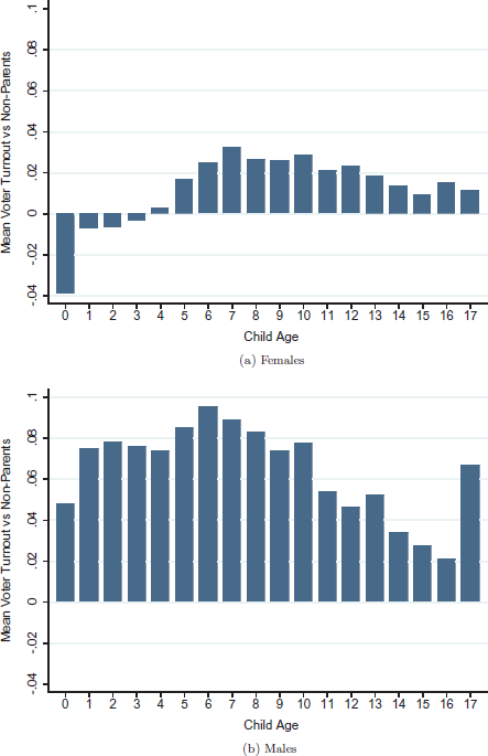
Figure 1 shows mean turnout rates for mothers (Panel (a)) versus other women and fathers (Panel (b)) versus other men by child age. Parents are included in the mean if they have and live with any child in the relevant category; for example, parents with a 1-year-old and 2-year-old child are included in the mean for both groups. As shown, mothers of infants have raw turnout rates about 4 percentage points lower than non-mothers; turnout increases with child age and mothers of older children have higher raw turnout than non-mothers. Fathers’ turnout also is higher in the presence of slightly older versus infant children, although fathers living with own children of any age have higher turnout than other men. These raw differences in turnout may be driven by a variety of characteristics besides the presence of an infant including marital status, age, or state of residence. The differences in characteristics may be especially pronounced between fathers and other men, as fathers living with their children are more likely than non-residential fathers to have characteristics associated with greater turnout such as higher educational attainment (Jones and Mosher, 2013). To examine the relationship between infants and parents’ turnout controlling for differences in observable characteristics, the following linear probability model is run:
where yi,s,t is equal to 1 if individual i in state s at time t voted, and 0 otherwise. CHILDj is a dummy variable that equals 1 if the individual has a child of age j in the household, and represent k individual characteristics that can affect voting behavior including age dummies (22 total dummies, one for each age between 18 and 39); marital status; whether voting behavior is reported by self or proxy; whether one is a naturalized citizen; race/ethnicity (non-Latino/a White, non-Latino/a Black, Latino/a, Asian, with the omitted category of “other”); duration at current residence (indicators for less than 1 year, 1–2 years, 3–4 years, with the omitted category being 5 years or longer);19 and indicators for whether the individual has at least a high school education, some college, a bachelor’s degree, and post-college education.20 State-by-year fixed effects, ηs,t, control for a variety of state-year specific factors that affect turnout such as concurrent elections for senate or governor or the competitiveness of the presidential race in a given state. Finally, ϵi,s,i is an individual error term.21 Standard errors are clustered at the state level.
Voting and children’s ages.
Note: This figure shows the mean voter turnout rates for residential parents relative to those without their own children in the household by child age as reported in the CPS-VRS. The sample includes eligible voters aged 18–39 from 1992 to 2018. Parents are included in the mean if they have and live with any child of a given age. Observations are weighted using the CPS voter supplement weights.
Table 2, columns (1) and (3), display the coefficient estimates on CHILDj (the presence of a child of age j) for women and men, respectively. The coefficients on child’s age 0–6 are shown in the table. While dummy variables for having a child of each age through 17 are included in the specifications, the full set of coefficients is not shown due to space constraints. As shown, voting rates are substantially lower among those with young children, especially infants. Relative to those without children in the household, women with infants are 3.5 percentage points (6.9%) less likely to vote and women with children ages 1–4 are about 1.5 percentage points (3%) less likely to vote. The decline is smaller in magnitude for men: those with children under 1 are 2.2 percentage points (4.8%) less likely to vote while the coefficient is smaller for a child ages 1–4 and then turns weakly positive when the child reaches age 6. This may represent increased interest in public schools when a child reaches school age (Jennings, 1979).
While the estimates in columns (1) and (3) point to a negative association between turnout and having a young child, there are potential concerns with a causal interpretation. First, conditional on own age, individuals who have young children may differ from those who do not along characteristics such as religious affiliation that in themselves affect turnout. Second, other transitions that occur around the time of a birth (e.g., cohabitation with a partner, a home purchase) may affect voting rates. To test for these confounders, I examine voting behavior the year before an individual has a child using the panel nature of the CPS. As described in Section “Data”, individuals can be identified as having a child who is “ −1 years old” if the parent is first surveyed in an election year and then has a new child in the household when surveyed 9–15 months later. Individuals with an infant and those one year out from having a child are likely similar in unobserved characteristics. Furthermore, many transitions such as marriage or home purchases may already have occurred about a year before the birth of a child. As shown in columns (2) and (4), there is no association between having a child in the next year and voter turnout, providing evidence that the “infant/young child penalty” observed is causal and not driven by differences in unobserved characteristics or other life transitions occurring around the same time.
Voting and children’s ages.
| Females | Males | |||
|---|---|---|---|---|
| (1) | (2) | (3) | (4) | |
| Child next year (age −1) | 0.002 | 0.003 | ||
| (0.007) | (0.008) | |||
| Child under age 1 | −0.035 | −0.035 | −0.022 | −0.022 |
| (0.004) | (0.004) | (0.004) | (0.004) | |
| Child age 1 | −0.015 | −0.015 | −0.008 | −0.008 |
| (0.004) | (0.004) | (0.005) | (0.005) | |
| Child age 2 | −0.017 | −0.018 | −0.005 | −0.006 |
| (0.004) | (0.004) | (0.005) | (0.005) | |
| Child age 3 | −0.012 | −0.013 | −0.006 | −0.006 |
| (0.005) | (0.005) | (0.005) | (0.005) | |
| Child age 4 | −0.015 | −0.015 | −0.015 | −0.016 |
| (0.004) | (0.004) | (0.004) | (0.004) | |
| Child age 5 | 0.001 | 0.001 | −0.002 | −0.002 |
| (0.003) | (0.003) | (0.005) | (0.005) | |
| Child age 6 | 0.004 | 0.004 | 0.010 | 0.010 |
| (0.005) | (0.005) | (0.005) | (0.005) | |
| Observations | 219,981 | 219,981 | 201,194 | 201194 |
| R2 | 0.212 | 0.212 | 0.198 | 0.198 |
Note: This table shows parameter estimates and standard errors (in parentheses) from estimating Equation (1). The dependent variable equals 1 if the individual voted and 0 if she was eligible but did not vote. All regressions include state-by-year fixed effects and controls for race (White, Black, Latino, Asian), educational attainment (high school graduate, some college, college graduate, post-college), whether the individual is a naturalized citizen, whether the individual is married, whether voting behavior is reported by self or proxy, duration at current residence (indicators for less than 1 year, 1–2 years, and 3–4 years), and own age dummies. All regressions also include indicators for children ages 7–17. Columns (2) and (4) include controls for whether the individual is in the CPS sample the year following a given election and whether the individual is in the CPS for two consecutive years. Observations are weighted using the CPS voter supplement weights. Standard errors are clustered at the state level.
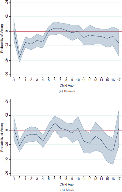
Figure 2 displays the coefficients on all child ages, providing a visual representation of the impact of young children on voting. The figure highlights the substantial decrease in turnout during the first year of the child’s life, especially for mothers.22 In terms of overall magnitude, these coefficients suggest that parenting young children could explain 0.7 percentage points (3.6%) of the approximately 20 percentage point turnout gap between younger (18–39) and older (40+) women, and 0.2 percentage points (1%) of the 24 percentage point gap between younger and older men.23 Given the small margins of victory in many recent elections, 1–4% lower turnout rates of younger versus older Americans could have substantial impacts on electoral outcomes.
Voting and children’s ages.
Note: This figure shows the coefficient estimates on having a child of each age based on estimates of Equation (1) as shown in Table 2, columns (2) and (4). All regressions include state-by-year fixed effects, controls for race (White, Black, Latino, Asian), educational attainment (high school graduate, some college, college graduate, post-college), whether the individual is a naturalized citizen, whether the individual is married, whether voting behavior is reported by self or proxy, duration at current residence (indicators for less than 1 year, 1–2 years, and 3–4 years), own age dummies, and controls for whether the individual is in the CPS sample the year following a given election and whether the individual is in the CPS for two consecutive years. The bands represent the 95% confidence intervals. Observations are weighted using the CPS voter supplement weights. Standard errors are clustered at the state level.
Heterogeneity
Which parents experience the greatest “infant penalty” in voter turnout? As noted in Section “Theoretical Overview” above, those with less financial security or childcare assistance may be less able to overcome the costs of voting. Since many demographic characteristics (especially age, education, and marital status) may affect and proxy for resources, I run the regression given in Equation (1) interacting demographic characteristics with having a child below age 1. I keep indicators for having a child of age 1, 2, etc., and individual controls such as education and race as listed above, but do not interact other children’s ages with demographic characteristics. Therefore, the coefficients on the interactions of child below age 1 with demographic characteristics can be interpreted as the difference in turnout for parents with infants relative to those without children in the household, controlling for the average effects of demographic characteristics across all individuals.
The coefficients on the interactions are shown in Table 3 for mothers and Table 4 for fathers. Focusing first on mothers of infants (henceforth called new mothers), there are substantial differences by age: new mothers under age 30 turn out at rates that are 4.7 percentage points lower than other women with similar characteristics (a 10.7% decrease on a mean of 43.9%), while new mothers aged 30-39 turn out at rates that are 2.0 percentage points lower (a 3.4% decrease on a mean of 58.2%). A Wald test indicates that the effects are statistically different with an equality p-value of 0.003. There are also differences by education and marital status. New mothers with a bachelor’s degree or more turn out at rates that are 3.6 percentage points (5.2%) lower, whereas turnout is 2.5 percentage points (7.3%) lower for new mothers with high school or less and 4.8 percentage points (9.1%) for new mothers with some college. Finally, the results indicate that lower turnout among new mothers occurs more strongly among those who are unmarried (5.2 percentage points, or 11.3%) versus married (2.8 percentage points, or 5.0%). Combined, the heterogeneity results suggest that the lower turnout rates among new mothers is especially prominent for those with fewer resources.24
Voting and infant children, heterogeneity by mother’s characteristics.
| (1) | (2) | (3) | (4) | (5) | (6) | |
|---|---|---|---|---|---|---|
| 18–29 × child under age 1 | −0.047 | |||||
| (0.006) | ||||||
| 30–39 × child under age 1 | −0.020 | |||||
| (0.006) | ||||||
| White × child under age 1 | −0.035 | |||||
| (0.005) | ||||||
| Black × child under age 1 | −0.040 | |||||
| (0.010) | ||||||
| Latina × child under age 1 | −0.024 | |||||
| (0.011) | ||||||
| Other × child under age 1 | −0.055 | |||||
| (0.021) | ||||||
| LEHS × child under age 1 | −0.025 | |||||
| (0.006) | ||||||
| Some college × child under age 1 | −0.048 | |||||
| (0.007) | ||||||
| BA or more × child under age 1 | −0.036 | |||||
| (0.007) | ||||||
| Married × child under age 1 | −0.028 | |||||
| (0.004) | ||||||
| Unmarried × child under age 1 | −0.052 | |||||
| (0.007) | ||||||
| Presidential × child under age 1 | −0.039 | |||||
| (0.006) | ||||||
| Midterm × child under age 1 | −0.031 | |||||
| (0.006) | ||||||
| Democratic state × child under age 1 | −0.043 | |||||
| (0.005) | ||||||
| Republican state × child under age 1 | −0.033 | |||||
| (0.005) | ||||||
| Swing state × child under age 1 | −0.029 | |||||
| (0.012) | ||||||
| Observations | 219,981 | 219,981 | 219,981 | 219,981 | 219,981 | 219,981 |
| R2 | 0.212 | 0.212 | 0.212 | 0.212 | 0.212 | 0.212 |
| Equality p value | 0.003 | 0.354 | 0.071 | 0.009 | 0.365 | 0.273 |
Note: This table shows parameter estimates and standard errors (in parentheses) from estimating Equation (1) with interactions of a child under 1 with various mother’s characteristics. The dependent variable equals 1 if the individual voted and 0 if she was eligible but did not vote. All regressions include state-by-year fixed effects and controls for race (White, Black, Latina, Asian), educational attainment (high school graduate, some college, college graduate, post-college), whether the individual is a naturalized citizen, whether the individual is married, whether voting behavior is reported by self or proxy, duration at current residence (indicators for less than 1 year, 1–2 years, and 3–4 years), and own age dummies. All regressions also include indicators for children ages 1–17. Observations are weighted using the CPS voter supplement weights. Standard errors are clustered at the state level.
Voting and infant children, heterogeneity by father’s characteristics.
| (1) | (2) | (3) | (4) | (5) | (6) | |
|---|---|---|---|---|---|---|
| 18–29 × Child under age 1 | −0.032 | |||||
| (0.008) | ||||||
| 30–39 × Child under age 1 | −0.014 | |||||
| (0.006) | ||||||
| White × Child under age 1 | −0.018 | |||||
| (0.005) | ||||||
| Black × Child under age 1 | −0.049 | |||||
| (0.015) | ||||||
| Latina × Child under age 1 | −0.008 | |||||
| (0.008) | ||||||
| Other × Child under age 1 | −0.071 | |||||
| (0.020) | ||||||
| LEHS × Child under age 1 | −0.014 | |||||
| (0.006) | ||||||
| Some college × Child under age 1 | −0.038 | |||||
| (0.009) | ||||||
| BA or more × Child under age 1 | −0.017 | |||||
| (0.008) | ||||||
| Married × Child under age 1 | −0.017 | |||||
| (0.005) | ||||||
| Unmarried × Child under age 1 | −0.050 | |||||
| (0.014) | ||||||
| Presidential × Child under age 1 | −0.023 | |||||
| (0.005) | ||||||
| Midterm × Child under age 1 | −0.021 | |||||
| (0.008) | ||||||
| Democratic state × Child under age 1 | −0.026 | |||||
| (0.007) | ||||||
| Republican state × Child under age 1 | −0.017 | |||||
| (0.008) | ||||||
| Swing state × Child under age 1 | −0.023 | |||||
| (0.008) | ||||||
| Observations | 201,194 | 201,194 | 201,194 | 201,194 | 201,194 | 201,194 |
| R2 | 0.198 | 0.198 | 0.198 | 0.198 | 0.198 | 0.198 |
| Equality p value | 0.126 | 0.008 | 0.120 | 0.051 | 0.871 | 0.702 |
Note: This table shows parameter estimates and standard errors (in parentheses) from estimating Equation (1) with interactions of a child under 1 with various father’s characteristics. The dependent variable equals 1 if the individual voted and 0 if he was eligible but did not vote. All regressions include state-by-year fixed effects and controls for race (White, Black, Latino, Asian), educational attainment (high school graduate, some college, college graduate, post-college), whether the individual is a naturalized citizen, whether the individual is married, whether voting behavior is reported by self or proxy, duration at current residence (indicators for less than 1 year, 1–2 years, and 3–4 years), and own age dummies. All regressions also include indicators for children ages 1–17. Observations are weighted using the CPS voter supplement weights. Standard errors are clustered at the state level.
In addition to individual characteristics, characteristics of the election itself may influence new mothers’ turnout. Notably, turnout rates tend to be higher in presidential relative to midterm elections. However, as shown in the final column, there are no significant differences in new mothers’ turnout by election type. Finally, state partisanship may influence turnout. For example, competitiveness of swing state elections may increase mobilization. I divide states into Democratic, Republican, and Swing states based on their average Democratic minus Republican presidential vote share relative to the national average share from 1992 to 2018.25 States with values above 0.05, between −0.05 and 0.05, and below −0.05 are classified as Democratic, Swing, and Republican states, respectively.26 The last column of Table 3 shows the interaction of state partisanship with the presence of an infant. As shown at the base of the table, there are no significant differences across state partisanship.27
Table 4 shows heterogeneity for fathers. Like mothers, younger, unmarried, and less educated new fathers turn out at low rates relative to those without children, although the differences across age and education groups are only marginally significant with p-values of 0.126 and 0.120, respectively. Fathers also show heterogeneity by race, with new Black fathers experiencing greater drops in turnout associated with an infant (4.9 percentage points, or 10.7%) than White fathers (1.8 percentage points, or 3.7%) or Latino fathers who do not show any significant decline in turnout. Interestingly, other races of fathers (which includes Asian, Native American, multiracial, and fathers who do not identify with other groups) also experience substantial declines in turnout. The racial differences may reflect barriers faced by Black voters such as long polling place wait times that lead to a high opportunity cost of voting, especially in the presence of parental responsibilities (Pettigrew, 2017). However, it is unclear why new Black fathers experience greater relative declines relative to White fathers while there is no significant difference present for mothers. It is also unclear why fathers of other races experience the greatest turnout declines. There are no significant differences for new fathers across election type or state partisanship.
Registration
The act of registering to vote imposes time and/or effort costs that have been shown to be a barrier to turnout, especially for young voters (Holbein and Hillygus, 2016). Examining the link between young children and registration provides insight into whether the “infant voting penalty” is primarily driven by the increased costs of registration or the increased costs of voting itself. Table 5 repeats Table 2 with registration as the dependent variable, which is given a value of 1 if the individual reports that she voted or that she did not vote but was registered and given a value of 0 if she reports not being registered to vote. Individuals are omitted from the sample if they did not know if they were registered or refused to answer the question about registration.28
Table 5 shows that the link between young children and registration rates is small in magnitude. For women, having a child under age 5 lowers registration by about 1 percentage point (1.4% on a mean of 71%), but there is no especially strong penalty for infants. For men, the coefficients on young children are generally negative but only that on a child of age 4 is statistically significant at conventional levels. These results indicate that the “infant penalty” is not primarily acting through lower registration rates. In the next section, I turn to state voting systems to examine the role of barriers such as getting to the polls on turnout rates for parents of infants.
Voter registration and children’s ages.
| Females | Males | |||
|---|---|---|---|---|
| (1) | (2) | (3) | (4) | |
| Child next year (age −1) | 0.007 | 0.011 | ||
| (0.007) | (0.008) | |||
| Child under age 1 | − 0.012 | −0.012 | −0.005 | −0.005 |
| (0.004) | (0.004) | (0.005) | (0.005) | |
| Child age 1 | −0.008 | −0.008 | −0.002 | −0.002 |
| (0.004) | (0.004) | (0.005) | (0.006) | |
| Child age 2 | −0.009 | −0.009 | −0.001 | −0.002 |
| (0.004) | (0.004) | (0.006) | (0.006) | |
| Child age 3 | −0.009 | −0.009 | −0.001 | −0.002 |
| (0.004) | (0.004) | (0.005) | (0.005) | |
| Child age 4 | −0.013 | −0.013 | −0.009 | −0.009 |
| (0.004) | (0.004) | (0.005) | (0.005) | |
| Child age 5 | −0.000 | −0.000 | −0.003 | −0.003 |
| (0.003) | (0.003) | (0.004) | (0.004) | |
| Child age 6 | 0.011 | 0.011 | 0.003 | 0.003 |
| (0.004) | (0.004) | (0.006) | (0.006) | |
| Observations | 216,025 | 216,025 | 196,086 | 196,086 |
| R2 | 0.158 | 0.158 | 0.160 | 0.160 |
Note: This table shows parameter estimates and standard errors (in parentheses) from estimating Equation (1). The dependent variable equals 1 if the individual was registered to vote and 0 if she was eligible to vote but not registered. All regressions include state-by-year fixed effects, controls for race (White, Black, Latino, Asian), educational attainment (high school graduate, some college, college graduate, post-college), whether the individual is a naturalized citizen, whether the individual is married, whether registration information is reported by self or proxy, duration at current residence (indicators for less than 1 year, 1–2 years, and 3–4 years), and own age dummies. All regressions also include indicators for children ages 7–17. Columns (2) and (4) include controls for whether the individual is in the CPS sample the year following a given election and whether the individual is in the CPS for two consecutive years. Observations are weighted using the CPS voter supplement weights. Standard errors are clustered at the state level.
State Voting Systems
Can certain state policies mitigate the negative relationship between infants and parents’ turnout? In all states, individuals are able to obtain an absentee ballot for a set of established excuses such as being on military duty or disabled, but care for an infant is not typically included as a valid excuse.29 Since the late 1980s, many states have enacted additional policies designed to allow voting at alternative times or locations. These include the following: universal vote-by-mail, wherein all individuals registered to vote are mailed a ballot and return the ballot by mail or in person; early voting, wherein individuals are able to go to a polling place for a set number of days prior to election day; permanent absentee, wherein individuals can request an “absentee” (mail) ballot for all elections with one request; and no-excuse absentee, where individuals can request an absentee ballot even without an approved excuse. There has also been an increase in non-traditional forms of registration including election day registration, which allows individuals to register and then vote on the same day and automatic voter registration, wherein all individuals are automatically registered to vote after any interaction with government agencies such as the state Department of Motor Vehicles (DMV). Figure A2 in the Appendix shows the increase in nontraditional voting and registration over time.30
Overall, these nontraditional policies enable parents to vote more easily by lowering the physical costs of going to the polls (in the case of universal vote-by-mail, permanent absentee, or no-excuse absentee), enabling them to vote at more convenient times (early voting), or allowing them to register more easily (election day registration or automatic registration). However, universal vote-by-mail provides the greatest potential benefit because it reduces physical costs without requiring additional logistical work to request an absentee ballot. Furthermore, the limited impact of infants on registration as highlighted above suggests that reforms enabling easier registration may have only a marginal effect.
Three states implemented universal vote-by-mail systems for general elections between 1992 and 2018: Oregon (in 2000), Washington (in 2012), and Colorado (in 2014).31 However, driven by the Obama campaign’s efforts in the highly competitive state, Colorado experienced widespread mobilization of younger voters 6 years before the state implemented universal vote-by-mail. This included increasing use of permanent absentee rules to mail in ballots (Johnson, 2008). Between 2004 and 2008, the fraction of voters in Colorado mailing in ballots approximately doubled from 29 to 59% according to the VRS (with rates for those ages 18–39 increasing almost threefold from 17% to 48%); therefore, it is difficult to pinpoint the timing of the vote-by-mail “treatment,” particularly for younger voters. I omit Colorado in the main results and show in Appendix Table A6 that the results are not sensitive to its inclusion. Furthermore, I show the results are robust to excluding other states with widespread use of mail-in ballots but no universal vote-by-mail programs by 2018.32
I use a design that compares voting rates across individuals within states over time. Specifically, I compare the difference in turnout between parents with infants and others within each state before and after the state adopts a universal vote-by-mail system, while controlling for national differences in voting between those with infants and others over time. The following linear probability model is used:
where MAILs,t reflects whether state s at time t has universal vote-by-mail and is an indicator for whether the individual has an infant in the home. State-by-year fixed effects (η) control for differences in turnout related to factors such as the competitiveness of the election in a given state and year. The interaction of state fixed effects (γ) and year fixed effects (δ) with having a child under age 1 account for differences in who becomes a parent across states and across time. All other variables are as defined above. I also include additional controls for universal vote-by-mail systems interacted with individual (own) age dummies to isolate the impact of vote-by-mail on parents with infants from any impacts of vote-by-mail on the age profile of voting. For example, if those who are 25 experience increased turnout as a result of universal vote-by-mail systems and are also relatively likely to have an infant, failing to control for age interacted with vote-by-mail would bias the estimate upward.
Voting systems and infant children.
| Females | Males | |||
|---|---|---|---|---|
| (1) | (2) | (3) | (4) | |
| Universal vote-by-mail × | 0.049 | 0.052 | 0.033 | 0.056 |
| Child under age 1 | (0.006) | (0.018) | (0.021) | (0.031) |
| Permanent absentee × | 0.008 | 0.008 | ||
| Child under age 1 | (0.014) | (0.015) | ||
| No-excuse absentee × | −0.005 | 0.016 | ||
| Child under age 1 | (0.012) | (0.020) | ||
| Early voting × | 0.019 | −0.011 | ||
| Child under age 1 | (0.015) | (0.023) | ||
| Election day registration × | 0.035 | 0.012 | ||
| Child under age 1 | (0.025) | (0.027) | ||
| Automatic registration × | 0.048 | -0.030 | ||
| Child under age 1 | (0.030) | (0.054) | ||
| Observations | 216,123 | 216,123 | 197,500 | 197,500 |
| R2 | 0.212 | 0.212 | 0.197 | 0.199 |
Note: This table shows parameter estimates and standard errors (in parentheses) from estimating Equation (2). The dependent variable equals 1 if the individual voted and 0 if she was eligible but did not vote. All regressions include state-by-year fixed effects, state by child under 1 fixed effects, year by child under 1 fixed effects, and controls for race (White, Black, Latino, Asian), educational attainment (high school graduate, some college, college graduate, post-college), whether the individual is a naturalized citizen, whether the individual is married, whether voting behavior is reported by self or proxy, duration at current residence (indicators for less than 1 year, 1–2 years, and 3–4 years), and indicators for children ages 1–17. They also include fixed effects for each age interacted with the voting system(s) studied in each column. Colorado is excluded in all years. Observations are weighted using the CPS voter supplement weights. Standard errors are clustered at the state level.
Table 6 displays the results. The first column indicates that universal vote-by-mail systems increase voting among women with infants by about 5 percentage points relative to other women in the state and relative to women with infants in states without universal vote-by mail systems. Interestingly, this is somewhat larger in magnitude than the association between having an infant and voter turnout from Table 2, indicating that universal vote-by-mail systems eliminate the infant penalty on women’s turnout. Column (3) provides suggestive evidence that vote-by-mail may also increase turnout among men with infants.
Since states could have adopted other policies prior to or in conjunction with universal vote-by-mail, in column (2) (respectively, column (4) for males) I control for the interaction of these other voting systems with a child under age 1. As in columns (1) and (3), I also include controls for the interaction of each voting system with age to account for their effects on the age profile of voting. If anything, the inclusion of these controls strengthens the results for females; the results remain on the margin of statistical significance for males. No other voting systems affect turnout rates for parents of infants in this regression. Table A6 in the Appendix shows the robustness of the vote-by-mail results for mothers to sample adjustments. The results for men, however, are sensitive to the sample used, and thus do not provide clear evidence on the relationship between universal vote-by-mail and turnout for new fathers.33
Although the controls in columns (2) and (4) account for reforms that states may pass in the years prior to universal vote-by-mail systems, there may be other movements within the states driving both implementation of universal vote-by-mail policies and higher turnout among women with infants. To test for this possibility, I perform an event study to explore pre-trends. I use Equation (2), interacting CHILD0 with dummies indicating the passage of time before/after the reform. As above, I also interact age dummies with the amount of time before/after the reform to account for changes in the age profile of voting. I also include the full set of controls for the presence of other state voting systems (as in columns (2) and (4) of Table 6) and age dummies interacted with these. Because turnout rates are substantially different between midterm and presidential elections, I group the elections together into 4-year periods.
The event study coefficients and 95% confidence intervals are shown in Figure A3 in the Appendix, with the period 2–4 years before the implementation of universal vote-by-mail set to zero. The panels do not suggest evidence of pre-trends for new parents of either gender before the passage of vote-by-mail reforms. After the reforms, panel (a) shows immediate increases in new mothers’ turnout. Panel (b) indicates that increases in new fathers’ turnout occur 4–6 years after the reforms, possibly indicating a later utilization of this system.
These results indicate that the act of physically going to the polls may pose a barrier to political participation for those with infants, especially mothers. However, the ability to vote at an alternative location does not increase mothers’ turnout if it requires additional logistical costs such as requesting an absentee ballot. This suggests that states concerned about the barriers faced by new mothers may be able to mitigate them with universal vote-by-mail systems.
Conclusion
Voting is a fundamental act of democracy. As a result, it is important for governments to know how life events such as the birth of a child affect parents’ political engagement and which policies can mitigate any negative effects. This paper provides a first exploration of the impact of infant children on voting in the United States. Relative to those without children, women with an infant in an election year are 3.5 percentage points (6.9%) less likely to vote and men are 2.2 percentage points (4.8%) less likely to vote. There is no significant association between turnout and having a child next year, suggesting that the negative link between infants and turnout is causal. This effect is particularly strong among young, unmarried, and less-educated parents and Black fathers and fathers of other (non-White, non-Latino) races and ethnicities. Furthermore, universal vote-by-mail mitigates these negative effects for mothers.
This paper contributes to a nascent literature on the impact of children on voter turnout, providing analysis for U.S. context and an exploration of the impact of nontraditional voting on the “infant penalty.” Future projects could further explore how other state policies surrounding voting (such as poll opening and closing times) interact with parental responsibilities to affect voter turnout.
Effects of young children on turnout have recently been studied in Italy (Bellettini et al., 2019) and Denmark and Finland (Bhatti et al., 2019), although these reflect a different social and political context than that of the United States.
A separate small literature examines the correlation between having children of any age and voter turnout. In the United States, Wolfinger and Wolfinger (2008) and Arnold (2013) document a negative association between turnout and children under 18 in the household and turnout and children under 6 in the household, respectively. Welch (1977) highlights the association between women’s family responsibilities and lower turnout in the historical U.S. context and Jennings (1983) explores the relationship between gender roles and turnout across countries. Focusing on Italy, Quaranta (2016) finds a negative association between turnout and children under 5 for women (and a positive association for men). Using a dataset covering 5 countries (Canada, France, Germany, Spain, and Switzerland), Santana and Aguilar (2019a,b) highlight that children are not associated with higher costs of voting overall but are associated with higher costs for women relative to men.
In a report from Save the Children (2015), the United States ranked 33rd among countries on a mother’s index incorporating data on risk of maternal death, under-5 mortality of children, years of schooling, per capita income, and political participation of women in national governments. This was low relative to other developed countries including Finland (2nd), Denmark (4th), and Italy (12th).
There is mixed evidence on turnout effects of early voting (Burden et al., 2014; Gronke et al., 2007; Kaplan and Yuan, 2020).
Ko et al. (2017) examine rates of postpartum depression across 13 U.S. states, finding rates ranging from 8% to 20% in 2012. See Pacheco and Fletcher (2015) and Ojeda and Pacheco (2019) for the link between health and political participation.
For example, Baicker and Finkelstein (2019) find that receipt of Medicaid from a government expansion increased voter turnout in Oregon in 2008.
Using data from 1992 also allows two full election cycles prior to the earliest universal vote-by-mail reform in Oregon in 2000 (which will be examined in Section “State Voting Systems’’).
In both the basic monthly survey and the VRS, one person often reports data for all individuals in the household. Regressions in this paper control for whether voting behavior was reported by oneself or another person in the household.
Data on official turnout rates is obtained from the United States Election Project. See McDonald (2019).
The adjustments are downloaded from McDonald (2020). The results are also robust to coding “voted” as 1 if the individual voted in the most recent election and 0 if she was eligible but did not vote, did not know, or refused to answer the question as in Burden et al. (2014), reported in Table A3 in the Appendix.
I exclude from the sample those who answer the voting question in November and then are interviewed and have a new child the following December, January, or February. This group does not provide an appropriate counterfactual for parents of infants, given the physical difficulties associated with voting in the final trimester. In a regression, this group experiences a decrease in turnout of 4.1 percentage points (females) and 3.0 percentage points (males) relative to those without children. Those who are not interviewed in December, January, and February but have a child the next year are included in the “child age −1” group, since it cannot be observed whether these individuals are in their third trimester in November. The results are similar if the sample is restricted to those interviewed for the first time in November of an election year (and thus likely to be interviewed through the February after the election year).
There will be missing information on “child age −1” for two groups: 1) those who are in the second year of the CPS in the election year and 2) those who are in the first year of the CPS in the election year but not followed into the next year. I include dummy variables for both of these groups. Table A4 in the Appendix shows the results are similar if I exclude both of these groups from the regressions.
In the CPS sample, less than 2% of women and less than 4% of men of any age over 39 have an infant (child under age 1) in the household.
In 2004, about 62% of children lived with two biological parents or two adoptive parents, and almost 29% lived with their biological or adoptive mother but not biological or adoptive father (Kreider, 2004).
If two mothers are listed for a given child, both are included in the sample of women. The same procedure is used for fathers.
Note that this is slightly higher than the official turnout statistics, as discussed at the beginning of this section. The results are robust to re-weighting individuals to match aggregate official state-by-year turnout rates using the correction proposed by Hur and Achen (2013), as shown in Table A2 in the Appendix.
The married variable takes a value of 1 if the individual reports she is “married, spouse present’’ or “married, spouse absent” and takes a value of 0 if the individual is separated, divorced, widowed, or never married. Although those who are separated are technically married, they are unlikely to be living with or having political discussions with a spouse. Assistance with voting logistics as well as political discussions with a spouse have been suggested as important mechanisms driving higher turnout among married people (Wolfinger and Wolfinger, 2008).
Table A5 in the Appendix shows the relationship between the number of infants and voter turnout.
In cases where there is no information on duration at residence, the former indicators are all given values of 0 and a dummy for “missing” is given a value of 1.
These are standard controls in models of voter turnout, see, e.g., Burden et al. (2014).
Using a linear probability model provides the advantage of ease in interpretation. Average marginal effects from a probit model are similar to the estimates obtained from OLS. These are available upon request.
Results with adjustments to individual weights as recommended in Hur and Achen (2013) are in Appendix Table A2. Results with an alternative construction giving a value of 0 to those who did not answer the voting question (rather than excluding them) are available in Table A3. In both, coefficient estimates for a child under 1 remain negative and significant and the coefficient on “child age −1” remains insignificant for both genders.
The 0.7 estimate for women is obtained by multiplying the fraction of women with a child of each age between 0 and 4 (see Table 1) by the corresponding coefficients in the second, third, fourth, fifth, and sixth rows of column (2) in Table 2. These products are then added together. The 0.2 estimate for men is obtained by multiplying 6% and 5% by the coefficients in the second and sixth rows of column (4) in Table 2, respectively, and then adding the products together.
Table A5 in the Appendix shows heterogeneity by infant birth order (column (1) for women and (3) for men) and number of children under age 1 (columns (2) and (4)). For mothers, first- and second-born infants are associated with greater declines in turnout than third-born and higher-order infants. There is also suggestive evidence of greater declines for women with multiple infants, although the point estimates are imprecise. Interestingly, the point estimates are slightly larger than Dahlgaard and Hansen (forthcoming), who find that an additional child caused by the birth of twins in Denmark decreases mothers’ turnout by an additional 1.6−3 percentage points.
This methodology is similar to that used in the Cook Partisan Voter Index to calculate partisanship for congressional districts based on the prior two presidential elections.
Data from the MIT Election Data and Science Lab (2017) are used to obtain information on presidential election results by state. The Democratic states (and districts) are California, Connecticut, Delaware, the District of Columbia, Hawaii, Illinois, Maine, Maryland, Massachusetts, Minnesota, New Jersey, New York, Oregon, Rhode Island, Vermont, and Washington. The Swing states are Colorado, Florida, Iowa, Michigan, Nevada, New Hampshire, New Mexico, Ohio, Pennsylvania, Virginia, and Wisconsin. The Republican states are Alabama, Alaska, Arizona, Arkansas, Georgia, Idaho, Indiana, Kansas, Kentucky, Louisiana, Mississippi, Missouri, Montana, Nebraska, North Carolina, North Dakota, Oklahoma, South Carolina, South Dakota, Tennessee, Texas, Utah, West Virginia, and Wyoming.
The difference in these results and the positive impact of universal vote-by-mail shown in Section “State Voting Systems” may reflect the fact that, prior to the 2020, the accessibility of non-traditional voting varied across both Democratic and Republican states. For example, in 2012, the states with the highest rates of non-traditional voting were Oregon, Washington, Colorado, Nevada, Arizona, Texas, North Carolina, Montana, New Mexico, and Tennessee (DeSilver and Geiger, 2016). One state that implemented universal vote-by-mail (Colorado) was a Swing state over the period 1992–2018 while two (Oregon and Washington) were Democratic states.
In more recent years, it is more difficult to assess registration separately from voting since increases in election day registration make the combination of these activities more likely.
Data on absentee and mail voting systems was provided through personal correspondence with the Pew Research Center based on a published report (DeSilver and Geiger, 2016) and from the National Conference of State Legislatures (2018). I make one change to Pew’s classifications. Although Washington did not adopt vote-by-mail statewide until 2012, all but one county used universal vote-by-mail in 2010 and numerous counties used universal vote-by-mail between 2006 and 2010. King County, which is the most populous county in the state and includes Seattle, switched to fully vote-by-mail elections in 2009. Therefore, I classify Washington as a universal vote-by-mail state rather than a permanent absentee and no-excuse absentee state from the 2010 election forward. Results (available upon request) are robust to classifying Washington as a universal vote-by-mail state beginning in 2012. Results are also robust to assigning vote-by-mail status to Washington residents based on county between 2006 and 2012, with King county residents assigned universal vote-by-mail status from the 2010 election forward and Clark, Kitsap, Skagit, Snohomish, Spokane, Thurston, Whatcom, Yakima, and unidentified county residents assigned universal vote-by-mail status from the 2006 election forward. The results are also robust to excluding Washington state from the analysis (see Table A6 in the Appendix). Data on election day registration and automatic voter registration comes from the National Conference of State Legislatures (2020, 2021).
These dates refer to the first general election in which the state had a universal vote-by-mail system.
These include Arizona, California, Montana, and Utah which, according to the VRS, had 60, 49, 49, and 42% of voters, respectively, mail in ballots from 2008 to 2018. Since 2012 in Utah and 2018 in California, some counties have conducted exclusively vote-by-mail elections.
The results for mothers are robust to the inclusion of Colorado (column (1)) and the omission of states with high vote-by-mail participation but without universal vote-by-mail including Arizona, California, Montana, and Utah (column (2)). They are also robust to only examining the reform in Oregon (column (3)). Oregon’s reform is the cleanest over the period as less than half of voters used absentee options in 1996 and no county had implemented vote-by-mail before the statewide reform effective in 2000. Note that columns (2), (3), (5), and (6) do show a positive effect of election day registration for new parents of both genders, suggesting that election day registration may be helpful in states without substantial use of absentee voting.
