


Bridges are critical transport link that are frequently impacted by flooding. Despite substantial research on the risk of bridges to floods, there is a knowledge gap regarding restoration modelling, as there are very few available in the literature and most of them rely on expert elicitation. This paper provides the first restoration models that are based on documented cases and real data. The restoration of a portfolio of bridges that were damaged or collapsed during the 2015 Cumbrian floods in the UK was analysed. The purpose of this exercise was to develop a methodology that can be replicated to other case studies for facilitating resilience modelling for bridges affected by floods. Published restoration and recovery modelling techniques were used to establish a repeatable way of analysing a large portfolio of bridges in one model, offering valuable insights into the specific challenges and strategic considerations essential for effective post-flood recovery. This approach evaluates the serviceability levels during the restoration process and identifies key factors influencing restoration outcomes, underscoring the need for evidence-based restoration models to enhance infrastructure resilience against future flood events.
1. Introduction
Bridges are critical transport infrastructure assets, as they are essential in connecting communities around the world. However, with the ever-increasing effects of global warming leading to more frequent natural disasters, such as more frequent and intense floods (Chen et al., 2023), it is important to ensure that bridges are built to withstand these (once-infrequent) events and to model recovery after extreme events as a means to quantify their resilience. One way to do develop recovery models is to reflect and learn from past disasters and to establish what enabled and what prevented quick recovery, to ensure that corrective measures can take place before a similar, or worse, situation were to occur again.
During 5–6 December 2015, Storm Desmond brought devastation and flooding throughout Cumbria, in northwest England, cutting communities off for varied lengths of time (Met Office, 2015a). Storm Eva landed just a few weeks afterwards, on 24 December, worsening the situation in northern England (Met Office, 2015b). While these floods are often referred to as being 1-in-100-year floods, the 2009 flooding event, which also caused significant damage to Cumbria, tends to indicate that these low-probability flooding events are becoming more and more common (Chiverrell et al., 2015). The 2009 floods were significant in England’s recent history, with record rainfall of 316 mm in 24 h causing flash flooding in Cockermouth and Workington, the highest seen before the 2015 floods broke this record at 341.4 mm in 24 h (hrwallingford, 2015). It is estimated that the 2015 floods brought economic damage of £1.6 billion and the 2009 floods resulting in an estimated £276 million of damage, the difference being likely down to the geographical spread affecting a larger area of towns and villages (BBC, 2010; EA, 2018).
The aim of this work was to build on data acquired from the 2015 Cumbria floods and further analyse the extensive damage these floods brought upon the entire County of Cumbria, by analysing the restoration responses of the local authorities. The focus is the response and recovery of bridges.
Although reports have examined the overall impact of the floods on the region, a detailed investigation into the long-term effects of infrastructure restoration, particularly on the most impacted among the 792 affected bridges, remains unexplored, with the most recent and most detailed assessment being the impact assessment conducted by Cumbria County Council (CCC) (CCC, 2018a).
Documented and reported restoration/recovery tasks and endeavours after the flood were used to provide evidence-based models for post-flood bridge restoration. Bridge restoration efforts of the authorities over the past 8 years were also analysed to determine the extent and efficiency of restoration efforts of the chosen restoration decisions.
1.1 Development of evidence-based restoration models
There are very few methods for measuring the restoration of bridges after a flooding event. Mitoulis et al. (2021) developed a recovery model for bridges affected by flooding-related hydraulic actions such as scour. This model addressed the need to measure the flood resilience of bridges and focused specifically on the need to incorporate both bridge reinstatement (traffic capacity) models and restoration (structural capacity) models to establish recovery models. The methodology involves assessing bridge hazards, determining robustness and calculating damage levels (DLs) based on damaged components and fragility models. Reinstatement and restoration models are then developed using previously completed restoration task information. Further information-gathering tasks are needed as the costs associated with DLs, shown in the report (Mitoulis et al., 2021), indicate that lower DLs correspond to lower costs, with deep foundations incurring higher costs than spread foundations. Restoration tasks were estimated by means of expert elicitation using a questionnaire (Mitoulis and Argyroudis, 2021) and the findings are presented in Table 1. While Table 1 is useful in estimating how long it takes to complete certain restoration tasks – something that can be compared with actual case studies – it misses tasks that were not found during the survey, hence the addition of R24. This results in a generalised approach that may not be accurate to cases with unforeseen/unusual situations. After this, all the information acquired is combined to establish recommendations and adaptations, for the quantification of the resilience of the bridges, developing further decision making or reflection on how restoration occurred. Comparison with real-world instances of the restoration tasks being completed will help establish the accuracy of the results from this survey and would also help increase the database of damage against cost.
Duration of restoration tasks and weighting factors per DL (adapted from (Mitoulis et al., 2021))
| Code | Restoration task | Duration: days | Weighting factor | ||||||
|---|---|---|---|---|---|---|---|---|---|
| Minimum | Maximum | Mean | Standard deviation | Minor | Moderate | Extensive | Severe | ||
| R0 | No action required | n/a | n/a | n/a | n/a | n/a | n/a | n/a | n/a |
| R1 | Armouring countermeasures and flow-altering/cofferdam | 5.6 | 24.8 | 15.2 | 13.4 | 0.7 | 0.8 | 0.9 | 1 |
| R2 | Temporary support per pier | 3.2 | 9.2 | 6.2 | 4.2 | 0.7 | 0.8 | 0.9 | 1 |
| R3 | Temporary support of one abutment | 3 | 10 | 6.5 | 4.6 | 0.7 | 0.8 | 0.9 | 1 |
| R4 | Temporary support of one deck span/segment (midspan or support) | 3.6 | 10.8 | 7.2 | 3.9 | 0.7 | 0.8 | 0.9 | 1 |
| R5 | Repair cracks and spalling with epoxy and/or concrete | 3.4 | 19 | 11.2 | 13 | 0.5 | 0.7 | 0.85 | 1 |
| R6 | Realignment and/or levelling of pier | 12 | 29.8 | 20.9 | 23.6 | 0.5 | 0.7 | 0.85 | 1 |
| R7 | Realignment of bearings | 2.8 | 10 | 6.4 | 6.8 | 1 | 1 | 1 | 1 |
| R8 | Jacketing or local strengthening (pier or abutment or foundation) | 11.4 | 35 | 23.2 | 30 | 0 | 0.4 | 0.7 | 1 |
| R9 | Jacketing or local strengthening (deck) | 13.8 | 32.8 | 23.3 | 23.3 | 0 | 0.4 | 0.7 | 1 |
| R10 | Realignment of deck segment | 8.2 | 18.2 | 13.2 | 17.9 | 0.5 | 0.7 | 0.85 | 1 |
| R11 | Erosion protection measures | 6.8 | 16.3 | 11.5 | 6.4 | 0.7 | 0.8 | 0.9 | 1 |
| R12 | Rip-rap and/or gabions for filling of scour hole and scour protection | 6 | 23.4 | 14.7 | 13.5 | 0.7 | 0.8 | 0.9 | 1 |
| R13 | Removal of debris | 2.9 | 7.4 | 5.2 | 4.7 | 0.7 | 0.8 | 0.9 | 1 |
| R14 | Ground improvement per foundation | 11.2 | 32 | 21.6 | 21.8 | 0.7 | 0.8 | 0.9 | 1 |
| R15 | Installation or retrofitting of deep foundation system | 33.8 | 66 | 49.9 | 49.3 | 1 | 1 | 1 | 1 |
| R16 | Extension of foundation footing | 20.8 | 46 | 33.4 | 32.1 | 1 | 1 | 1 | 1 |
| R17 | Reconstruction/replacement of the abutment and wingwalls | 31 | 72 | 51.5 | 41.1 | 1 | 1 | 1 | 1 |
| R18 | Reconstruction/replacement of the pier | 42 | 78 | 60 | 44.3 | 1 | 1 | 1 | 1 |
| R19 | Temporary support and replacement of bearings | 3.8 | 9.4 | 6.6 | 3.8 | 1 | 1 | 1 | 1 |
| R20 | Replacement of backfill and approach slab and mud jacking | 12 | 32 | 22 | 11.5 | 1 | 1 | 1 | 1 |
| R21 | Replacement of expansion joint | 2 | 7.2 | 4.6 | 3.1 | 0.5 | 0.7 | 0.85 | 1 |
| R22 | Demolition/replacement of a deck span/segment | 22.2 | 51 | 36.6 | 23.2 | 1 | 1 | 1 | 1 |
| R23 | Demolition/replacement (part) of the bridge | 88.8 | 334 | 211.4 | 133.8 | 1 | 1 | 1 | 1 |
| R24 | Customised task | — | — | — | — | — | — | — | — |
The weighting factors in Table 1 adjust the restoration task durations based on the DL. These factors help to account for varying levels of damage, with lower values shortening task durations and higher values representing more severe damage that requires full-time allocation.
Kameshwar et al. (2020) described an effective way of quickly establishing probabilities for bridge or lane closures, based on decision tree diagrams, but did not offer detail beyond this – something this work aimed to address.
Bocchini and Frangopol (2012), Karamlou and Bocchini (2017) and Gidaris et al. (2017) principally focused on a broader range of theoretical models and frameworks on earthquake impacts, systemic probabilistic models and multi-hazard assessments. However, in this work, a specific flooding event was considered as a case study to develop a practical, applicable restoration model.
Godazgar et al. (2023) proposed a method of quantifying hazard resiliency that completes fragility analysis using both restoration and recovery information, using detailed restoration data from a case study of Chemin des Dalles Bridge, in Canada. Information regarding restoration analysis outlines the importance of knowing what restoration tasks were undertaken before being able to obtain further information, such as resilience. In this report, a useful example of a resilience curve is used, like those produced by Mitoulis et al. (2021), which is key to visually representing simplified but accurate resilience models. The report outlines how restoration information can be derived from idle time and restoration tasks, where restoration tasks comprise all the information involving the design and reconstruction of damaged components. It also outlines the uncertainty of how long tasks take and how challenging it is to accurately represent specific areas of restoration. The report provides some key methods and ideas for analysing the resilience of a specific bridge, but it is very challenging and time-consuming to do this in a large-scale case study for more than a few bridges.
Resilience is crucial for bridges as they are vital infrastructure in transportation networks. Resilience ensures that bridges can withstand and recover from disasters, minimising social and economic disruption while strengthening overall community resilience.
Loli et al. (2022) used a GIS-based approach to assessing flood risk. The work started with assessing DLs, such as for a set of Greek bridges affected by Cyclone Ianos in September 2020 (Loli et al., 2023). This was completed using images and data from the work of Zekkos et al. (2020), ranking the bridges’ DLs from 1 to 5 (1 is defined as having no damage and 5 is failure).
By focusing on the 2015 floods in Cumbria, another geographic location can be added to locations with given DLs, helping to expand the library of assessed global bridges.
Some other useful papers relating to this include those of Zhang et al. (2017) and Zhang et al. (2022). These papers offer a differing insight into post-earthquake analysis and provide insights into disaster recovery of infrastructure, useful for this paper.
It should also be mentioned that other recent contributions to bridge resilience methodologies have advanced our understanding of post-disaster recovery. For example, research on the seismic resilience of bridges, using both traditional and geotechnical seismic isolation systems, has demonstrated how these technologies improve structural performance during earthquakes, enhancing recovery speed and reducing long-term disruptions (Forcellini, 2023). A recent study also compared pre- and post-seismic design considerations in moderate seismic zones, focusing on the fragility assessment of multi-span bridge classes (Ramanathan et al., 2012). The findings highlight how updated seismic design standards improve the resilience of bridges by reducing their vulnerability to damage, further advancing our understanding of post-disaster recovery strategies for various bridge types.
1.2 Reports on the 2015 Cumbria floods
Reports are available regarding the 2015 Cumbrian floods that offer highly useful information regarding Storm Desmond. However, they do not offer detailed information regarding combining and analysing multiple bridges and their data together. In 2018, CCC released an impact assessment report detailing many of the areas in which impacts were seen throughout Cumbria during and following the 2015 floods (CCC, 2018a). The 66-page assessment provides insightful information regarding impacts on the various communities inside Cumbria; however, the key area of interest in this document is the section ‘Impact on infrastructure’ (pp. 18–34). Key information makes clear the sheer number of bridges affected – 30 bridges were defined as having ‘significant damage’ and 42 bridges were ‘structurally and functionally impaired’. The report outlines how a repair programme was put together based on measurable socio-economic impacts and this report was then used to prioritise further works.
The CCC impact assessment did not provide specific scores for individual bridges, therefore a direct comparison between their results and the findings of this work is not possible. The report also failed to provide all the information on the bridges and footbridges, leaving some big gaps in the study. Key engineering information can be found in the work of Mathews and Hardman (2017), which highlights how important data was collected by the 21st Regiment of Royal Engineers in the immediate aftermath of the floods to establish which bridges were safe to open – focusing, initially, on the 120 most strategically important crossings. This was input into an asset spreadsheet reportedly called Operation Shaku – District Tracker, using red, amber and green categories (Hugh and Carolyn, 2018). However, despite thorough research, the ‘Operation Shaku’ document remained inaccessible. Consultants and divers were then brought in to complete more detailed inspection reports of the bridges coded as red or amber, using a simplified version of the Inspection Manual for Highway Structures (HA, 2007a, 2007b).
Further on in the report, case studies on some of the worst affected bridges (Pooley, Eamont, Brougham, Sprint and Victoria) are laid out. Highly detailed information such as scour estimation parameters is included for these five bridges as well as key background information. The document, however, does not provide information on how long it took for restoration to occur and omits data for the hundreds of other bridges.
1.3 Aim and objectives of this work
The aim of this study was to use evidence from a flooding event to establish restoration models to understand the level of serviceability (by evaluating the performance shown in the restoration models), to determine the bridge’s ability to restore service to original levels and to understand the parameters of restoration modelling (time, resources, tasks, cost, patterns of damage and recovery) in order to provide a comprehensive understanding of the restoration process.
2. Methodology
Before starting any analysis, establishing a case study is essential. In this work, the floods in Cumbria in December 2015 were selected, but the following steps should apply to other case studies involving bridge restoration.
After establishing the case study, the first step is to list the bridges that were involved in the case study and gather as much information as possible. This involves using various sources to establish, on a case-by-case basis, the condition of each individual bridge. If there are many bridges identified in the case study, it is more important to focus on those with the greatest damage or the greatest socio-economic impacts, as these will tend to yield more information. Important data includes
bridge name and location
time of the bridge closure/opening following the disaster
capacity of the bridge (e.g. pedestrians only or maximum tonnage) at times during/following assessment/restoration,
design elements of the bridges (e.g. use of piles, piers, culverts)
damage sustained to the bridge; primarily initial findings, but any information up until complete restoration is useful
restoration tasks completed.
The next step is to use the data on when the bridges opened and closed and the traffic capacity data to establish traffic reinstatement models of traffic capacity against time. This will be essential in visually differentiating the bridges in terms of how long they took to reopen and will help understand the accessibility of the bridges over time. Table 2 shows the percentages that can be used when specific scenarios occur on different road types. The selected road types reflect a range of traffic demands, from critical national routes to local and pedestrian access. A roads connect major towns and cities and handle significant traffic, B roads serve smaller towns, C roads are minor local routes and unclassified and footbridges are the least trafficked, often serving rural or isolated areas. This variety ensures a comprehensive assessment of bridge recovery across infrastructure of varying importance.
After this, the next stage is to ensure that all bridges have been categorised by their DL, by rating the bridges from 1 to 4 (Table 3). The DLs should be decided at the time each structure was most affected. If complete information is not available, then acquiring even extracts of information is useful in making accurate estimates and assumptions because, when categorising the bridges by DL, it is essential to consider the available methods in the literature for defining these DLs. In the context of flood resilience for bridges, Mitoulis et al. (2021) developed restoration models to quantify the resilience of bridges impacted by hydraulic actions such as scour. Their framework uses damage assessments and restoration tasks to develop recovery models that can estimate the time and effort required for restoring bridge functionality. This approach aligns with the goals of this paper, which also focuses on using real-world restoration data to model resilience after flood events. Additionally, Karamlou and Bocchini (2017) developed restoration functions for damaged bridges, focusing on probabilistic models to predict recovery timelines and costs. Similarly, Zhang et al. (2022) presented emergency inspection routing for bridges after earthquakes, offering additional methods for assessing damage states and recovery efforts.
The categorised bridges are then combined with matching time data to establish what the minimum, maximum and mean times were in restoring the bridges to full capacity. This data can be used to plot idle time graphs to establish how the severity of bridge damage bridges correlates with restoration time. Idle time graphs are then taken from the first point the bridge could be used by vehicles (or pedestrians in the case of footbridges), not when they returned to 100% capacity. However, if the bridge opened and closed again for a significant amount of time (say more than a month) due to damage from the floods, the final reopening time is used.
Finding the most affected design elements of the bridges is useful in establishing common patterns and the tasks required. When combining this information with other data, a wider picture of the level of serviceability of the bridges will become clearer, helping achieve the objectives set out.
Data on costs and available resources is used to complete graphs that establish how the DLs of bridges impact the costs and resources used; however, this data may be limited in comparison with other data as this information may not have been published, in detail, by the local authorities or owners of the bridges.
Once this is complete, all the information can be used to help establish/conclude where the priorities of the local authorities rested and establish why certain decisions were made. This is done on both a bridge-by-bridge basis as well as looking at the whole study, with the objective of understanding what comes with restoration.
Figure 1 provides a visual summary of the steps described in this section, from data collection and bridge classification to the development of traffic reinstatement models and restoration time analysis. It serves as a guide to the methodology used in this study.
Traffic reinstatement percentages
| Scenario | Traffic reinstatement: % | ||||
|---|---|---|---|---|---|
| Motorways | A roads | B roads | C and unclassified roads | Footbridges | |
| Full capacity | 100 | 100 | 100 | 100 | 100 |
| Very high weight restrictiona | 70 | 75 | 80 | 85 | N/A |
| Weight restrictionb | 60 | 65 | 70 | 70 | N/A |
| Pedestrian only | N/Ac | 5 | 5 | 5 | 100 |
| One laned | 40 | 40 | 45 | 50 | N/A |
| One laned and weight restriction | 20 | 30 | 35 | 45 | N/A |
| Reduced speed limit | 55 | 70 | 75 | 80 | N/A |
| Height limite | 65 | 70 | 75 | 80 | N/A |
| Width limite | 65 | 70 | 75 | 80 | N/A |
| Closed | 0 | 0 | 0 | 0 | 0 |
For very heavy goods (e.g. 32 t maximum)
For heavy goods (e.g. 3.5 t maximum)
Pedestrians unable to use motorway, aside from maintenance workers
Of carriageway open (e.g. use of traffic control measures on single carriageway (two traffic lanes))
Primarily affecting oversized vehicles
Definition of DLs
| DL | Severity of damage | Description |
|---|---|---|
| 1 | Minor | Either no damage or minor structural issues that have negligible impact on the bridge’s functionality or safety |
| 2 | Moderate | Noticeable structural or functional impairments that still allow for the bridge’s general use, possibly with some limitations |
| 3 | Significant | Damage severely affecting the bridge’s structural integrity or functionality, potentially necessitating partial or complete closure or the imposition of weight limits |
| 4 | Severe | Extensive structural damage compromising the bridge’s safety and functionality, making it likely unsafe for regular use. The bridge may require closure or very limited access until significant repairs or reconstruction are undertaken |
 The flowchart starts with choosing a case study. It then moves to listing all relevant bridges affected by the case study and identifying key features such as closure dates and reopening stages. Next, traffic reinstatement models are completed using traffic percentages laid out in Table 2, followed by establishing damage levels of the bridges before and during restoration. A decision point asks whether the damage levels are defined by available sources. If they are not defined, available information such as descriptions and images is used to determine the damage level of each individual bridge. If they are defined, idle time graphs are plotted using time data and available damage levels. After this step, additional information is gathered, including restoration costs, resources used and tasks completed. The importance of the bridges is then estimated based on factors such as daily traffic use or ease of accessing alternative routes. Graphs and figures are completed to compare compiled information and identify the bridges and elements most affected during restoration. The process concludes by establishing what was done well during restoration, explaining why certain decisions were made.
Flowchart of the proposed methodology for the generation of evidence-based restoration models for decision making
The flowchart starts with choosing a case study. It then moves to listing all relevant bridges affected by the case study and identifying key features such as closure dates and reopening stages. Next, traffic reinstatement models are completed using traffic percentages laid out in Table 2, followed by establishing damage levels of the bridges before and during restoration. A decision point asks whether the damage levels are defined by available sources. If they are not defined, available information such as descriptions and images is used to determine the damage level of each individual bridge. If they are defined, idle time graphs are plotted using time data and available damage levels. After this step, additional information is gathered, including restoration costs, resources used and tasks completed. The importance of the bridges is then estimated based on factors such as daily traffic use or ease of accessing alternative routes. Graphs and figures are completed to compare compiled information and identify the bridges and elements most affected during restoration. The process concludes by establishing what was done well during restoration, explaining why certain decisions were made.Flowchart of the proposed methodology for the generation of evidence-based restoration models for decision making
3. Results
3.1 Data gathering
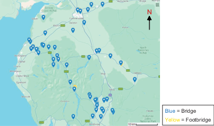
Using the available information, the most affected bridges were identified. This data came primarily from a freedom of information request regarding local bridges (CCC, 2016a). Figure 2 shows the most affected bridges from the 2015 floods. This map is useful in highlighting just how widespread the damage was across Cumbria. It also proved to be a useful tool in comparing the data found with the limited public information available. A map of closed bridges on 16 December (CCC, 2018a) was a key resource in establishing that Figure 2 shares many similar locations of some of the worst-hit bridges.
3.2 Recovery progress by road classification
From the 57 chosen bridges, 13 were on A roads, six on B roads, 20 on C roads and 18 on unclassified roads. Figure 3 shows an idle time graph of these grouped bridges and when they were opened. Figure 3 shows a correlation – the bridges that opened first being were primarily those on routes of higher importance and traffic demand, despite some outliers, such as C roads primarily having smaller and more easily repairable designs.
 The x axis shows route types A Road, B Road, C Road and Unclassified road. The y axis shows opening date from December 05, 2015 to February 21, 2024. Maximum opening date is August 02, 2019 for A Road, October 23, 2020 for B Road, June 01, 2019 for C Road and March 20, 2024 for Unclassified road. Mean opening date is April 11, 2016 for A Road, November 09, 2016 for B Road, July 13, 2016 for C Road and September 30, 2017 for Unclassified road. Minimum opening date is December 05, 2015 for all route types.
Plot of opening date against route/road type
The x axis shows route types A Road, B Road, C Road and Unclassified road. The y axis shows opening date from December 05, 2015 to February 21, 2024. Maximum opening date is August 02, 2019 for A Road, October 23, 2020 for B Road, June 01, 2019 for C Road and March 20, 2024 for Unclassified road. Mean opening date is April 11, 2016 for A Road, November 09, 2016 for B Road, July 13, 2016 for C Road and September 30, 2017 for Unclassified road. Minimum opening date is December 05, 2015 for all route types.Plot of opening date against route/road type
The major outlier of the unclassified roads is primarily due to Broad Head Bridge (U5291) not reopening at the time of writing. For B roads, the choice of using the fully reopened date of Pooley Bridge in 2020 instead of the 2016 opening date of the temporary bridge resulted in a higher mean than expected but, given the time to dismantle the temporary bridge and reconstruct the new permanent bridge, which resulted in a period of over 1 year without any road traffic, choosing the earlier date would be inappropriate. Similarly, Middleton Hall Bridge (A683) had a period of over a month in 2019 without any traffic, making it inappropriate to use the 2016 date. If both Pooley and Middleton Hall’s earlier dates were used, a much smoother mean line would be visible.
3.3 Traffic reinstatement
Plotting the data was the important next step. A traffic reinstatement model can be used to show traffic capacity against time. The traffic reinstatement model was applied to illustrate the progression of traffic capacity restoration over time. This model was chosen as it provides a clear and quantifiable way to measure how quickly the bridges returned to service, which is essential for evaluating the recovery process and the accessibility of the region following the floods.
As illustrated in Figures 4, 5 and 6, for most of the analysed bridges, traffic reinstatement occurred in the first few months, with half of them being fully reopened by 17 February 2016 (Figure 7). From the data gathering, various reasons for the varied capacity shown in Figure 4 were found. For example, in the case of Broughton High Bridge and Ford Bridge, they were reopened after the floods before being forced to close again to undergo further assessment and repairs/reconstruction (Cumbria Crack, 2019a; Times & Star, 2016). Pooley Bridge, however, fully collapsed in 2015, with two temporary bridges opening on and alongside the remains in March 2016 and September 2019, and eventually the new permanent bridge reopening in 2020 (ICE, 2020; Lytollis, 2019).
 A graph plots traffic capacity percent versus date from December 05, 2015 to February 21, 2024 for affected bridges.
Traffic reinstatement model illustrating the post-flood gain of traffic capacity against time, for the most affected bridges in the 2015 Cumbria floods
A graph plots traffic capacity percent versus date from December 05, 2015 to February 21, 2024 for affected bridges.Traffic reinstatement model illustrating the post-flood gain of traffic capacity against time, for the most affected bridges in the 2015 Cumbria floods
 Traffic capacity in percent from 0 to 100 percent is plotted against date from 05 December 2015 to 05 March 2016. Many bridges begin at 0 percent immediately after the flood. Several show rapid vertical increases to 100 percent within December 2015, indicating early reopening. Some bridges reopen partially, stabilising around 30 percent or 70 percent before later increasing. A number remain at 30 percent capacity through January and February 2016, showing prolonged restriction. Around mid February, several lines rise sharply to 100 percent, indicating clustered recovery. Overall, the dominant trend across the 3 month period is rapid early reinstatement for some bridges and staged partial recovery for others before reaching full capacity.
 Traffic reinstatement model, for the 3 months following the initial floods, illustrating the post-flood gain of traffic capacity against time for the most affected bridges in the 2015 Cumbria floods (key in Figure 7)
Traffic capacity in percent from 0 to 100 percent is plotted against date from 05 December 2015 to 05 March 2016. Many bridges begin at 0 percent immediately after the flood. Several show rapid vertical increases to 100 percent within December 2015, indicating early reopening. Some bridges reopen partially, stabilising around 30 percent or 70 percent before later increasing. A number remain at 30 percent capacity through January and February 2016, showing prolonged restriction. Around mid February, several lines rise sharply to 100 percent, indicating clustered recovery. Overall, the dominant trend across the 3 month period is rapid early reinstatement for some bridges and staged partial recovery for others before reaching full capacity. Traffic reinstatement model, for the 3 months following the initial floods, illustrating the post-flood gain of traffic capacity against time for the most affected bridges in the 2015 Cumbria floods (key in Figure 7)
 Traffic capacity in percent is plotted against date from 05 December 2015 to 02 June 2016. Many bridges that reopened early remain at 100 percent throughout. Several others reopen initially at 30 percent and maintain that level into March and April before increasing to 100 percent later in the period. A group of bridges stabilise at approximately 70 percent capacity for several months without reaching full reopening within the 6 month window. Some show delayed vertical jumps to 100 percent during April and May 2016. Compared with the 3 month view, the 6 month period highlights longer sustained partial capacity plateaus followed by later step increases, indicating phased structural repair and traffic management strategies.
Traffic reinstatement model, for the 6 months following the initial floods, illustrating the post-flood gain of traffic capacity against time for the most affected bridges in the 2015 Cumbria floods (key in Figure 7)
Traffic capacity in percent is plotted against date from 05 December 2015 to 02 June 2016. Many bridges that reopened early remain at 100 percent throughout. Several others reopen initially at 30 percent and maintain that level into March and April before increasing to 100 percent later in the period. A group of bridges stabilise at approximately 70 percent capacity for several months without reaching full reopening within the 6 month window. Some show delayed vertical jumps to 100 percent during April and May 2016. Compared with the 3 month view, the 6 month period highlights longer sustained partial capacity plateaus followed by later step increases, indicating phased structural repair and traffic management strategies.Traffic reinstatement model, for the 6 months following the initial floods, illustrating the post-flood gain of traffic capacity against time for the most affected bridges in the 2015 Cumbria floods (key in Figure 7)
 Traffic capacity in percent is plotted against date from 05 December 2015 to 04 February 2017. Many bridges reach 100 percent during early 2016 and remain stable thereafter. Several bridges plateau at 30 percent or 45 percent capacity for extended periods through mid 2016 before later increasing. Some stabilise around 70 percent for nearly a year before full reinstatement. A small number show very delayed recovery, remaining below 50 percent until late 2016 and only approaching full reopening close to early 2017. One bridge displays minimal capacity, remaining near 0 percent for much of the period before a small increase. The long term trend demonstrates staggered reinstatement, with early rapid recoveries contrasted by prolonged structural repair timelines for the most severely affected bridges.
14-month traffic reinstatement model illustrating the post-flood gain of traffic capacity against time for the most affected bridges in the 2015 Cumbria floods
Traffic capacity in percent is plotted against date from 05 December 2015 to 04 February 2017. Many bridges reach 100 percent during early 2016 and remain stable thereafter. Several bridges plateau at 30 percent or 45 percent capacity for extended periods through mid 2016 before later increasing. Some stabilise around 70 percent for nearly a year before full reinstatement. A small number show very delayed recovery, remaining below 50 percent until late 2016 and only approaching full reopening close to early 2017. One bridge displays minimal capacity, remaining near 0 percent for much of the period before a small increase. The long term trend demonstrates staggered reinstatement, with early rapid recoveries contrasted by prolonged structural repair timelines for the most severely affected bridges.14-month traffic reinstatement model illustrating the post-flood gain of traffic capacity against time for the most affected bridges in the 2015 Cumbria floods
Only one bridge, Broad Head Bridge, never reopened, having collapsed in early 2019. Its ownership had been initially contested as it is located directly next to a railway that is owned and operated by Network Rail. CCC decided, in July 2016, that despite ownership being in doubt, they should undertake the repairs (CCC, 2016b). Temporary works were done to the structure, but it fully collapsed in 2019 and no further works have been completed since (Thomas, 2019). This is likely due to the route being in a remote location that will have low traffic demand.
The final bridge to reopen was the new Gooseholme footbridge in 2022, nearly 7 years after the initial floods (CCC, 2022a).
3.4 DLs and restoration
The bridges were ranked using four DLs, from 1 to level 4, as described in Table 3. Of the 57 bridges analysed, 15 bridges were ranked DL 4 (severe damage), 19 were ranked DL 3 (significant damage), six were ranked DL 2 (moderate damage) and 17 were ranked DL 1 (minimal damage). These rankings were decided based on various descriptions and images that were sourced online, the most important being use of the archive of the CCC website (WM, 2024).
A clear correlation between damage sustained against full traffic reinstatement date can be seen in Figure 8, which shows that the maximum, minimum and mean times increased for higher DLs.
 The x axis shows D L 1 minimal damage, D L 2 moderate damage, D L 3 significant damage and D L 4 severe damage. The y axis shows opening date from December 05, 2015 to February 23, 2024. Maximum opening date increases from December 05, 2015 at D L 1 to February 23, 2024 at D L 4. Mean opening date increases from about December 05, 2015 at D L 1 to November 11, 2018 at D L 4. Minimum opening dates range from about December 05, 2015 to April 15, 2016 across damage levels.
Plot of opening date against DL
The x axis shows D L 1 minimal damage, D L 2 moderate damage, D L 3 significant damage and D L 4 severe damage. The y axis shows opening date from December 05, 2015 to February 23, 2024. Maximum opening date increases from December 05, 2015 at D L 1 to February 23, 2024 at D L 4. Mean opening date increases from about December 05, 2015 at D L 1 to November 11, 2018 at D L 4. Minimum opening dates range from about December 05, 2015 to April 15, 2016 across damage levels.Plot of opening date against DL
Idle time graphs were taken from the first point the bridge could be used by vehicles (or pedestrians in the case of footbridges), not when they returned to 100% capacity. However, as already noted, if the bridge opened and closed again for a significant amount of time due to flood damage, the final reopening date was used.
3.5 Bridge elements
Of the 57 original bridge types listed, 44 had a masonry arch design, five were beam bridges, one was a truss bridge and the other seven were unidentifiable using online information. Following reconstruction, these shifted to 39 bridges with masonry arch design, 1 one with stainless steel arch design, seven with beam design, two with truss design, six unidentifiable bridge designs and two culverts (converted from heavily damaged arch bridges).
The bridges could be further classified by their assigned DLs. Among the masonry arch bridges, approximately 34% were assigned DL 4 (severe damage), 9% were DL 3 (significant damage), 32% were DL 2 (moderate damage) and the remaining 25% were DL 1 (minor damage). For the beam bridges, about 33% were classified DL 4, 17% DL 3, 17% DL 2 and the remaining 33% were categorised as DL 1. The single truss bridge sustained significant damage (DL 3). These results show that arch bridges were by far the most affected bridge type.
3.6 Costs and resources
Following the floods, £117.6 million was allocated to CCC to help with reconstructing infrastructure in Cumbria; however, only 26 out of the 57 bridges assessed have financial information available online, with this information coming primarily from a freedom of information request in 2018 (CCC, 2018b, 2018c; WC, 2018) (see online supplementary data A, B, C and D). From this information, a graph of cost against DL was plotted (Figure 9), which shows bridges featuring higher DLs having significantly higher repair costs.
 The x axis shows D L 1 minimal damage, D L 2 moderate damage, D L 3 significant damage and D L 4 severe damage. The y axis shows cost in pound from 0 to 1400000. Maximum cost increases from 135327 at D L 1 to 1370995 at D L 4. Mean cost increases from 62158 at D L 1 to 672882.33 at D L 4. Minimum cost increases from 6498 at D L 1 to 53429 at D L 4.
Plot of bridge restoration cost against DL
The x axis shows D L 1 minimal damage, D L 2 moderate damage, D L 3 significant damage and D L 4 severe damage. The y axis shows cost in pound from 0 to 1400000. Maximum cost increases from 135327 at D L 1 to 1370995 at D L 4. Mean cost increases from 62158 at D L 1 to 672882.33 at D L 4. Minimum cost increases from 6498 at D L 1 to 53429 at D L 4.Plot of bridge restoration cost against DL
The resources used varied from bridge to bridge, with each bridge having its own issues and requiring its own recovery plan. However, some similarities did materialise during the investigation. Common issues such as scouring resulted in measures such as grout bagging in cases such as Flodder Beck and St Sunday Bridge.
In some cases, such as Middleton Hall Bridge, Bell Bridge or Gowan Old Bridge, components were recycled and reused to restore their designs. In another case, the demolished iron parapets of Gooseholme footbridge were salvaged and repurposed to improve the design of Church Street Bridge (Cumbria Crack, 2019b).
Non-material resources were also essential, particularly human expertise, which was required to assess the safety of each bridge. Many bridges needed detailed inspections by trained professionals, including dive teams who examined submerged sections of the bridges before they could be reopened. These inspections were critical, as they often revealed hidden damage that could not be identified through surface-level inspections. For example, Broughton High Bridge was initially reopened but was later closed after a dive inspection revealed significant scour damage (In-Cumbria, 2015). This discovery highlights the importance of thorough inspections before declaring a bridge safe. In some cases, such as Isel Bridge, the dive inspections revealed that further repairs were required before it could safely reopen (CCC, 2016c). Scour damage was one of the most common issues that required restoration measures, with many of the bridges requiring some form of works, such as installing protective armouring or reinforcement around the bridge foundations, as a result of scour damage.
4. Discussion
4.1 Restoration task comparison
When analysing the results, it became possible to compare some of the findings to the results reported by Mitoulis et al. (2021), where restoration tasks were assessed and the time taken to complete specific repairs on bridges was noted. Using information gathered, a comparison was made to see if the tasks to repair Pooley Bridge aligned with the findings in Tables 1 and 4. Similar analysis could completed for the other affected Cumbrian bridges, but Pooley Bridge was selected for analysis due to the variety of tasks required to reopen it and the fact there is sufficient information available for this bridge.
Idle time and restoration task data for different DLs (adapted from Mitoulis et al. (2021))
| DL | Idle time: days | Traffic capacity of bridge after damage: % | Reinstatement time: days | Restoration tasks and prioritisation | Cost ratio (% of replacement cost of bridge) | |||||
|---|---|---|---|---|---|---|---|---|---|---|
| Min | Max | 0 days after initiation of restoration works | 3 days after initiation of restoration works | 15 days after initiation of restoration works | 30 days after initiation of restoration works | 60 days after initiation of restoration works | ||||
| Minor | 4 | 14 | 50 | 100 | 100 | 100 | 100 | 0, 3, 15, 30, 60 | R12, R5 | 5 |
| Moderate | 10 | 30 | 0 | 0 | 50 | 100 | 100 | 0, 3, 15, 30, 60 | R1, R12, R5 | 8 |
| Extensive | 25 | 45 | 0 | 0 | 0 | 100 | 100 | 0, 3, 15, 30, 60 | R1, R6, R12, R14, R2, R16, R5 | 15 |
| Severe | 30 | 70 | 0 | 0 | 0 | 0 | 100 | 0, 3, 15, 30, 60 | R1, R6, R12, R14, R2, R16, R5 | 30 |
4.1.1 Pooley Bridge
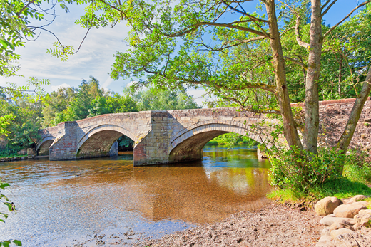
Pooley Bridge (Figure 10) was one of the worst affected bridges in the Cumbrian floods, scoring DL 4. This bridge was difficult to analyse directly with the restoration tasks (Table 1) laid out in the literature as no restoration task directly references a complete rebuild of a bridge, therefore a combination of information available was necessary. The temporary was assessed, not the permanent stainless steel bridge constructed nearly 6 years after the floods. While the new permanent bridge is significant in restoring the route to full capacity, it would be difficult to accurately analyse the complex restoration tasks completed, given the multiple years of planning, consultation and groundworks that took place during those 6 years (Snow and Tennant, 2022) including constructing a temporary pedestrian bridge while no vehicles could cross the river (Lytollis, 2019).
The temporary road bridge opened 106 days after the floods, on 20 March 2016, constructed directly on top of the location where the collapsed bridge once stood. This is quite a significant achievement as the closest restoration tasks to resemble what likely occurred (R1, R3 (×2), R12, R13, R20 and R23 (Table 1) have a mean time of 281.5 days (Table 5). This calculation assumed that the restoration works were fully sequential (i.e. no tasks were carried out in parallel). In practice, some tasks could be completed concurrently, which would reduce the overall restoration time. Therefore, it is important to consider a maximum duration of 442.5 days and a minimum duration of 121.3 days are included. This is coupled with the common census being that the idle time (time before any restoration works) is usually a minimum of 30 days for severely damaged bridges, as shown in Table 4. Therefore, the actual time it took to plan and construct the temporary Pooley Bridge (106 days) is significantly better than the estimated minimum time of 151.3 days that would have been predicted using the method of Mitoulis et al. (2021).
Restoration tasks for the temporary Pooley Bridge compared with data from Table 1
| Code | Duration: days | |||||
|---|---|---|---|---|---|---|
| Values from Table 1 | Temporary Pooley Bridge | |||||
| Min | Max | Mean | Min | Max | Mean | |
| R1 | 5.6 | 24.8 | 15.2 | 5.6 | 24.8 | 15.2 |
| R3 | 3 | 10 | 6.5 | 6 | 20 | 13 |
| R12 | 6 | 24.3 | 14.7 | 6 | 24.3 | 14.7 |
| R13 | 2.9 | 7.4 | 5.2 | 2.9 | 7.4 | 5.2 |
| R20 | 12 | 32 | 22 | 12 | 32 | 22 |
| R23 | 88.8 | 334 | 211.4 | 88.8 | 334 | 211.4 |
| Total | — | — | — | 121.3 | 442.5 | 281.5 |
This analysis does, however, have a significant flaw as there is no restoration task in Table 1 to represent replacing an entire bridge or installing a temporary bridge. Therefore, task R23 (demolition/replacement (part) of the bridge) was used as it was the closest resemblance to replacing the entire bridge, but with the high maximum (334.0 days), minimum (88.8 days) and mean (211.4 days) durations of this task, it does not accurately represent the reality of what occurred.
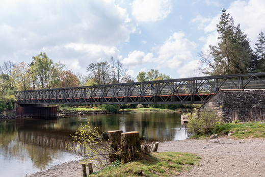
It was also assumed that the abutments were likely to have been mostly reused because the temporary bridge was in the same location as the former bridge. In addition, given that sources (BBC News, 2016) show that the largest damage occurred over the river itself, this likely helped reduce the reconstruction time significantly. New temporary cofferdams and the original stonework are shown in Figure 11, resulting in tasks R1 (armouring countermeasures and flow-altering/cofferdam) and R3 (temporary support of one abutment) being used. Therefore, emitting task R17 (reconstruction/replacement of the abutment and wingwalls) helped to reduce the reconstruction time significantly.
4.2 Establishing traffic capacity percentages
While educated assumptions were ultimately used for the traffic percentages in Table 2, as no paper sufficiently covers this area of restoration, reasons for the decisions made are now outlined.
In 2016, heavy goods vehicles (HGVs) comprised 16.9 billion vehicle miles out of the 327.9 billion total vehicle miles completed (approximately 5.2%) and buses comprised 2.6 billion vehicle miles (approximately 0.8%). Therefore, when weight limits are implemented, the traffic percentage must be at least 6% below 100%, if looking at the road types equally. However, a much greater effect is likely to be felt, given that the following additional factors must also be considered.
Buses are heavy transport vehicles that can carry much larger numbers of passengers than cars, with an estimated 11.4 passengers per bus in 2015/16 compared wit 1.55 passengers per car or van in 2016 (DfT, 2017a, 2023a).
In 2016 HGVs moved 1.89 billion tonnes of goods over 19.2 billion kilometres. This is something that must be factored in as they form the backbone of transporting goods such as food products throughout the UK (DfT, 2017b, 2023b).
The UK classes of roads (motorway, A roads, B roads, C roads and unclassified) have very different road usages. In 2016, 67.7 billion vehicle miles were completed on motorways, 144.9 billion vehicle miles were completed on A roads and 115.4 billion vehicle miles on the remaining B, C and unclassified roads (DfT, 2023b). This shows that a significantly high number of miles were completed on A roads, cementing their high importance in the UK. Although motorways have a lower number of miles completed on them, compared with A roads, they have higher speed limits and more lanes, which results in their significance being something not to be understated.
It can also be expected that heavier goods vehicles are more likely to use higher road classes. On a busy road (e.g. A or B road), one you would expect to see a higher frequency of HGVs, when compared with a quieter road (e.g. a C road or unclassified road). In the case of a bridge being imposed with a weight restriction, the busier route will likely be more affected by this restriction and therefore its capacity would be lower.
The percentages in Table 2 show a progressive decrease in capacity for motorways and other road types, with each road classification experiencing an estimated 5–15% reduction in capacity per category shift. This pattern reflects the greater impact of traffic control measures on higher capacity roads. The choice to adjust capacities in increments of 5% was made to simplify the implementation and future replication of these traffic models, ensuring ease of use and consistent applicability.
4.3 Bridge redesign issues
During restoration and reconstruction of the bridges in Cumbria, several key methodologies were employed to enhance resilience. One of the primary changes involved reducing or completely removing the number of piers located in riverbeds. This was done to minimise the risk of scour, which was a critical issue for many of the bridges during the floods. For instance, reductions can be seen in Pooley Bridge (2 to 0), Ford Bridge (2 to 0), Gowan Old Bridge (1 to 0) and Gooseholme footbridge (3 to 0). This was done to help remove potential future obstructions from the faster-flowing central sections of a river, which are more prone to damage, and mitigate the impact of future flooding. There are also reports that, as in the case of Backbarrow Bridge, some repairs from the 2009 floods potentially made the damage worse due to being made ‘taller and stronger’, which restricted river flow, applying high pressure on the bridges (The Mail, 2016).
Additionally, modern materials and construction techniques, such as the use of stainless steel in certain cases, were adopted to improve durability and reduce the likelihood of future damage. Pooley Bridge, Gowan Old Bridge, Hallbeck Bridge and Middleton Hall Bridge are all good examples of how changes were made to increase bridge resilience. Enhancing bridge resilience not only minimises future resource consumption, thereby boosting sustainability, but also reduces the likelihood of structural issues.
4.4 The priorities of CCC
With every bridge requiring its own carefully thought-out plan, CCC had to prioritise certain bridges to ensure that resources were being used effectively.
According to the data shown in Figure 3, CCC’s main priority was to reopen bridges on the busier A and B roads, given their high importance to the local area. This also aligns with the priorities set out in the impact assessment (CCC, 2018a).
Many bridges were reopened by CCC once temporary measures were implemented, such as Victoria Bridge and Ford Bridge (CCC, 2016c, 2016d), with these bridges opened before all structural repairs were completed. This implies that, while the bridges were not structurally reinstated back to pre-flood levels, they were still considered safe to open to some degree of capacity, with the added benefit of also helping increase the total capacity of the entire Cumbrian road network.
Pressure from local stakeholders, such as residents and local businesses, may have played a key part in opening the bridges as quickly as possible, despite bridges not being fully structurally reinstated.
5. Analysis of findings
The results from applying the traffic reinstatement model to the 2015 Cumbria floods case study show how effectively the region’s bridges were restored after the 2015 floods. The model provides a clear indication of how a set of bridges recovered in terms of traffic capacity and the time taken to fully reinstate road access.
However, several limitations were noted during the analysis. First, the availability of detailed inspection data for each bridge was limited, leading to a reliance on generalised restoration models. Additionally, the traffic reinstatement model assumes sequential restoration work whereas, in reality, multiple repairs could be conducted in parallel, potentially altering the estimated recovery times.
Despite these limitations, the model offers valuable insights into the resilience of bridge infrastructure in flood-prone regions. It also highlights the importance of detailed inspections, such as those requiring dive crews, that revealed hidden damage, emphasising the need for thorough post-disaster assessments.
The final flood risk management strategy set out CCC demonstrates that Cumbria is now better prepared than in 2015 (CCC, 2022b). Measures such as improving the resilience of critical infrastructure and updating emergency response protocols suggest that Cumbria is now better equipped to handle similar future events.
6. Conclusion
Restoration models for bridges damaged during the 2015 Cumbria floods have been presented. The restoration analysis revealed that severely damaged bridges (DL 4) had a mean restoration time of 11 months, with most priority bridges on A roads being restored within 6 months. Restoration projects, such as Pooley Bridge's rapid 106-day reopening of its temporary bridge, achieved exceptional results with a 45% reduction in estimated timelines by employing concurrent tasks. Key lessons show that implementing scour protection and reducing in-water piers significantly improved resilience, streamlining future restoration needs.
The methodologies applied here can be used for future disaster recovery planning, offering a framework for evaluating bridge resilience and restoration efforts. This model can also be adapted for use in different regions and disaster types, allowing policymakers and engineers to prioritise infrastructure recovery based on real-time assessments.
Future work could focus on refining the models by incorporating more advanced techniques, such as real-time monitoring of bridge conditions during floods, and integrating machine learning to predict recovery timelines more accurately. Expanding the dataset to include other types of infrastructure affected by floods would also enhance the applicability of the models developed in this study. Additionally, further research could be used to assess different aspects such as the socio-economic impact of bridge closures on communities during extended restoration periods. One key limitation of this study is the assumption that all restoration activities occur sequentially, which may not fully reflect real-world conditions where multiple tasks can be conducted in parallel. Additionally, the availability of detailed damage data varied across bridges, affecting the granularity of some analyses.
Acknowledgments
Dr Mitoulis would like to acknowledge funding by the UK Research and Innovation (UKRI) under the UK government’s Horizon Europe funding guarantee [grant agreement No: 101086413, EP/Y003586/1, EP/Y00986X/1, EP/X037665/1]. This is the funding guarantee for the European Union HORIZON-MSCA-2021-SE-01 [grant agreement No: 101086413] ReCharged – Climate-aware Resilience for Sustainable Critical and interdependent Infrastructure Systems enhanced by emerging Digital Technologies.


