A 190 m long flume for investigation of debris flow impacts on multiple flexible barriers

$Cc$

coefficient of curvature of soil

$Cu$

coefficient of uniformity of soil

$D50$

particle diameter where 50% of sample mass is smaller than that sieve size

$Fdynamic$

hydrodynamic impact force exerted by debris flow on a barrier

$Fimpact$

total impact force exerted by debris flow on a barrier

$Fstatic$

hydrostatic impact force exerted by debris flow on a barrier

$Fr$

Froude number

$g$

acceleration due to gravity

$H$

barrier height

$h$

flow height

$k$

static impact coefficient

$L$

overflow handing distance

$uw$

pore water pressure

$v/vavg$

flow velocity/ average flow velocity

$vof$

overflow velocity

$w$

channel/flume width

$α$

dynamic impact coefficient

$θ$

slope angle

$θ0$

overflow launch angle

$ρ$

bulk density of debris mixture

$σn$

basal normal stress

Debris flows exhibit scale dependency due to complex interactions between solid and fluid phases (Iverson, 1997). In small-scale experiments, fluid viscosity may significantly influence debris flow behaviour, whereas in real-world scenarios, Coulomb friction often predominates with evolving pore water pressure (Iverson et al., 2011). Moreover, pore water pressure dissipation occurs more rapidly in small-scale experiments than in field conditions due to the shorter drainage path along the flow depth (Iverson, 2015). While field data can provide insights into debris flow mechanisms (McArdell et al., 2007; Zhou & Ng, 2010), the complexity and heterogeneity of materials and natural settings pose challenges for reproducibility and theoretical comparison (Choi et al., 2024). Consequently, large-scale physical modelling serves as a systematic tool for generating reproducible experimental data not only for elucidating debris flow mobility but also its interaction with mitigation measures.

In recent years, flexible barriers have been increasingly adopted as a replacement or in combination with rigid reinforced concrete barriers for mitigating debris flow hazards in mountainous torrents (Berger et al., 2021). Flexible barriers are lightweight, more easily installed in complex terrains without heavy foundations and blend with their surroundings, offering a cost-effective, environmentally friendly and low carbon-dioxide solution. Structurally, the deformability of flexible barriers prolongs impact duration, thereby reducing the force exerted compared to rigid barriers (Zhan et al., 2019; Ng et al., 2020b). For mitigating large volumes of debris, multiple flexible barriers are advantageous over a single rigid barrier due to progressive debris retention, minimising flow acceleration and enhancing energy dissipation (Wendeler et al., 2008). This allows for smaller barrier sizes with reduced construction costs and time. Despite their technical value, there is still a need for research into scientifically sound designs for single and multiple flexible barriers due to the challenge of rationally scaling debris flows (Choi et al., 2024).

Numerous studies have explored the impact mechanisms of debris flow against flexible barriers across various scales. Bugnion et al. (2012) and Wendeler (2016) studied impacts on flexible debris flow and shallow landslide barriers installed in a quarry and in a mountain torrent. These tests were limited to a barrier at a time and repeatability was limited due to large installation works. Flume tests with clear boundary conditions support a better understanding of variables in the flow and barrier set-up. Small-scale laboratory flume experiments have examined the impact mechanisms of dry granular flow (Ashwood & Hungr, 2016), slurry (Speerli et al., 2010) and debris flow (Song et al., 2022) against flexible barriers. However, these experiments often feature significantly smaller flow heights than those in field conditions, resulting in incorrect stress conditions and lower impact energy. In addition, small-scale flumes, typically up to 0·3 m wide, model flow–barrier interaction with a plane strain assumption. This set-up constrains the barrier’s deformation along its span, leading to incorrect stiffness (Wendeler & Volkwein, 2015). As the dynamics of debris flow–barrier interaction are governed by barrier stiffness, wider flumes are necessary to model the three-dimensional (3D) deformation of flexible barriers reliably. Some studies have attempted to address this limitation by installing a wider span of flexible barriers at the channel’s end (DeNatale et al., 1999), but this set-up limits testing to one barrier at a time. Consequently, research has primarily focused on debris flow impact against a single flexible barrier (Bugnion et al., 2012; Wendeler, 2016; Tan et al., 2020). Only a couple of studies have investigated multiple flexible barriers’ efficacy in resisting debris flows (Speerli et al., 2010; Ng et al., 2023). A systematic study of the impact of debris flow on multiple flexible barriers requires a flume sufficiently wide to model 3D deformations and long enough to accommodate multiple barriers.

Recent debris flow tests on a natural hillslope catchment with an 800 m channel length and 446 m³ debris volume (Yune et al., 2023) provide valuable data on debris flow dynamics. However, unique and dynamically changing boundary conditions, due to erosion and deposition, complicate interpretation of the results (Iverson, 2015), especially for flow–barrier interaction. Advances in large-scale flume facilities aim to minimise scale effects in modelling debris flow and flexible barrier interactions (Ng et al., 2020a) while allowing rigorous control of test variables to investigate critical design conditions. Ng et al. (2020a) summarised test results from various scales and proposed an equation for estimating debris flow impact force (F_impact) on a single flexible barrier, expressed as follows:

where F_dynamic is the dynamic force; F_static is the static force; α and k are dynamic and static impact coefficients, suggested as 1·0 for flexible barriers;$ρ$ is the bulk density; w is the flow width;$v$ and $h$ are flow velocity and height before impact;$g$ is the gravitational acceleration. Equation (1), with recommended coefficients, has only been validated for debris flows up to 9 m³ (Ng et al., 2020a), much less than typical debris flow volumes observed in the field (Cui et al., 2005; Kwan, 2012). Multiple barrier design also requires the evaluation of debris overflow and landing for optimal barrier spacing. Kwan et al. (2015) multiple barrier framework has been updated to improve debris flow landing distance predictions with varying solid fractions (Ng et al., 2024c), clay contents and launch angles (Ng et al., 2024a). Ng et al. (2024a) also proposed a new analytical equation for overflow landing distance, which is expressed as follows:

where L is the overflow landing distance; H is barrier height;$vof$ is overflow velocity; $θ$ is slope inclination; and$θ0$ is the overflow launch angle. With horizontal overflow velocity (that is$θ0=0°)$ and a vertical barrier face, equation (2) reduced to the original equation proposed by Kwan et al. (2015). A numerical parametric study by Ng et al. (2024b) identified optimal spacing between barriers at L/H = 2·0, minimising downstream impact force. This spacing prevents debris flow acceleration and avoids direct airborne debris impact. Although equation (2) has been verified for dual barriers with flow volumes up to 9 m³, shorter lengths of existing flume facilities preclude modelling three or more barriers in series. Thus, further investigation of debris flow–multiple barrier interactions with larger flow volumes in a long flume is crucial for advancing multiple flexible barrier design.

This study investigates debris flow impact dynamics against four flexible barriers using a newly developed 190 m long, 6 m wide flume facility with 180 m³ of flow material. First, the unique features and capabilities of the new flume, alongside sensors and instrumentation, are introduced. Then, the existing design criteria proposed by Ng et al. (2020a, 2024a) are validated through new test results of debris flow impact and overflow against multiple flexible barriers. Finally, the results and implications for future research are discussed.

The Hong Kong University of Science and Technology (HKUST), in collaboration with the Institute of Mountain Hazards and the Environment (IMHE) of the Chinese Academy of Sciences (CAS) and Huadong Engineering Corporation Limited (HEDC), has constructed the world’s largest flume facility at the Dongchuan Debris Flow Observation and Research Station (DDFORS) in Kunming, Yunnan, China. Fig. S1, in the online supplementary material, shows the newly established flume facility located at 26°14’47” N and 103°08’06” E, at an elevation of approximately 1500 m (Ng et al., 2025).

The 190 m long flume, constructed from reinforced concrete, features a rectangular cross-section measuring 6 m wide and 4 m high, making it the largest of its kind in the world. Its design allows for well-controlled and specifiable boundary conditions, facilitating reproducible debris flow impact experiments and providing reliable data for numerical model validation. This is crucial not only for elucidating debris flow dynamics and flow–barrier interaction but also for developing guidelines for debris-resisting barrier design, where test repeatability and knowledge of boundary condition are essential for interpreting debris flow impact mechanisms.

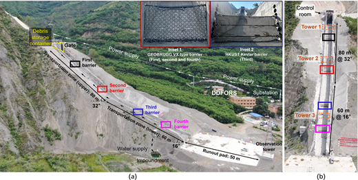
Figure 1(a) shows the aerial side view of the newly established flume, which includes a 16 m long storage container with a maximum capacity of 500 m³ highlighted in yellow, featuring a 13° inclined base equipped with a water supply system for saturating the debris solid fraction. An electro-hydraulically controlled, cable-operated gate at the downstream end initiates a dam-break flow. The flume’s 140 m transportation zone is divided into two sections: the upper section, 80 m long, is inclined at 32°, while the lower section, 60 m long, is inclined at 16°. The lower section transitions to a 50 m horizontal runout pad, monitored by an observation tower with cameras. Flexible barrier locations are highlighted in black, red, blue and pink, respectively, for the first, second, third and fourth barrier. Ground anchors are installed at these locations to allow barrier installation without posts. The height of the side walls is increased to 5 m at these sections to prevent lateral overflow. Inset 1 shows the modified Geobrugg VX type barrier, while inset 2 shows the HKUST Kevlar flexible barriers used in this study.

Figure 1(b) shows the front elevation view of the flume. A control room beside the storage container manages gate operation, data logging from multiple sensors, and high-speed camera recording. Towers, measuring 6 m high and spanning 7 m across the flume width, facilitate sensor and camera installation above the first, second and fourth barrier locations. Towers 1 and 2 are located 20 m and 55 m from the gate, respectively, in the upper section, while tower 3 is located 120 m from the gate in the lower section. A detailed layout of different types of sensors and instrumentation installed along the transportation zone to monitor the test is provided in the online supplementary material (Figs S2, S3 and S4) (Ng et al., 2025). Table S1 summarises the sensors and instrumentation utilised in the 190 m long flume.

The debris material for the flume experiments is sourced from sediments deposited by debris flows in the Jiangjia ravine (Cui et al., 2005; Hu et al., 2011). Debris material with a maximum particle size of 200 mm is used in this study. Using the unified soil classification system (ASTM, 2017), the debris material can be classified as well-graded gravel with sand. The material has a coefficient of uniformity$Cu$ of 55·4 (⁠$Cu$ > 4·0) and a coefficient of curvature$Cc$ of 1·1 (⁠$1·0≤Cc≤3·0)$⁠. Over 15% of the material is sand, with a characteristic grain size (D₅₀) of 20 mm. Details of particle size distribution (PSD) analysis, and the preparation of debris material are provided in the online supplementary material, Fig. S5. In this study, 180 m³ of debris mixture was prepared, comprising 40% solids and 60% water by volume with a design density of 1600 kg/m³.

Four flexible barriers were used in this study to investigate debris flow–multiple flexible barrier interactions. Flexible barriers made of two different types of materials were used in this test: a steel ring net barrier and a Kevlar flexible barrier. The steel ring net barrier is a modified Geobrugg VX type flexible barrier (see Fig. 1(a), inset 1), while the Kevlar flexible barrier was newly developed in-house at HKUST (see Fig. 1(a), inset 2). The steel ring net barrier was designed as the first (FB1), second (FB2) and fourth (FB4) barriers, whereas the Kevlar flexible barrier was used as the third (FB3) barrier. Fig. S6 in the online supplementary material (Ng et al., 2025) shows the detailed design drawings of both types of flexible barriers.

After installing the barriers in the flume, preparing debris material in the storage container and connecting all the sensors and instrumentation to the datalogging system, the test was executed. Unmanned aerial vehicles (UAVs) were flown to their respective positions to capture the flow kinematics. The action cameras and high-speed cameras that were strategically placed along the flume were triggered to start recording. The datalogger was simultaneously triggered as the electrical switch was turned on to open the gate. The hydraulic pins restraining the gate were released and the cable winch swung the door open, initiating a dam-break of debris material. This paper reports the result from one test using 180 m³ volume of debris making impact against four flexible barriers.

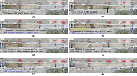
Figure 2 shows the overall kinematics of debris flow in the 190 m long flume, captured by an UAV, depicting the key stages in chronological order (see online supplementary material, video V1-UAV.mp4) (Ng et al., 2025). The timeline begins at t = 0 s, marking the start of the gate opening and recording by the data logger. At t = 37 s (Fig. 2(a)), the granular debris front reaches the first barrier (FB1), while muddy water passes through, reaching basal cell C4. FB1 intercepts the debris flow front, undergoing noticeable deformation by t = 40 s (Fig. 2(b)). Concurrently, the muddy water reaches the second barrier (FB2). As the flow impacts FB1, debris runs up and rolls back upstream (t = 46 s, Fig. 2(c)), with partial discharge through the mesh. By t = 49 s, debris exhibits a peak run-up height, overtopping FB1 (Fig. 2(d)), although much material is retained. At this point, muddy water reaches the third barrier (FB3). The overflow continues atop FB1 at t = 59 s (Fig. 2(e)), with granular debris material reaching FB2. By t = 67 s (Fig. 2(f)), debris flow impacts and partially discharges through FB2 and FB3, while muddy water reaches the fourth barrier (FB4). Due to limited overflow and discharge of muddy water and fines at FB1, downstream barriers remain unfilled. Overflow occurred only at the first barrier. Debris overflow ceases at t = 101 s (Fig. 2(g)), with only muddy water discharging through the mesh. By t = 166 s (Fig. 2(h)), the impact ends with debris deposited behind the barriers with FB1 filled to the crest and the remaining barriers retaining a negligible amount of material. Quantitative assessment of debris retention behind each barrier is provided in a later section. In addition to the UAV footage, videos captured by high-speed cameras and DJI action cameras are used to deduce flow velocity and Froude number at each barrier location.

A detailed description of the kinematics at each of the four flexible barriers during key instances of debris flow impact is provided in the online supplementary material, Figs S7–S10. Corresponding videos captured by the respective DJI action cameras at each barrier are also provided in the online supplementary material. The observed kinematics, combined with sensor data, are used to elucidate the effects of multiple barriers on debris flow properties in the next section.

Debris flow properties measured by multiple sensors and instrumentation are used in characterising the flow regime at each barrier location. Debris flow height, flow velocity, impact pressure, basal normal stresses and pore pressures are the key physical properties of debris flow measured in this study to elucidate the impact and overflow mechanism, and to calculate the design impact force on a flexible barrier.

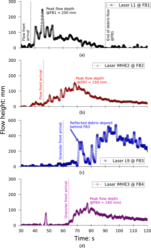
Flow height is captured by the laser sensors installed on the monitoring towers adjacent to the flexible barriers (see Fig. S3). Fig. 3(a) shows the time histories of debris flow height measured by different laser sensors in front of the different flexible barriers. For clarity of presentation, flow height measurement from only one laser sensor in front of each flexible barrier is shown. Flow heights measured by all the sensors at respective barrier locations along the flume reveal largely uniform flows (see Fig. S11 in the online supplementary material) (Ng et al., 2025). The flow front reaching the first barrier is slightly non-uniform, immediately followed by a uniform flow body. Fig. 3(c) shows the flow height in front of the first flexible barrier FB1 (at basal instrumentation cell C1), measured by the laser sensor L1. The sensor L1 is located 7 m upstream of FB1 (see Fig. S2). The initial granular debris flow front arrives at t = 37 s. The granular debris flow head immediately follows the flow front, measuring 150 mm high at t = 40 s. The thickest part of the debris flow body arrives at t = 46 s, which measures around 250 mm. The flow height time history reveals that the debris flow passes through the monitoring section in pulses, with flow height of around 150 mm until t = 55 s. The measured pulses in the flow height corroborate well with the observed waves on the debris flow surface in the captured video footage. Thereafter, the debris flow height progressively recedes until t = 90 s, when all the debris material has been released from the storage tank. Since the laser sensor L1 does not measure the height of debris deposited behind the barrier FB1, the measured flow depth at the end of the test reaches zero.

Figure 3(b) shows flow height in front of FB2 (at C4) measured by sensor IMHE2 located in the middle. Unlike L1, sensor IMHE2 shows a gradual increase until t = 47 s, due to limited discharge through FB1. Debris overflows FB1 after t = 49 s (see Fig. 2(d)), mixes with debris discharged through the mesh, and peaks to 150 mm at t = 68 s. Debris retention at FB1 reduces the flow height reaching FB2 after t = 75 s. Although muddy water overflows FB1 until t = 101 s (see Fig. 2(g)), granular debris overflow ceases at t = 80 s. Continuous muddy water discharge results in a 30 mm height at FB2, even after t = 101 s. Sensor IMHE2, like L1, does not measure the tail end of debris deposited behind FB2.

Figure 3(c) illustrates flow height in front of FB3 (at C6), with the y-axis ranging from 0 to 600 mm, twice that of Figs 3(a), 3(b) and 3(d). The ordinate is scaled to accommodate the peak deposition height behind FB3 captured by sensor L9, unlike at FB1 and FB2 where the tail end of the deposited debris is not captured by laser sensors. Despite UAV-captured flow kinematics showing muddy water reaching FB3 at t = 49 s, significant increase in flow height is not measured until t = 60 s. The measured flow height is 80 mm at t = 67 s when granular debris reaches and accumulates behind FB3 (see Fig. 2(f)). This reduced flow height is due to limited discharge through FB2. The pulse at t = 70 s corresponds to sloshing of deposited debris. As overflow from FB1 passes FB2 and reaches FB3, deposition behind FB3 enlarges considerably. At t = 98 s, the sensor L9 captures the peak deposition height of 550 mm. After t = 100 s, debris arrival at FB3 reduces, and discharge through FB3 continues, progressively reducing deposit height beyond t = 120 s.

Figure 3(d) shows flow height in front of the fourth barrier FB4 measured by sensor IMHE3, exhibiting a trend similar to FB1 (Fig. 3(a)) and FB2 (Fig. 3(b)). The flow front of muddy water reaches FB4 at t = 59 s (see Fig. 2(e)). Flow height starts to increase at t = 64 s upon the arrival of granular material, peaking at 140 mm at t = 78 s. The 16° flume inclination between FB3 and FB4 decelerates the flow, increasing flow height. Limited debris is deposited behind FB4, and sensor IMHE3 does not measure the height of deposited debris. As debris discharges past FB4 by way of basal discharge, the flow height recedes after t = 80 s since only muddy water arrives after granular materials have been retained at the three upstream barriers.

The measured time histories of flow height in front of different barriers show a significant drop in flow height due to interception of debris flow by upstream barriers. Limited overflow and partial discharge of fines filtering through barrier mesh result in a prolonged debris flow surge with reduced flow height at downstream locations (exceeding$Δt≈$ 60 s). In contrast, debris flow surge at FB1 lasts for a shorter duration (around$Δt≈$ 40 s) yet with a greater flow height. These flow heights are used to estimate the Froude number and impact pressures at each barrier, and to evaluate basal normal stresses and pore pressures at different instrumentation cells, elucidating debris flow dynamics.

Froude number (⁠$Fr$⁠) is defined for gravity-driven free surface flows as the ratio of inertial stress to gravitational stress (Iverson, 2015), which is expressed as follows:

where$v$ is the flow velocity;$g$ is the acceleration due to gravity;$h$ is the flow height; and$θ$ is the slope inclination. Froude number is used to characterise the flow regimes by assessing whether it is inertia dominated (⁠$Fr > 1$⁠; supercritical) or gravity dominated (⁠$Fr < 1$⁠; subcritical). In addition,$Fr$ is one of the key variables governing debris flow impact mechanisms and induced impact forces on barriers (Hübl et al., 2009; Hu et al., 2011).

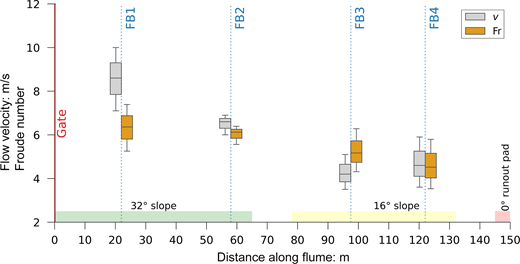
Figure 4 illustrates the variation of debris flow velocity and Froude number at four barrier locations. The gate serves as the origin for measuring distance along the flume, with barriers located at 22·0 m (FB1), 58·0 m (FB2), 97·5 m (FB3) and 122 m (FB4) from the gate. The flow velocity distribution at each barrier is shown in a grey boxplot with whiskers. Flow velocity is deduced from multiple cameras. The observed debris flow surge fronts were manually tracked over specified distances to obtain the flow velocities (see Figs S12 and S13 in the online supplementary material for details) (Ng et al., 2025). The average flow velocity values are plotted at each barrier location with the range of minimum and maximum values shown by the whiskers. The average flow velocity (⁠$v$⁠) is used to estimate impact pressure. Flow velocity is highest at FB1 (8·6 m/s) and reduces to 6·6 m/s at FB2 and 4·2 m/s at FB3, as a large quantity of debris is intercepted by FB1. The discharge velocity past FB1 is lower due to momentum transfer during flow–barrier interaction. The flume inclination changes from 32° to 16° at FB3, further reducing the velocity as the component of gravity driving the flow reduces. However, velocity increases slightly at FB4 to 4·6 m/s, which can be attributed to acceleration of largely muddy debris flowing unimpeded past FB3 on a uniform slope.

The$Fr$ variation at each barrier location is shown in an orange boxplot with whiskers, calculated using peak flow heights from laser sensors (Figs 3(a)−3(c)). The$Fr$ is highest at FB1 (6·4), with a corresponding peak flow height of 250 mm. After debris interception at FB1, peak flow height reduces to 140 mm at FB2 and 70 mm at FB3, resulting in$Fr$ of 6·1 and 5·2, respectively. Despite slightly increased velocity at FB4, flow height increases more pronouncedly due to basal resistance from the flatter bed, reducing the$Fr$ to 4·5. The modelled flow exhibits$Fr$ similarly to natural debris flows in steep terrain (Hübl et al., 2009), highlighting its geomorphological relevance in investigating debris flow dynamics and debris flow–barrier interactions.

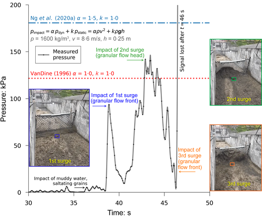
Figure 5 shows the time history of measured impact pressure by a pressure plate (Fig. S4c in the online supplementary material) with key instances shown in accompanying inset images. At t = 36 s, the plate registers a peak impact pressure of 5 kPa as muddy water and saltating grains hit the plate. At t = 38 s, the granular debris front exerts another peak impact pressure of 90 kPa, corresponding to the first surge. A temporary drop in the impact pressure, caused by the second surge flowing sidewards in the flume and missing the plate, occurs until t = 40 s. The pressure increases again after t = 41 s when the second surge spans the flume width, peaking at 149 kPa at t = 43 s. By t = 44 s, the plate is fully submerged by debris. The third surge overrides the submerged plate, causing signal loss after t = 46 s. For this reason, only pressure measured up to t = 46 s is used for interpretation. Measured pressures are compared with analytically estimated pressures using design flow density (1600 kg/m³), peak velocity (8·6 m/s) and flow height (250 mm) at the plate location. The reference line by VanDine (1996) under-predicts peak impact force on rigid barriers (α = 1·0, k = 1·0). The recommended pressure coefficients (α = 1·5, k = 1·0) from Ng et al. (2020a) provide a conservative upper bound for the measured impact pressures from the first two surges of incoming flow. However, it is acknowledged that the signal was lost immediately after the third surge, which poses a significant challenge in comprehensively validating the existing design criterion for the entire time history.

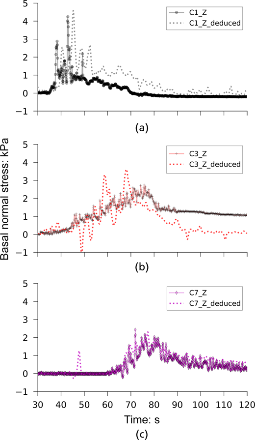
Figures 6(a)–6(c) present time histories of measured basal normal stress at cells C1, C3 and C7 along the flume (see online supplementary material, Fig. S2). These cells are chosen to specifically represent debris flow properties before impacting a barrier (C1), immediately after the landing of overflow (C3) and after filtering past the barrier without overflow (C7), respectively. In addition, basal normal stress calculated from measured flow height and design density (1600 kg/m³) at the respective basal cell location is shown. Comparison of measured and deduced results shows reasonable agreement across different cells, albeit with deduced values slightly higher than the measured ones. This discrepancy may be attributed to a lower density of the bulk debris mixture due to flow thinning as well as a non-uniform solid fraction, unlike that assumed in the designed mixture. In Fig. 6(a), the flow front reaches cell C1 at t = 37 s, resulting in a rapid increase in basal normal stress. The arrival time aligns with flow height measurements (see Fig. 3(a)). Debris flow arrives in surges, causing fluctuations in normal stress between t = 40 s and t = 80 s. Similar observations have been reported by Aaron et al. (2025) using high-resolution field measurements, highlighting the severe implications of surge waves in relation to debris flow hazards. They revealed that surge waves can magnify peak discharge by two to three times, greatly enhancing flow height and velocity, which can significantly increase the impact force on a barrier. In this study, the first surge exerts 2·6 kPa normal stress at t = 40 s. At t = 44 s, the debris flow head overrides cell C1, with normal stress reaching 3·9 kPa. As the flow body passes from t = 45 s to 60 s, progressive thinning reduces the stress from 1·2 to 0·5 kPa. Continued discharge of watery debris past cell C1 occurs until t = 90 s, with stress reducing to zero thereafter. Deduced stress from flow height shows a 1·0 s delay in peak stresses due to the orientation of laser sensor L1 downstream of cell C1.

Similarly, Fig. 6(b) shows basal normal stress history at cell C3, which rises after t = 40 s with debris discharge past FB1. FB1 intercepts the flow, initially allowing limited debris to pass through, slowly ramping up stress in C3 until t = 50 s. As debris overflows FB1, discharge over C3 increases, raising the normal stress until t = 75 s. Thereafter, overflow reduces until it ceases at t = 101 s, with only muddy water filtering through FB1’s mesh. This transition marks a sharp stress drop at t = 80 s. Continuous discharge through the mesh of FB1 causes a progressive stress decrease from t = 80 s onwards. Basal normal stress calculated from flow height captures the trend but shows multiple surge fronts, evident in the captured kinematics as flow approaches FB2 (see Fig. 2(e)).

Figure 6(c) shows basal normal stress history for cell C7, upstream from FB4. Despite debris retained at FB2 and FB3, basal discharge results in stresses similarly to C3 (around 2 kPa). The flow front arrival, peak normal stress and attenuation to zero are evident in C7. Calculated basal normal stress shows reasonable agreement with measured values. Basal cells reliably capture flow basal stresses, reflecting flow behaviour changes due to the progressive retention of debris in multiple barriers. Analysis of measured results show that basal normal stress data enable first-order estimation of debris flow bulk density when coupled with flow height measurements.

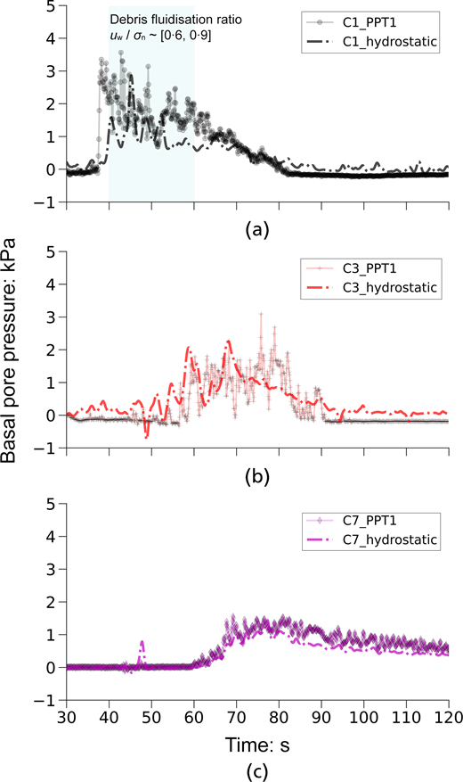
Figure 7 shows time series of basal pore pressure measured at cells C1, C3 and C7 by pressure transducers located on the upstream edge (PPT1) of each cell (see online supplementary material, Fig. S4b). Each basal pore pressure sensor is equipped with a stainless steel filter element with 1 mm wide opening. The filter element is a 60 mm square and 3 mm thick plate with a 20 mm dia. laser cut mesh at its centre. Once installed, the filter element sits flush with the top sensing plate in a recessed slot to prevent flow separation and avoid spurious pressure readings. Fawley et al. (2025) have recently reported similar findings regarding the effects of recessed and elevated filters on spurious pore pressure readings while investigating idealised two-phase mixtures of water and ceramic grains.

Figure 7(a) shows measurements from transducer C1_PPT1, indicating debris flow front arrival at cell C1 at t = 37 s. As the granular debris front flows over C1_PPT1, basal fluid pressure rapidly increases to 3·2 kPa. The thickest part of the flow arrives at t = 44 s, exhibiting another pressure pulse of 3·6 kPa. Continuous flow overrides cell C1, with surges reflected in the pore pressure evolution. Comparing the pore pressure history (Fig. 7(a)) with basal normal stress (Fig. 6(a)) at C1 reveals fluidisation, inferred from the pore pressure to normal stress ratio (that is fluidisation ratio =$uw/σn$⁠), fluctuating between 0·6 and 0·9 from t = 40 s to 60 s (shaded region). Hydrostatic pore pressure calculated through measured flow height at C1 using density of 1000 kg/m³ for water shows reasonable agreement with measured results, albeit with a slight delay. Dynamic pore pressure exceeds deduced values by 1·2 to 1·8 times between t = 40 s and 60 s, which is likely to be due to the use of water as pore fluid, neglecting suspended fines’ contribution to fluid density (Iverson, 1997). As debris flow recedes, pore pressure at C1 decays to zero between t = 70 s and 90 s.

Figure 7(b) shows basal pore pressure evolution at cell C3, which exhibits a delayed response until t = 50 s as FB1 retards flow through the mesh. Rapid pressure increase occurs from t = 50 s to 70 s, corresponding to increased discharge from overflow. From t = 70 s to 90 s, pore pressure at C3 decreases as debris flow recedes. Pore pressure reduces sharply from 1·5 kPa at t = 80 s to zero by t = 90 s. Compared to Fig. 7(a), which shows a characteristic evolution of pore water pressure in unimpeded flows, Fig. 7(b) reveals how flow–barrier interaction changes debris flow dynamics downstream of the barrier. Debris flow interception and overflow not only reduce the peak pressure but also extend the time to reach the peak. Thereafter, a rapid drop in pore pressure is observed as debris retention in the upstream barrier leads to cessation of debris flow downstream.

Figure 7(c) illustrates pore pressure evolution at cell C7, aligning with measured basal normal stress in Fig. 6(c) between t = 50 s and 80 s. Basal normal stress decreases from 1·6 kPa at t = 80 s to 1·0 kPa at t = 120 s. Deduced pore pressure from flow height measurement shows better agreement with pore pressure than normal stress in overall trend. Measured basal normal stress (Figs 6(a)–6(c)) and pore pressures (Figs 7(a)–7(c)) characterise the state of stress in debris material (fluidisation ratio) and help in the assessment of flow mobility. Differences in normal stress and pore pressure evolution at various locations along the flume reflect how barriers can significantly affect debris flow dynamics in the downstream sections.

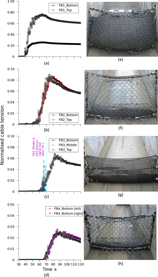
Figures 8(a)–8(d) display the measured time histories of normalised cable tension in the horizontal supporting cables of four flexible barriers, while Figs 8(e)–8(h) show images of these barriers at the end of the test. The measured cable tension is normalised by the minimum breaking load of a Geobinex 22 mm steel rope (400 kN). Fig. 8(a) illustrates cable tension in the top and bottom cables of the first barrier (FB1). The X-axis represents elapsed time from gate opening, ranging from t = 30 s to t = 120 s. FB1 is supported by two horizontal supporting cables: the top cable (FB1_Top) and the bottom cable (FB1_Bottom). The debris flow front reaches FB1 at t = 37 s (see online supplementary material, Fig. S7a), exerting an initial normalised force of 0·15 on the top cable and 0·05 on the bottom cable. After t = 40 s, normalised top cable tension increases in surges, peaking to 0·76 at t = 63·5 s, while the bottom cable tension peaks to 0·26 at t = 63·4 s. The peak dynamic impact force on FB1 occurs during continuous debris overflow (see Figs 2(e) and S7e). Tension in the top cable is three times greater than in the bottom cable, which is attributed to its deflection during impact (see Fig. 2(c)), the weight of debris retained by the mesh and the lateral pressure of retained debris. Most debris material is retained at FB1, resulting in limited downstream discharge of predominantly finer material filtered through the barrier mesh. Consequently, peak impact forces on the second, third and fourth barriers are about one-tenth of those on FB1. Fig. 8(b) shows peak normalised tension of 0·085 in both supporting cables of FB2. Similar results are observed for FB3 (Fig. 8(c)) with a peak normalised tension of 0·068 in the top cable. Unfortunately, signals for middle and bottom cables were lost after t = 70 s. Fig. 8(d) shows FB4 with peak normalised tension around 0·028 in bottom horizontal supporting cable. Without overflow, FB2, FB3 and FB4 exhibit peak forces corresponding to peak flow height measured at these barriers (see Figs 3(a)–3(c)). A clear trend of reduced peak impact force across downstream barriers is observed as debris is progressively intercepted and retained upstream. Figs 8(e)–8(h) illustrate a decrease in debris volume retained behind each barrier along the slope, which is discussed later.

Cable tension forces are resolved into barrier impact forces using the deformed configuration suggested by Song et al. (2018). The calculated peak impact force at FB1 is 170 kN, considering a 12° deflection angle of the top cable. Design impact force is estimated using equation (1), with a flow velocity of 8·6 m/s, flow depth of 0·25 m and design density of 1600 kg/m³. Pressure coefficients α = 1·0 and k = 1·0, as recommended by Ng et al. (2020a), result in a design impact force of 173 kN, validating the design criteria’s estimation of impact force on flexible barriers.

Debris overflow and landing occurred solely at the first barrier (FB1) during this test, fully utilising its retention capacity (see online supplementary material, Fig. S7f) (Ng et al., 2025). The debris retention at FB1 significantly reduced downstream debris flow discharge. Consequently, the remaining barriers were only partially filled from debris passing through the upstream barrier mesh. UAV-captured kinematics in Fig. 2 show overflow commencing at t = 49 s and continuing until t = 101 s. Overflow occurred only after the FB1 was filled to the crest.

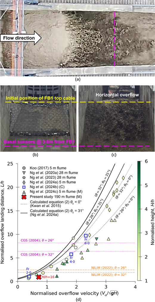
Figures 9(a)−9(c) show the top plan and front elevation views of debris overflow at the first barrier. Overflow launches horizontally from the barrier crest, landing downstream on the flume. Landing distance ranges from 2·7 m to 3·8 m from the barrier line, attributed to turbulent overflowing debris. The dashed pink lines in Figs 9(a) and 9(b) mark the basal instrumentation cell C2, located 3·8 m downstream. As overflow progresses, velocity peaks and then reduces to zero, mirroring landing distance trends. Maximum overflow velocity ranges from 3·0 m/s to 4·5 m/s, corresponding to maximum landing distance captured in flow kinematics.

Figure 9(d) shows normalised overflow landing distance (L/H) against normalised overflow velocity$vof/gH$ for varying barrier-to-flow height (H/h) ratio based on equation (2). The first barrier is installed on a 32° incline. The measured L/H in this study is 0·94, with a normalised overflow velocity of 0·72 (red X marker). Measured (M) and computed (C) results aggregated from existing studies are compared across a wide range of$Fr$ from 1·0 to 8·0. By comparing equations (2) and (3),$Fr$ can be used as a proxy for the normalised overflow velocity. The colour map of filled markers for these existing studies represent the H/h ranging between 1 and 6. Most 5 m flume tests were conducted at an inclination (⁠$θ$⁠) of 26° and 32° while the 28 m flume tests were conducted at 20°. Koo (2017) varied the first barrier height in a 5 m flume, maintaining constant flow$Fr$ to study the effects of barrier height on landing distance. Complementarily, Ng et al. (2024b) maintained a constant H/h of 2·0 while varying$Fr$ from 2 to 6 to evaluate the influence of$Fr$ on overflow and landing mechanisms. Measured results from existing studies reveal that, irrespective of$Fr$⁠, L/H decreases as H/h ratio increases. This reduction in L/H occurs for taller barriers as most of the flow kinetic energy is spent by the flow during run-up in reaching the barrier crest. Overflow then launches at a low velocity and lands a short distance away from the barrier. In contrast, both measured and computed results show that, for the same H/h ratio, L/H increases with$Fr$⁠. With the same potential energy needed to climb over the barrier, flows with larger$Fr$ (i.e. higher kinetic energy) launch at a higher overflow velocity and land farther away from the barrier.

With a similar$Fr$ of 6·0, comparing L/H from this study (H/h = 16) with Ng et al. (2024b) (H/h = 2) reveals that a taller barrier can significantly reduce L/H by up to 10 times. Conversely, tests with H/h < 4 show increased L/H for similar$Fr$⁠. The maximum landing distance is governed by a combination of H/h ratio and$Fr$⁠. Taller barriers result in smaller landing distances by arresting most of the flow run-up. In shorter barriers, the entire flow run-up exceeds barrier height and thus launches debris farther downstream. These results clearly reveal that the existing design guidelines for barrier spacing based solely on debris retention capacity (CGS, 2004; NILIM, 2022) without explicit consideration of flow–barrier interaction mechanisms are not always conservative. Results from this study reveal that these existing guidelines (CGS, 2004; NILIM, 2022) fail to capture the dependency of landing distance on overflow velocity. Equation (2) reasonably captures this trend by estimating landing distance based on measured overflow velocity, launch angle (⁠$θ0)$⁠, and barrier height. Parametric curves using equation (2) are plotted for slope inclinations of 26° and 32° with overflow launch angles of 0° and 31° (as recommended by Ng et al. (2024a)). This study incorporating data with a wide range of$Fr$ and H/h ratio validates equation (2) for a generalised prediction of overflow landing distance when launch angle is explicitly considered (⁠$θ0$ = 31°), thus guiding the spacing between barriers.

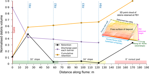
A LiDAR (light detecting and ranging) sensor captured 3D point cloud data of debris retained behind each barrier after the test, including the deformed barrier mesh. Fig. 10 illustrates normalised debris retention and discharge volumes at various flume locations, including barriers, storage container and runout pad. Debris retained in the storage container is plotted at 0 m, that is the gate location. A design debris volume of 180 m³ was prepared, which is used for normalising retention and discharge volumes. In the storage container, 11% of the initial volume is retained, while 89% flows after opening the gate. The first barrier FB1 retains 47% of initial volume, primarily coarse granular material (Fig. 8(e)). Downstream barriers retain less than 5%: FB2 retains 2·9% (Fig. 8(f)), FB3 retains 4·1% (Fig. 8(g)) and FB4 retains 1·4% (Fig. 8(h)) of the initial volume. Sharp reduction in retention after FB1 can be explained using a sieve analogy. FB1, by working as a sieve, filters most of the coarse-grained material and only allows the finer fraction (<25 mm) to pass through. Debris material overflowing FB1 predominantly contained muddy water (Fig. 9(a)) with a limited quantity of coarser debris solids. Subsequent barriers received a large quantity of finer materials that passed through the mesh, leading to 33·4% volume depositing on the runout pad. The initial 180 m³ debris comprised 40% solids and 60% water. Flexible barriers allow water and fines to drain freely. Cumulative retention volume along the flume informs barrier effectiveness in intercepting debris. This study shows underutilisation of downstream barriers when the first barrier has a large retention capacity relative to design volume. While this study using 180 m³ volume is a record-breaking test, as the largest experiment of its kind in a constructed flume, the flume’s 500 m³ capacity allows for even larger experiments. These future tests are essential to rigorously verify the effectiveness of the multiple barrier system.

In this paper, a newly developed 190 m long and 6 m wide flume facility has been introduced, which is the largest of its kind in the world for modelling mountain hazards such as landslides and debris flows. The capability of this new constructed flume is showcased in this study by investigating the impact of a 180 m³ volume of debris flow against multiple flexible barriers in a large-scale experiment with well-controlled initial and boundary conditions. The interactions between debris flow and multiple flexible barriers are elucidated, focusing on the mechanisms of impact, overflow and retention. The key findings from this study are summarised below.

• The newly established 190 m long and 6 m wide flume effectively models debris flow interactions with multiple barriers, capturing the 3D deformation of flexible barriers during impact, overflow and retention. The fluidisation of debris during propagation, as indicated by measured flow height, basal stresses and pore pressures, provides valuable insights into the dynamics of debris flow. This capability is essential for advancing the physical modelling of debris flows and flow–barrier interactions.

• This study validates existing design recommendations for debris flow impact forces on flexible barriers, using modelled flow volumes up to 180 m³. Impact forces on barriers diminish progressively from the first to the fourth barrier, with the first barrier (FB1) cables experiencing peak normalised tension of 0·76, significantly higher than subsequent barriers at 0·085 and below. This trend, which was observed for the specific test set-up using only 180 m³ volume in this study, underscores the effectiveness of multiple barriers in progressively dissipating debris flow energy and reducing forces in downstream barriers.

• The results reveal that the barrier height to flow height ratio (H/h) significantly governs the overflow landing distance, more so than the Froude number. The analytical equation (equation (2)) can conservatively estimate landing distances, accounting for overflow launch angles. This finding is important for determining appropriate barrier spacing, as reducing H/h from 16 to 2 can increase the landing distance ten-fold, with an associated impact on barrier design and placement strategies.

• The findings from this study highlight the importance of the upstream barrier’s retention capacity in the efficiency of a multi-barrier system in intercepting the design volume of debris flow. The first barrier (FB1) plays a pivotal role by retaining approximately 47% of the initial volume. Understanding this role of upstream barriers in progressive retention and discharge is vital for optimising barrier systems and ensuring effective as well as sustainable strategies for debris flow hazards mitigation.

The newly established 190 m long and 6 m wide flume significantly advances our capabilities in physical modelling of debris flows and flow–barrier interactions. The largest flume test of its kind was conducted in this study with a total debris flow volume of 180 m³. This investigation elucidates the mechanisms of debris flow interactions with multiple flexible barriers. Experimental measurements of flow height, basal stresses and pore fluid pressure along the flume uniquely capture how retention, overflow and discharge at these barriers affect the dynamics of debris flows. Basal stresses and pore pressure measurements along the flume reveal variations in the temporal evolution of debris surges and debris fluidisation ratio due to debris interception, overflow and filtering at upstream barriers. Notwithstanding this advancement in physical modelling, it is recognised that the specific test set-up limits generalisation of findings due to experimental constraints and single flow. Analysis of measured results suggest the need for a stress-dependent factor in future multiple barrier designs to consider the effects of flow volume. Further increases in flow volume are difficult but would be worthwhile to explore. Future investigations can ideally design experiments with larger flow volumes, and different debris compositions and barrier set-ups to comprehensively analyse debris flow impact against multiple barriers and support engineering practice with robust design guidelines.