This paper aims to present a novel method and tool for evaluating the motion resolution of industrial robots, defined as the minimum effective motion increment, to enable behavior-informed design and optimization of high-precision industrial robotic systems.
A high-precision laser interferometer is used to measure the joint motion resolution of a KUKA KR210 R2700 Prime robot, following an improved test procedure derived from the ISO 230 standard and an objective error-based identification method. The resulting joint maps are then used to build a prediction tool, implemented in Python and integrated with RoboDK to propagate joint-level resolution to pose- and direction-dependent end-effector Cartesian resolution estimates across the robot workspace.
Results show that ISO 230 tests can mask intrinsic joint resolution in the micro-step range due to backlash-driven response flattening. The proposed test procedure highlights marked joint-dependent performance, with the first three joints generally exhibiting finer micro-step resolution and more stable step responses than the wrist joints. The Cartesian predictor reproduces measured micro-displacement trends with uncertainty envelopes.
The paper provides an objective and repeatable approach that decouples intrinsic resolution from backlash, and introduces an efficient prediction tool for Cartesian resolution estimation, supporting improved system design as well as robot motion planning and compensation for precision manufacturing tasks.
1. Introduction
In modern manufacturing environments, characterized by increasing product customization and demanding efficiency requirements, Industrial Robots (IR) are increasingly adopted to enhance throughput and operational flexibility Oztemel and Gursev (2020). This trend is reflected by the International Federation of Robotics (2025), which reports global annual installations exceeding 500,000 units over the past years (2021–2024). Although IR are, in principle, well suited to meet the required performance targets, this outcome is not immediate and requires careful, application-specific analysis and evaluation. Specifically, from a robotic system design perspective, deploying an IR is not only a matter of nominal reachability, payload and cycle-time feasibility. Early-stage decisions, such as robot and tool selection, cell layout definition, and subsequent motion planning, require digital tools embedding parametric behavioral models that support informed trade-offs among key objectives, including energy consumption and motion accuracy Papakostas et al. (2011); Sharma et al. (2017). To be practically useful, these tools should be integrable into commercial design and simulation platforms, enabling comprehensive evaluation directly in the robot task (or end-effector) space.
Current industrial simulators and virtual commissioning tools offer advanced kinematic analyses for a wide range of IR models, allowing designers to verify path feasibility and to identify critical conditions such as singularities, collisions and joint-limit violations, thereby supporting the generation of viable robot programs Pollák and Goryl (2025); Zheng et al. (2022); Peta et al. (2023). However, they typically do not provide access to key performance indicators, such as the energy demand associated with executing a given path in a specific workspace region, nor the corresponding positioning errors. This limitation is particularly relevant because most IR performance are inherently configuration-dependent Zhang et al. (2025); Wu et al. (2022). Indeed, the same path may be executed in different workspace regions, or even within the same region under alternative joint configurations. In all cases, joint-level behaviors propagate through the kinematic chain in different ways, leading to distinct task-space responses. For this reason, developing reliable behavioral models and ensuring their broad applicability across operating scenarios within the robot workspace requires detailed joint-level understanding Qiu and Xue (2021).
The described problem has motivated substantial research in past decades, with numerous contributions focusing on either robot energy consumption or motion accuracy. On the energy side, detailed mechatronic power-flow models, established combining theoretical and experimental knowledge, enabled the energy-optimal tuning of motion parameters and supported energy-aware layout optimizations Wang et al. (2025); Gadaleta et al. (2017). In terms of motion accuracy, many compensation strategies were proposed at both the joint and system levels, including model-based calibration, error mapping and sensor-based feedback schemes [the results presented in Cao et al. (2022), Slamani et al. (2024), Wang et al. (2020), Ferrarini et al. (2024) and Cheng et al. (2025)]. These approaches have demonstrated that motion errors can be reduced not only for point-to-point positioning but also during the execution of complex paths. Nevertheless, such paths are typically programmed and compensated as dense sequences of targets and micro-corrections, often without explicit knowledge of the IR effective behavior in the fine-motion scale (Kaltsoukalas et al., 2015; Hou et al., 2023; Kang et al., 2025).
In this context, the robotics literature has devoted limited attention to a key metric, motion resolution, defined here as the minimum motion increment that an IR can reliably execute while keeping the associated error within an acceptable threshold. Unlike accuracy and repeatability, which describe the robot’s ability to reach a target position and reproduce it consistently, motion resolution refers to the smallest displacement that the robot can effectively achieve. For instance, a robot may accurately and repeatably perform macro-scale displacements between programmed targets across the workspace, yet fail to produce distinguishable motion when consecutive targets are spaced only by a few tenths of a millimeter, thereby revealing its intrinsic resolution limit. Prior resolution-oriented works focused mainly on parallel positioning systems (Vissiere et al., 2020, Liang et al., 2023), while only a few references addressed serial manipulators Hammond (2011), but without reaching practical readiness or validations on IR operating in real manufacturing environments. Likewise, the reference standard for IR motion performance, ISO 9283 (1998), focuses on pose and path accuracy/repeatability in the task space and related metrics, but does not address resolution. A direct reference to resolution metric can be found in adjacent domains. Specifically, ISO 230 (2014) includes a procedure aimed at evaluating the Least Increment Step (LIS) of machine tools. In simple terms, the LIS represents the smallest commanded step that still produces a clearly distinguishable machine response. Below this threshold, the commanded increment can no longer be reliably separated from the system’s intrinsic motion variability. Recently, ASME B5.64 (2022) introduced a more detailed methodology for linear positioning systems based on a similar metric, namely, the minimum incremental motion. While these standards offer valuable guidance, they do not directly address the jointed, multi-axis nature of IR. In practical terms, motion resolution becomes critical in robotic tasks that require fine path programming and dense target sequences, i.e. where the commanded trajectory is geometrically complex and the robot must follow many closely spaced targets in the 3D workspace Kaltsoukalas et al. (2015). Typical examples include contouring and surface-related tasks such as robotic machining and trimming (Verl et al., 2019), additive manufacturing (Lettori et al., 2022) and laser-based processes (Ma et al., 2023). In these scenarios, the achievable process quality depends not only on motion accuracy over macroscopic motion segments but also on the robot ability to realize small commanded displacements in a predictable and repeatable manner, particularly when the trajectory entails frequent direction changes and local curvature variations.
In line with previous considerations, although motion resolution must ultimately be quantified in task space, its assessment necessarily originates at the joint level. Here, a first practical obstacle is the limited knowledge regarding the servo-actuated systems embedded in IR joints, whose characteristics are typically not disclosed by the manufacturers. In any case, even when feedback resolution and gear ratio could be retrieved, they would yield only a theoretical resolution value, neglecting the entire chain of effects that influence the motion execution from controller command to actual link-side displacement (Bilancia et al., 2025). Among the most influential contributors are transmission errors and, in particular, backlash, whose magnitude depends strongly on the mechanical architecture of each joint (type of reducer, number and type of transmission elements, wear state) (García et al., 2020).
In literature, many works investigated backlash and transmission performance by testing equivalent servo–reducer units on dedicated rigs under controlled conditions [Qiu and Xue (2021)]. This representation is appropriate only for a subset of IR joints, typically the first three axes, where the motor and reducer are often directly coupled. Wrist joints, by contrast, frequently incorporate additional transmission elements (e.g. connecting shafts with universal couplings, intermediate spur/bevel gear stages, and belt–pulley systems) whose contribution may substantially affect the overall transmission error propagated through the serial kinematic chain. A second line of research addressed backlash at the robot level, estimating its influence from end-effector measurements during commanded motions (Zhang et al., 2023); Slamani et al., 2012; Le Reun et al., 2022). Although direct measurements of the cumulative backlash in task space offer clear advantages, this approach becomes impractical for IR with large workspaces as the outcome is strongly pose-dependent, and collecting a statistically meaningful data set would require repeating measurements across many poses and kinematic configurations.
While both perspectives provide useful insights, they leave a critical gap. Specifically, a general, reproducible method to quantify the minimum achievable incremental motion and the backlash of individual robot joints in their fully assembled configuration is still lacking. Joint-level characterization is essential, as it provides a direct and scalable means to isolate transmission-related phenomena and forms the basis for predicting how joint limitations translate into Cartesian motion capability at the end-effector. Achieving this requires metrology tools able to resolve very small displacements with high accuracy. One option is to instrument the robot with secondary high-performance encoders (Weigand et al., 2021), though this solution is expensive for a single IR and entails significant integration and mechanical constraints. Laser interferometric systems, by contrast, are portable and readily reconfigurable, enabling joint-by-joint measurements with limited setup effort while often delivering superior measurement performance, which makes them particularly suitable for systematic joint testing.
To address the identified gaps, the present work proposes a novel method and tool for the evaluation of IR motion resolution to support the development and tuning of high-precision robotic manufacturing systems. Specifically, it introduces a methodology that can be rapidly applied in industrial settings to evaluate joint-level performance and to develop an efficient motion-resolution prediction tool, embedded in a commercial robot simulation environment, to support performance optimization. The main contributions can be summarized as follows:
Engineering method for joint-level motion-resolution assessment using laser interferometry. Building on ISO and ASME standards, the method is formulated to be objective and industrially relevant, and it extends existing procedures with an improved protocol that isolates both the minimum reliably achievable motion increment and the backlash contribution. Detailed guidance is provided on the experimental setup, measurement best practices, test logic and data processing.
Experimental mapping on a KUKA KR 210 R2700 Prime, with the complete dataset and used robot scripts publicly available to support reproducibility and further benchmarking.
Cartesian resolution prediction tool for the robot end-effector at arbitrary workspace poses, derived from the experimentally identified joint data. The tool is implemented as a set of Python scripts integrated into the commercial software RoboDK, where it leverages the built-in robot kinematic models. By updating the joint datasets, the approach can be extended to a broad range of IR supported by the RoboDK library.
The remainder of this paper is organized as follows. Section 2 describes the experimental apparatus and the setup configurations adopted in this study. Section 3 outlines the proposed assessment methodology, including the definition of the performance indexes, the joint test configurations and procedures and the post-processing workflow. Section 4 presents and discusses the experimental results obtained on the KUKA robot. Section 5 introduces the resolution prediction tool and its validation. Finally, Section 6 provides the concluding remarks.
2. Experimental apparatus
This section describes the test equipment used in the experiments, together with the setups developed to address two distinct objectives: mapping the IR joint motion resolution and assessing the end-effector Cartesian motion resolution for final validation. The first setup will be recalled in Section 3 to support the discussion of the adopted testing procedures, whereas the second one will be used in the context of Section 5 for verifying the correctness of the proposed predictor.
2.1 Equipment overview
The used research equipment consists of the following:
A KUKA KR210 R2700 Prime IR, with a rated payload of 210 kg and a reach of 2700 mm. The robot is governed by a KUKA KRC4 controller running KUKA system software version 8.3.25. As for the joint actuation, the motor and transmission characteristics of the six joints are summarized in Table 1. During testing, robot motions were programmed using standard KUKA Robot Language instructions (i.e. PTP for joint motions and LIN for end-effector linear motions). The KUKA Trace function was enabled to record joint positions and motor torques throughout the experiments.
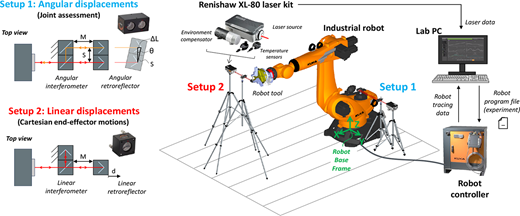
A Renishaw XL-80 laser interferometer system, namely a high-precision metrology instrument capable of measuring linear or angular displacements based on the specific optical kit (interferometer and retroreflector) installed. The XL laser source, typically mounted on a tripod, generates an extremely stable laser beam that passes through the interferometer, and is reflected by the retroreflector. Depending on the available space and operational constraints, either the interferometer or the retroreflector can be fixed to the movable component, while the other must be fixed to a stable rigid reference. The laser parameters are continuously optimized using the XC-80 environmental compensator, which monitors ambient temperature, humidity and atmospheric pressure, thereby ensuring the highest measurement accuracy (0.5 ppm, as specified in the datasheet).
The data was sampled in real time and retrieved at the end of each experiment in the form of arrays. Specifically, the KUKA Trace function samples joint data every 12 ms and stores them into .r64 files, whereas the laser system operates at sampling rates of up to 50 kHz, with data temporarily stored in the internal buffer and then retrieved on the controlling PC via the Renishaw acquisition software, i.e. either Carto Capture or Dynamic Measurement (see Renishaw (2026) for further details). The former supports up to 6,000,000 data points but limits continuous recording to approximately 2 min at the default acquisition rate of 50 kHz. To enable longer acquisitions, Dynamic Measurement allows the sampling rate to be adjusted, though with a reduced storage capacity of 2,047,916 data points. In this work, the experiments required continuous monitoring for 15–30 min; therefore, data was acquired using Dynamic Measurement with the sampling frequency () set to 1 kHz. The recorded data is then saved in .rtx format.
2.2 Setup description
With reference to Figure 1, the following setups were implemented:
Setup 1
For joint assessment and performance mapping, the angular measurement optics were employed to measure the rotation of each individual robot joint. Details regarding the optics installation are provided in Section 3. In all cases, the retroreflector was selected as the moving element, while the interferometer was mounted on a dedicated stage and supported by a second tripod. This configuration helps to prevent measurement errors associated with interferometer tilting, which can reach approximately at rotation angles of . From the initial configuration, where the optics are arranged in parallel, each rotational motion of the retroreflector produces a differential optical path , from which the corresponding rotation angle can be computed as , being S the baseline separation distance, as illustrated in Figure 1. Particular attention must be paid to the Dynamic Measurement software settings, which by default apply a small-angle approximation (). This option was explicitly disabled as it would introduce a non-negligible computation error for larger angles (up to for ). According to Renishaw specifications, the overall angular measurement accuracy, expressed in µrad, can be estimated as , where is the relative angle measured and M is the distance (in m) between the interferometer and the retroreflector.
Setup 2
In this configuration, linear measurement optics were used to measure translational displacements of the end-effector along the X, Y and Z axes of the robot base frame (shown in Figure 1). The system outputs the relative linear distance d traveled by the retroreflector from its starting position, namely where it is located at a distance M from the interferometer. The resulting measurement accuracy, expressed in µm, can be estimated as , where is the relative displacement (in m) measured. According to Renishaw’s technical documentation, linear measurements can be influenced by a so-called dead path error, arising from variations in the unmeasured section of the beam. This effect becomes negligible when mm or when ambient conditions remain stable throughout the entire test. As both conditions were satisfied in this study, the nominal accuracy reported above can be considered valid.
Before each measurement, a meticulous optical alignment procedure was performed in both setups to ensure proper alignment between the interferometer, the retroreflector and the laser beam. The alignment consisted of adjusting the position and orientation of the optical components until an adequate reflected signal intensity was obtained. This procedure ensures that the measured linear or angular displacement accurately represents the actual motion of the target system (either the output link of a joint or the end-effector), thereby minimizing uncertainties due to the setup geometric misalignment.
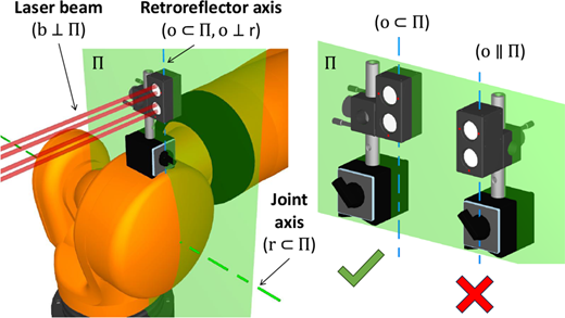
In Setup 1, the retroreflector was mounted on each joint in a configuration designed to minimize beam divergence and prevent signal loss, thereby promoting stable data acquisition over an angular interval of at least . In this regard, the retroreflector should be placed such that its centroid lies on the joint axis of rotation. However, since this condition is not always feasible, as illustrated in Figure 2, in the current setup the retroreflector’s principal centroidal axis o was arranged to lie in a plane passing through the joint axis of rotation r and orthogonal to the laser beam b. It should be noted that if this condition is not satisfied, even small angular movements of about may cause the beam to diverge from the XL detector, resulting in a complete loss of signal.
3. Robot resolution assessment method
This section presents the methodology developed to evaluate the IR joint resolution using interferometric technology. The proposed workflow has been developed considering the setup described in Section 2, though it can be adapted to any articulated robot. The process includes defining performance indexes, configuring the optical setup on the robot, describing the experimental procedures and outlining the post-processing and data analysis approaches.
3.1 Performance indexes
In the field of precision robotics, IR performance assessment is commonly conducted in accordance with ISO 9283 (1998), which primarily focuses on accuracy and repeatability metrics. While the prescribed procedures are suitable for evaluating responses to nominal motion commands (pose reaching and path following) of conventional amplitude, they do not explicitly address motion resolution at the joint () or end-effector (X, Y, Z) level. To overcome this limitation, the present work relies on ISO 230 (2014), originally developed for machine tools, and adopts LIS as the reference performance index for resolution assessment. This index, also referred to as minimum incremental motion [see ASME B5.64 (2022)], represents the smallest displacement that the system can reliably execute within a specified time interval. In the present work, the LIS is identified as the smallest commanded displacement that produces clearly distinguishable motion steps in the measured response. To enable a quantitative characterization of the LIS, the step size error is here introduced, which for joint motions can be defined as follows:
being the commanded joint displacement and the measured one. The angular notation is adopted here because the present study focuses on a serial IR with exclusively rotary joints; however, the same concept directly applies to linear joints (e.g. in Cartesian manipulators). Moreover, equation (1) can be extended to end-effector motions by adopting the corresponding linear displacements and . Expressed as a percentage, can be compared against a predefined acceptability threshold (i.e. a permitted error ), thereby enabling an unambiguous quantification of the LIS.
The LIS of an IR depends on several factors, including the digital resolution of the adopted positioning feedback sensors (encoders or resolvers), the implemented numerical control algorithms and the physical characteristics of the robotic joints, such as transmission type and operating conditions. Among the transmission characteristics, backlash represents a particularly relevant factor in the assessment of motion resolution and must therefore be carefully considered during experimental evaluation. At joint level, backlash at a reference joint position is evaluated by exploring a narrow interval around it through n sequential step motions. Specifically, each position () is reached from opposite approach directions (positive vs negative rotation). According to ISO 230 (2014), the reversal error is then evaluated as follows:
The obtained reversal error can be attributed to backlash only when the two approach motions correspond to opposite load directions in the transmission. In practice, this requires a change in the sign of the motor torque between the forward and reverse motions. Under this condition, the transmission alternately engages opposite flanks of the drivetrain, so the lost motion due to clearances is effectively captured by the reversal measurement.
3.2 Joint test configuration
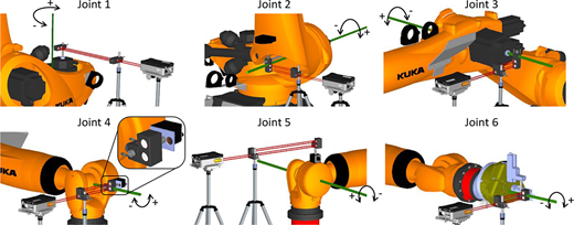
To evaluate the joint resolution and backlash of the considered KUKA robot, Setup 1 described in Section 2.2 and illustrated in Figure 1 for joint 1 was replicated for all robot joints. Particular attention was devoted to the positioning of the angular interferometer and retroreflector, respectively fixed to the ground and to the robot, to maintain stable visibility and prevent signal loss during angular motion. Moreover, to maximize measurement accuracy, their reciprocal distance (M in Figure 1) was kept as short as possible. To meet these requirements, a dedicated arrangement was implemented for each joint. With reference to Figure 3, the adopted solutions are summarized below:
Joint 1: The retroreflector was mounted on the motor housing to place it as close as possible to the joint rotation axis r (green line) and within the reference plane (see Figure 2 for details). A custom adapter was required because the motor housing provides a M32 threaded hole, whereas the Renishaw cylindrical support has an M8 threaded end. The arranged adapter provided an M32–M8 interface and ensured a secure, repeatable mounting. Due to the robot base geometry, the interferometer could not be placed closer than 500 mm.
Joint 2: The M8 threaded hole of the cable holder on the robot link was used as the anchoring point, with no adapter required. Two cylindrical supports of the Renishaw kit were mounted in series to offset the retroreflector from the link and ensure optical visibility throughout the test. A slight centroid misalignment with respect to the reference plane limited the measurable angular range to approximately , without affecting the experiments, since the required range was . The M distance was kept below 200 mm.
Joint 3: The retroreflector was mounted on the motor housing, similarly to joint 1. As in this case, the joint rotation axis coincides with the motor axis, an adapter aligned with this common axis allowed the centroid to lie on the reference plane . Owing to the short lever arm, nearly the full angular range of was achieved. The M distance was below 150 mm.
Joint 4: As joint 5 was set to to vary the load conditions on joint 4 during the experiments, the retroreflector could not be mounted on the end-effector. A magnetic base was therefore attached to the external housing of joint 5 and used to hold a steel plate with an M8 threaded hole, onto which the cylindrical support was screwed. The assembly was aligned perpendicular to joint 4, and the retroreflector position was adjusted along the support until its centroidal axis o lay on the reference plane . The interferometer was placed at approximately 250 mm.
Joint 5: The magnetic base used for joint 4, featuring an M8 threaded hole, was mounted on the joint housing and the cylindrical support was screwed onto it. Although the optics could not be placed close to the joint rotation axis r, the retroreflector was aligned so that its centroidal axis o lay on the reference plane , ensuring stable beam visibility. The maximum M distance was approximately 250 mm.
Joint 6: The retroreflector was mounted on the robot gripper tool, which provides M8 threaded holes for fastening the cylindrical support. The retroreflector was then adjusted along the support to align it with the joint rotation axis r. This configuration enabled the full measurement range of . The interferometer was placed at approximately 200 mm.
These arrangements provided a robust and practical basis for the experimental campaign, allowing measurements to be performed consistently across all joints. It should be noted that, although the specific setup described above was tailored to the KUKA robot considered in this work, the methodology is intended to be broadly portable. When extending this approach to other manipulators, the hardware setup will depend on the robot’s specific mechanical interfaces and materials. However, the geometric alignment criteria detailed in Section 2, together with the experimental procedures described below, remain unchanged, thereby ensuring measurement integrity regardless of the robot model.
The tests were planned to limit experimental effort while still collecting the information needed to characterize the system. The total number of tested configurations is given by , where is the number of joints of the used IR, is the number of discrete angular positions sampled within each joint angular range. Overall, this resulted in 30 configurations for both LIS and backlash evaluations, which are listed in Table 2. During testing, once a given configuration from the table was set, a single joint was moved in a series of small incremental steps via PTP commands, as described in the next section. Notably, LIS was tested for both positive and negative rotations (as shown in Figure 3), yielding two distinct values. To minimize the dynamic effects, the movement speed was set to a low value (0.1% of the maximum).
3.3 ISO test method
According to ISO 230 (2014), the LIS test for each robotic joint consists of performing three consecutive sequences of ten discrete angular position increments. The first and third sequences are executed in the positive joint direction, whereas the second in the negative joint direction, thereby introducing two direction reversals. A stabilization pause of 5 s is applied after each step to allow the system to reach a steady state before the next movement. In this way, a single test typically requires less than 3 min for completion. The step amplitude is kept constant within the test (30 movements) and is then progressively increased from one test to the next until a clear and repeatable displacement is observed in the measured data. The standard does not explicitly prescribe whether the commanded increments should be absolute or relative motions, nor does it specify the angular positions from which the test should start. As a result, additional implementation and programming choices are left to the operator. As specified above, in the present work the experiments were conducted considering the joint configurations listed in Table 2.
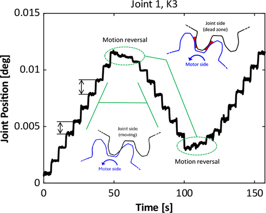
A representative outcome of this test is shown in Figure 4, where the measured signal (Joint 1 positioned at K3 ) exhibits a staircase-like profile. The test is considered acceptable when all the steps appear regular and clearly separated. Nonetheless, the interpretation retains a degree of subjectivity, since the criterion for considering a step “clearly distinguishable” depends on the operator’s judgement. As a result, slightly different resolution limits may be obtained by different analysts, even under identical experimental conditions. Furthermore, from the plot in Figure 4, the following points emerge:
Flattening at motion reversals: this is mainly caused by the reducer backlash and torsional compliance, which absorb part of the actuated displacement before any output motion becomes visible [resulting in the so-called dead zone Ahangarian Abhari et al. (2019)]. Then, once the gear train is fully engaged, the stepped profile exhibits distinct and well-resolved steps.
Irregular step amplitude: although individual steps are clearly defined and distinguishable, their measured amplitude does not always match the nominal commanded value, resulting in a noticeable . The reported staircase profile alternates between larger and smaller steps, which can be attributed to the controller action. This effect is particularly evident when the motion is commanded via absolute position commands, namely, the default option in most IR programming environments.
Overall, the reported ISO approach may not be fully suited to IR, given the mechanical characteristics of the transmission elements typically installed in their joints (see Table 1). Although the procedure can potentially identify the smallest reliably achievable displacement, the resulting LIS also reflects backlash, as its evaluation inevitably includes the steps occurring at direction reversals. Consequently, the intrinsic joint motion resolution may be difficult to isolate, particularly at small amplitudes (Zhang et al., 2023), motivating the adoption of a more robust procedure to decouple the LIS from backlash effects.
3.4 Proposed test method
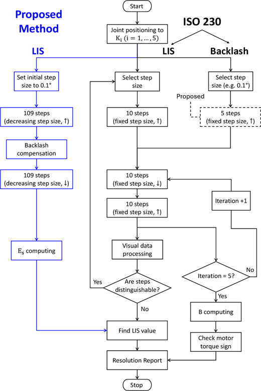
With respect to the ISO procedure described above, the proposed approach addresses the identified limitations through the following main changes:
Evaluation approach: The LIS is determined from data processing rather than visual judgment by considering the step size error . Specifically, the LIS is defined as the smallest commanded step whose measured response satisfies .
Variable step size: During the single test, is decreased exponentially. It spans values from 0.1 down to over 109 steps, with commanded increments defined by , where is the initial step size and i is the iteration index. This profile ensures high data density in the small displacement region, promoting a robust and detailed characterization of the joint response. With a dwell time of 5 s at each step, the full sequence takes under 15 min, whereas the ISO test takes about 3 min for a single step size (so testing all the 109 step sizes would exceed 300 min).
Relative motions: To minimize the controller influence on the executed motion, the increments are set as relative motion commands. Specifically, the i-th increment is added to the measured joint position rather than to the previously commanded position. On the KUKA platform, this corresponds to using the AXIS_ACT_MEAS state variable, which reports the latest drive feedback. This approach prevents deviations from the previous step from propagating to the next one, so each displacement is executed independently and the joint resolution can be characterized more clearly.
Backlash removal: Within each test, all increments are executed in the same direction to avoid joint reversal. The opposite direction is evaluated in a separate test using the same procedure. In addition, a preliminary move in the test direction is performed to remove any mechanical play before the resolution test begins.
To facilitate comparison between the two test procedures and better visualize these aspects, their main characteristics are reported in Table 3, whereas the corresponding flowcharts are shown in Figure 5. In both cases, the experiments start with the initialization of both the robot controller and the laser system. The corresponding robot program is loaded on the controller, and the acquisition parameters (sampling frequency, test configuration and total experiment duration) are defined on the Dynamic Measurement software interface. The laser acquisition time is typically set slightly longer than the expected test duration to ensure that no data is lost during the experiment.
3.5 Backlash assessment
The LIS index does not fully describe the joint motion resolution, as it does not account for the response at direction reversals. To interpret the flattening phenomenon observed in Figure 4 and quantify joint backlash, a dedicated experimental campaign was carried out, similarly to the work presented in Ref. Zhang et al. (2023). In this complementary test, based on ISO 230 (2014), after reaching the target joint position (K1 to K5) and completing the laser alignment, the joint is commanded to execute ten consecutive steps in one direction, followed by ten steps in the opposite direction. To maximize the laser measurement accuracy, which depends on as described in Section 2.2, a preliminary sequence of five steps may be performed to center the subsequent motions around the laser-aligned configuration (, shown in Figure 1). This 20-step cycle is repeated five times consecutively adopting absolute motion commands, as prescribed by the ISO standard. The procedure prescribes a fixed step size but does not indicate a reference value. Therefore, a step size of was selected (one order of magnitude higher than the declared maximum backlash of the commercial reducers installed in robot joints, see Table 1), resulting in a total angular excursion of . To better illustrate these passages, the flowchart of the backlash evaluation test is reported in Figure 5.
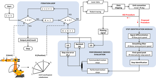
3.6 Data post-processing
The post-processing converts the raw data into the performance indexes introduced in Section 3.1 through a structured, multi-step workflow. The procedure, illustrated in Figure 6, involves importing and organizing the source files (.rtx for laser data, .r64 for robot tracing), filtering and smoothing the signals, detecting the measured motion steps, reconstructing the commanded ones, and finally evaluating the corresponding indexes. The data set is imported into a matrix structure, with each column corresponding to a specific experimental run. In Figure 6, the processing loop iterates every position (K) on each joint (J).
The first processing step (named Data Clipping in the schematic) isolates the time window associated with the current experiment. When the laser acquisition is stopped manually, the saved file contains the full laser buffer, which can include residual samples from previous tests in addition to the current run. This selection is performed based on the duration of the robot trace, which provides the time frame of the test. The corresponding portion of the laser signal is then extracted, and all preceding or trailing sections are discarded. After unit conversion, the workflow splits into two branches: one aimed at estimating the LIS under ISO guidelines (visual approach), and a second dedicated to computing and B as a basis for evaluating the LIS.
The former branch directly produces all the plots of the laser signal, whereas the latter contains further signal processing stages. In particular, the laser signal is first differentiated to obtain joint velocity. Because differentiation amplifies high-frequency noise, a LOWESS (locally weighted scatterplot smoothing) filter is applied using a window corresponding to 500 Hz (), which suppresses oscillations with periods shorter than 2 ms. The result is a smoother velocity signal where each peak corresponds to the transition between two steps. Such peaks are not searched globally, which may identify false positives due to noise or irregular sampling intervals. Instead, the algorithm searches for peaks locally within short time windows. Each window is centered at the expected time of the next movement, located 5000 samples ahead (5 s of dwell time at kHz).
Within each window, the algorithm detects candidate maxima in the velocity signal and selects the most significant one (typically the highest) as the true motion event. After identifying the valid peaks (corresponding to the number of performed steps, see Figure 5), their indices are stored in a vector that defines the start and end of each step. For every detected interval, the algorithm isolates the stationary points corresponding to the stable end of each step. Once all measured displacements () are identified, the step size error is computed as in equation (1), namely by subtracting the commanded values (). The resulting curve is then analyzed to determine where the exceeds a chosen threshold, typically 10% as per ASME B5.64 (2022), providing an objective criterion to evaluate the LIS index. If a different tolerance is required, the threshold value can be adjusted accordingly, yielding a new joint resolution consistent with the selected accuracy level.
Regarding the backlash calculation, except for the two extremal angles of the explored interval around the target position, which are reached only from one direction, the measured forward and backward values, , are averaged across the five repetitions, yielding the two arrays () and (). Using equation (2), is computed at each point and averaged over n points to obtain the reversal error B. To ensure that the reversal corresponded to a real change in gear engagement, therefore including the backlash effect, the motor torque of the investigated joint was recorded via the KUKA tracing function. Only cases associated with a torque sign inversion are considered valid for the backlash evaluation.
This comprehensive post-processing pipeline enables the extraction of consistent and repeatable performance indexes from interferometric data, effectively linking raw experimental signals to the robot’s actual motion resolution.
4. Joint performance mapping
This section presents the experimental results of the resolution assessment performed on the KUKA robot, following the methodology described in Section 3. The evaluation was carried out on the 30 configurations reported in Table 2, and both the LIS and backlash indices were computed for each configuration. Due to space constraints, only a selection of representative plots is included in the manuscript, while the complete data set is provided as supplementary material.
4.1 LIS results
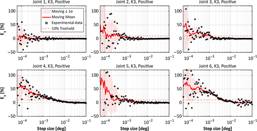
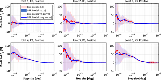
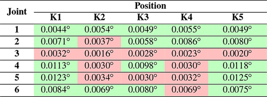
Regarding the LIS, the results were obtained following the test procedures described in Sections 3.3 and 3.4. Under the ISO-based approach, a single LIS value was determined for each configuration by applying the visual criterion defined in the standard. In contrast, the proposed test method provides two LIS estimates per configuration, corresponding to positive and negative motions. As illustrated in Figure 6, the proposed method extracts the step error , which is then plotted as a function of the commanded step amplitude. The results are shown on a logarithmic scale, which linearizes the exponential trend used during the test to execute the 109 steps (see point 2 in Section 3.4) and facilitates comparison across the full range of step sizes. Figure 7 presents the outcome obtained at the median configuration (K3) for each joint. Here, the circle markers denote the discrete values of from the measured data, the solid red line represents the moving mean computed over an 11-point window, and the shaded red band denotes the standard deviation () of with respect to the mean curve. In Figure 7, the selected threshold (10%) is indicated by the horizontal red dashed line. The intersections with the mean curves directly determine the corresponding LIS values. Such values, obtained for all tested configurations (see the supplementary material for data sets related to K1, K2, K3, K4, K5), are reported in Table 4, together with the ISO-based results for comparison. For completeness, the table also includes the ideal LIS values, derived from the characteristics of the actuation modules reported in Table 1. Specifically, these values are computed from the motor feedback resolution and the reduction ratio (e.g. for joint 1), and represent the limiting resolution under purely ideal conditions, i.e. assuming perfect control, motor behavior and reducer transmission. The substantial discrepancy between these idealized values and the measured results further emphasizes the need for rigorous experimental evaluation.
The selection of a 10% threshold for follows the recommendations in ASME B5.64 (2022), although this parameter remains adjustable to suit application-specific requirements. A sensitivity analysis on this parameter indicates that the LIS values are relatively robust to looser tolerances. For instance, increasing the threshold within a reasonable range produces only a marginal reduction in the estimated LIS, due to the steep rise of the error curve, as visible in Figure 7. Nevertheless, if the threshold is set excessively high, for example above 25%, the system’s aleatory uncertainty becomes dominant.
Apart from the final LIS values, further observations can be extracted from the reported plots. In particular, the associated standard deviation complements the stepwise error analysis by characterizing the operating range in which the joint preserves repeatability and positional fidelity. A small standard deviation identifies conditions where the response is consistent across repetitions, whereas increased variability suggests the presence of noise or dynamic effects that degrade the effective resolution. From the reported trends, it can be observed that as the commanded step size decreases, the corresponding error becomes more oscillatory, which is reflected in an increased standard deviation. In addition, a recurring behavior on joints 1, 3, 4, 5 and 6 indicates a tendency to execute steps that are slightly larger than the commanded values. Joint 2 follows the same overall trend, but exhibits a higher standard deviation for small steps, likely due to the counter-balancing system, which introduces a variable and poorly predictable contribution under both static and dynamic conditions, as described in KUKA (2026). Designed to compensate gravitational loads, this device modifies the torque distribution around the joint and introduces nonlinearities in the motion response. As a result, the overall behavior of joint 2 deviates from the trend observed in the other joints, particularly for small commanded steps where the balancing effect can become dominant.
In general, the differences observed across joints can be primarily attributed to the transmission layout and the load conditions of the motor–reducer units installed on each axis (see Table 1). The first three joints feature a compact drivetrain with direct motor–reducer coupling and higher reduction ratios. Consequently, a given commanded motor displacement produces a smaller angular motion at the joint output. Conversely, the wrist joints employ remote actuation through longer transmissions and lower-ratio reducers, so identical motor commands result in larger joint displacements. As a result, achieving a comparable joint-level resolution on the wrist axes would require smaller effective motor-side micro-motions. Regarding the motors, although two different models are adopted for the first three joints and for the wrist joints, they share the same feedback system and drive technology, so their small-scale motion capabilities are expected to be comparable.
Among the tested axes, joint 1 exhibits the lowest LIS and standard deviation. This behavior can be attributed to its higher reduction ratio and to its vertical arrangement, as it rotates about an axis aligned with the gravity direction. Unlike joints 2 and 3, joint 1 does not directly counteract gravitational loads from the robot structure. Consequently, during small and slow step motions the torque demand is largely governed by friction and inertial effects. This reduces the influence of non-linear elastic deflections in the drivetrain, resulting in a more stable and repeatable response. As evident from Table 4, all joints exhibit a similar behavior over their angular range, although their reflected load varies consistently from K1 to K5.
A general remark is that the axis orientation of joints 1–3 is essentially fixed (joint 1 vertical, joints 2–3 horizontal), whereas joints 4–6 can, in principle, assume many spatial orientations within the robot workspace, causing the reflected load to vary substantially with pose. This variation can affect friction conditions and servo behavior, and thus the measured LIS. Consequently, to obtain a design-relevant and accurate assessment, the test on wrist joints should be performed in task-specific configurations representative of the intended process, so that the identified behavior reflects real operating conditions. Further considerations on LIS are provided in the following discussion, in connection with the backlash results.
4.2 Backlash results
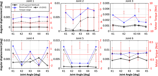
Backlash becomes most evident during motion reversal, when the internal clearances within the reducers (joints 1–3) and, more generally, within the entire transmission (joints 4–6) are engaged. As the mechanical behavior of these transmissions is not consistent across their entire working range as largely discussed in Bilancia et al. (2025); Qiu and Xue (2021), the backlash was also assessed over the full set of 30 configurations, following the procedures reported in Sections 3.5. The obtained results, namely the value of B calculated as explained in Section 3.6, are plotted for all positions (K1 to K5) in Figure 8. To ease interpretation and facilitate comparison, the sample plots report the LIS values discussed above and listed in Table 4. Motor torque from the KUKA tracing is also shown on a secondary axis, with the zero-torque level indicated by the horizontal red line. A change in the torque sign marks the motion reversal and helps identify when the reducer crosses the clearance region and starts to re-engage under load. Therefore, tests in which the torque does not exhibit any sign change (see, e.g. joint 3) are not considered conclusive. A clear indication of whether the executed tests satisfy the torque criterion is provided in Table 5, where the cell color indicates the test validity.
From the observation of the reported results, the following considerations can be drawn:
Joint 1: torque inversion is clearly detectable at all tested angular positions. The corresponding backlash is consistent across configurations, ranging from to , which suggests stable reducer re-engagement.
Joint 2: the experiment was performed with the robot arm in an extended configuration to reduce the influence of the counter-balancing system. A torque inversion appears in four out of the five trials (K1, K3, K4 and K5). However, it is difficult to determine with certainty whether the reducer fully re-engaged in these cases. The estimated backlash ranges from to .
Joint 3: no sign inversion is observed in any configuration, indicating that the measurements are not conclusive for backlash identification.
Joint 4: sign inversion is observed only for K1, K3 and K5, with corresponding backlash values between and .
Joint 5: sign inversion is observed only for K1 and K5. In both cases, the backlash is slightly above .
Joint 6: the torque inversion is clearly visible in four configurations, with the only exception of K4. The backlash ranges from to .
Overall, the presented results reveal a clear joint-dependent trend in backlash. The largest values occur at joints 4 and 5, consistent with the longer transmission chains (with the two motors mounted behind link 3) and the associated accumulation of clearances. By contrast, joints 1 and 2 exhibit lower backlash, plausibly due to the shorter mechanical transmissions, where the motor pinion directly meshes with the reducer input gear. Joint 6 lies in an intermediate range, whereas joint 3 remains inconclusive. The observed behavior is qualitatively consistent with the results in Zhang et al. (2023), which shows similar profiles especially for joints 1, 2, 5 and 6. The slightly lower backlash values in that study are reasonably explained by the smaller robot size (KUKA KR 120 R2500 Prime). Partial agreement is also found with Yao et al. (2025), which investigated a different robot brand but of comparable size (210 kg payload and 2700 mm reach). In that case, although a single backlash value is reported per each joint, the magnitudes are consistent with those listed in Table 5.
As a final remark, when backlash is effectively captured, the two LIS curves are clearly separated in the plots (see, for instance, joints 1 and 6 in Figure 8). In these cases, the ISO-based estimate is influenced by backlash and tends to follow its trend. Nevertheless, the ISO LIS typically remains lower than the backlash magnitude because, even within the dead zone, small but nonzero increments are still distinguishable in the plots due to partial elastic recoveries, and these increments are therefore retained by the ISO visual identification procedure. Conversely, when backlash is not clearly detectable (see joint 3, or more generally the conditions corresponding to the red cells in Table 5), the two LIS curves remain close, indicating that the two methods converge to comparable values. Overall, these outcomes clearly highlight the need to carefully isolate LIS from backlash during joint assessment, otherwise the resulting LIS estimates may incorporate backlash-related effects rather than the joint intrinsic unidirectional motion resolution.
5. Cartesian resolution prediction tool
This section focuses on estimating the smallest achievable Cartesian displacement of the end-effector for a specific robot configuration. In common industrial task-space programming, robot motions are typically planned and specified in Cartesian space, whereas joint-level resolution provides limited insight into the effective positioning capability at the end-effector. As a complete experimental assessment of the robot Cartesian resolution over the entire workspace would be prohibitively time-consuming, requiring multiple physical reconfiguration of the measurement setup for each new robot configuration, the proposed predictor leverages the joint-resolution mapping reported in Section 4 to estimate the Cartesian resolution along the X, Y, and Z axes of the robot base frame (see Figure 1). To bridge joint and Cartesian spaces, a commercially available kinematic solver with an open Python interface (RoboDK) was used.
5.1 Prediction workflow
The prediction tool was implemented as a set of Python modules executed within RoboDK, which provides robust kinematic models for a wide range of commercial IR directly accessible through its official Application Programming Interface (API) RoboDK (2026). Starting from a RoboDK station containing the selected KUKA robot model, the user specifies the robot kinematic configuration directly in the visual interface and then runs the script. The overall framework follows a two-stage pipeline, consisting of joint-level probabilistic modeling based on experimental data and Cartesian prediction through kinematic propagation. The script performs the following passages:
Data import: The experimentally identified joint step size errors are automatically imported and rearranged into a 60 × 109 matrix, where each row represents a single scenario from Table 2 for either positive or negative rotations. In this way, is mapped for every joint, commanded increment magnitude, joint-angle sector and motion direction.
Fitting and modeling (joint space): As the imported exhibits nonlinear trends and sector-dependent variability (K1–K5) within the same joint due to local geometric effects, and becomes increasingly dispersed for smaller commanded steps (see Figure 7), a probabilistic model from the gpytorch library was adopted to represent both the expected and its uncertainty. A Gaussian Process Regression (GPR) was selected for this purpose, as it can capture smooth nonlinear behavior without imposing a predefined functional form. To account for the input-dependent variance observed in the experimental data, a heteroscedastic formulation with a Radial Basis Function kernel was adopted Ozbayram et al. (2024). For each joint and motion direction, the corresponding model takes as inputs the commanded step size and the joint sector (K1–K5), and returns a mean prediction of together with its standard deviation, as shown in Figure 9. Overall, this results in 12 GPR models, which are exported as joint-specific look-up tables. During Cartesian prediction, these are queried via a 2D interpolation routine with conservative boundary handling to avoid extrapolation beyond the experimentally identified domain.
Cartesian predictor (end-effector space): Starting from the specified robot configuration (previously defined by the user in RoboDK and retrieved automatically through the API in Python), the Cartesian predictor simulates the execution of incremental translations along the six directions , and of the robot base frame. For each direction, it evaluates a sequence of commanded step magnitudes, starting from 1 mm and then decreasing exponentially at each iteration. At every iteration a target pose is generated by applying a pure translation to the current pose (orientation unchanged). The RoboDK inverse kinematics solver is recalled to compute the corresponding ideal joint increments. These are then corrected using the joint-level GPR model, yielding realistic joint increments consistent with the measured . The updated joint configuration is finally propagated through forward kinematics to obtain the end-effector displacement.
Monte Carlo aggregation and resolution estimate: To rigorously account for the intrinsic variability of joint behavior (well defined in the established GPR models), the above propagation is repeated over multiple Monte Carlo runs. As the GPR model already provides a Gaussian predictive distribution, repeated sampling enables the corresponding Cartesian output distribution to be reconstructed efficiently. In this context, a sampling size of 50 runs was selected as sufficient to obtain stable estimates and extract statistics. Further increasing the number of runs neither changes the predicted results nor improves accuracy, but only adds redundant samples from the same underlying distribution. For each direction and commanded step size, a summary statistic of the signed Cartesian error (e.g. mean, standard deviation and min/max envelope) is produced. A Cartesian LIS value is then derived by identifying the smallest step sizes for which the predicted execution error remains within a prescribed tolerance band (), expressed in relative terms with respect to the commanded displacement.
Results export and visualization: results are automatically exported as text files for post-processing and can be visualized directly within the Python environment. An example of the resulting output is a set of direction-dependent resolution curves, which relate the commanded Cartesian step size to the expected relative execution error (with associated uncertainty bounds) for a given robot configuration.
This procedure ensures that the probabilistic characteristics of the joint behavior are preserved and propagated into the Cartesian prediction stage. To support reproducibility, the complete RoboDK station is provided as supplementary material, with all scripts encapsulated in the project and the corresponding look-up tables included.
5.2 Validation and discussion
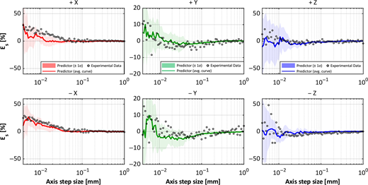
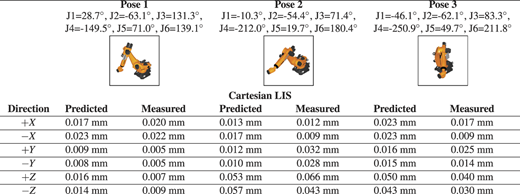
To validate the proposed predictor, three robot poses were randomly selected within the workspace. For each pose, six independent tests were performed using the Setup 2 in Figure 1 (linear retroreflector mounted on the end-effector). In each test, the robot was commanded in Cartesian space through a series of linear displacements (LIN commands) along a single base-frame direction (, , , , or ). The commanded displacement magnitude was initialized to 1 mm and then exponentially reduced at each iteration, while the end-effector orientation was kept constant. All the performed motions were recorded, and the resulting Cartesian error profiles were subsequently compared with the predicted ones. This comparison evaluates both the predicted mean trend and the associated uncertainty, verifying whether the model reproduces the measured drift and dispersion of the executed motion. Figure 10 reports the results obtained at pose 1, while those related to the remaining ones are provided in the supplementary material. Figure 11 summarizes the Cartesian LIS values obtained for all poses. From the reported plots, a key qualitative consistency with the joint-space mapping results of Section 4 is evident. In particular, for sufficiently large commanded steps the error evolution is locally repeatable, whereas for smaller steps the dispersion increases considerably, indicating a transition to a more variable behavior. This same pattern emerging in Cartesian space supports the central assumption of the framework, namely that joint-level stochastic behavior, identified experimentally and modeled via the GPR, can be propagated through the robot kinematics to predict the Cartesian resolution of the end-effector.
Across the three poses, the predictor generally provides a good match to the measured Cartesian behavior. Specifically, the model slightly underestimates the drift for steps between mm and mm along , while most measurements remain within the predicted standard-deviation bounds, confirming the usefulness of the Monte Carlo uncertainty estimate. Along and , the agreement is excellent, with all points contained within the envelope and aligned with the predicted mean. For , the model tends to overestimate the dispersion at small steps, whereas for it correctly captures the rapid increase in variability for commanded displacements below mm. At pose 2, corresponding to a more extended robot kinematic configuration (see Table 6), the measured dispersion increases, especially along the Z direction, where reduced stiffness is more pronounced Wu et al. (2022). Finally, for pose 3, agreement remains strong overall, with isolated deviations for very small commanded steps along the X direction. Overall, these experiments indicate that the proposed tool can estimate the Cartesian LIS with consistent accuracy across different robot poses. Importantly, the predictor captures both the execution error trend and the configuration-dependent variability that dominates at small commanded steps, which is essential when using the tool to quantify task-space resolution.
The potential of this information for achieving superior performance in precision tasks (primarily through path planning and compensation) is evident from a direct comparison with position-accuracy results previously observed for the same robot model on larger-scale movements during simulated machining trajectories. Taking pose 1 as reference, the measured Cartesian LIS ranges from 0.005 to 0.022 mm across the tested directions (see Table 6), with the maximum occurring along . In Ref. Ferrarini et al. (2024), for a 1 m straight line along the direction at 50 mm/s, the maximum oscillation amplitude was 0.139 mm and, together with trajectory drift, yielded a total orthogonal position deviation of 0.442 mm at the end point. Although these macroscopic deviations are much larger than the LIS, they should be interpreted with respect to the loop cycle time of the implemented compensation module, which in that case applied corrections every 4 ms. In the referenced work, the corrective actions ranged between 0.002 and 0.006 mm in the orthogonal direction (namely, the Y and Z axes). Relative to pose 1, these values are comparable to, or even lower than, the measured LIS along those directions, indicating that the robot cannot reliably execute all the compensations. This is also reflected by the final residual deviation of 0.073 mm, which remains larger than the corresponding LIS value. These practical examples highlight the advantage of modeling the robot behavior in advance, thereby enabling enhanced control performance through predictive path generation and compensation.
Finally, the current implementation of the Cartesian predictor does not explicitly account for backlash, since it operates under the assumption of small unidirectional Cartesian motions, which consistently correspond to small unidirectional joint motions. Within these narrow intervals, the commanded linear movements do not cause joint-level reversals. From a mechanical standpoint, as long as the reducer remains engaged on a single flank, the transmission dead zone does not affect the output motion, ensuring numerical consistency between the model and the experimental evidence. Including backlash into the predictor would certainly improve the representation of joint-level behavior. However, this would also raise important practical issues. First, a complete experimental assessment over the six joints and multiple operational zones may not always yield conclusive results, as observed in this work for Joint 3 (see Table 5). This condition may also vary across robot types and models. More importantly, to fully exploit the experimental backlash data within the predictor, a reliable dynamic model is required to estimate joint torques accurately and identify sign inversions. While such capabilities may be available in brand-specific simulators (e.g. ABB RobotStudio), they are generally unavailable in third-party software environments such as RoboDK.
6. Conclusions
This paper reports on advances in the assessment and prediction of IR motion resolution, which is a key parameter for the design and performance optimization of high-precision robotic systems, as it directly determines the achievable path fidelity and process quality. Adopting ISO/ASME standard approaches as a reference, the study showed that their direct application to articulated robots can be problematic in the micro-step range, mainly because backlash effects at direction reversals that can mask the intrinsic joint resolution. To overcome this, a rigorous, joint-level methodology that defines resolution as the smallest increment that can be effectively actuated according to an objective step-error criterion is proposed. Using a laser interferometer and an improved test sequence with high granularity in the small-step region, the method isolates intrinsic resolution by avoiding reversals during the resolution test, while backlash is quantified separately through a dedicated procedure supported by torque-sign monitoring. In addition to improving robustness and repeatability, the protocol proved operationally efficient, reducing the experimental effort by about 20 × compared to the referenced standards while providing finer insight where resolution transitions occur. The experimental mapping on a KUKA KR210 R2700 Prime highlighted strong joint-dependent behaviors consistent with drivetrain architecture: the main axes generally exhibited finer intrinsic resolution than the wrist axes (i.e. Vs. ), while backlash was larger on joints with more complex transmission chains (up to for joint 5).
Beyond joint assessment, the paper introduced a model-based resolution prediction tool that extends joint results to Cartesian space. Joint-level step-error data was modeled probabilistically and propagated through robot kinematics using RoboDK and Monte Carlo sampling, enabling pose- and direction-dependent estimates of end-effector resolution together with uncertainty envelopes. Validation against measurements at three randomly selected robot poses confirmed that the predictor reproduces both the mean trends and the increase in dispersion at very small commanded steps. As the tool is embedded in a robotic simulation environment, it supports informed choices at early design stages regarding workstation layout and further improves robot motion planning and compensation for high-precision robotic systems before deployment. Despite the promising results, the current tool remains limited to translational Cartesian predictions along the X, Y and Z directions, while orientation-related resolution is not evaluated. Moreover, its validation has so far been restricted to a single robot model. Future work will therefore address rotational motions and extend the validation to robots with different kinematic architectures, including tests under dynamic payloads and other application-specific operating conditions.
The joint data set, robot test scripts and Python prediction tool related to this work are made available to support reproducible evaluations and promote further developments.
Supplementary material
The research dataset related to this work is freely accessible at the following Mendeley Data repository available at: Link to the cited article