Bunker price forecasting is an important task in the shipping industry. Many researchers have contributed to bunker price forecasting using deep learning (DL) models, but have not applied dimensionality reduction techniques (DRTs) to enhance the model accuracy and efficiency. This study proposes a novel hybrid model for forecasting Rotterdam HSFO 380cst prices by combining two DRTs with a deep neural network (DNN).
This study combines a mean squared error (MSE) filter and principal component analysis with DL models to produce a six-month-ahead forecast (April–September 2025). Moreover, to assess and compare the quality and accuracy of the models' forecasts, this study uses mean absolute error, MSE, root mean squared error and mean absolute percentage error (MAPE). In addition, this study uses the Diebold-Mariano and the Harvey, Leybourne and Newbold tests to test the hypothesis that there is a significant difference between the proposed DL model's forecasts and other DL models.
The experimental results confirm that the proposed method enhances the model's efficiency and accuracy. For example, MAPE for the test data decreases significantly from 8.83% (DL model without DRTs) to 5.17% (DL model with DRTs).
This study combines DRTs with DNNs to build an efficient and robust forecasting model to predict Rotterdam HSFO 380cst prices. The outcomes of this research can be generalised to other complex maritime time series data, such as crude oil and alternative green fuel prices.
1. Introduction
Maritime transport plays a vital role in international trade and the global supply chain. International seaborne trade has been increasing over the past few years. The reasons for this trend are not only the growing population and existing global market needs, but also the constant decrease in maritime transport costs driven by technological advancements.
Bunker cost is one of the main components of maritime transport costs. Besides the large investment in bunker infrastructure, it accounts for 30–70% of operating costs, depending on bunker prices (Notteboom and Vernimmen, 2009; Ronen, 2011; Tran et al., 2025). Bunker prices are of utmost importance to operators, as they heavily affect economic planning and the financial viability of ventures and determine decisions related to compliance with regulations (Stefanakos and Schians, 2014).
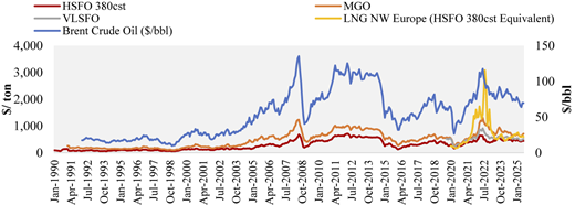
Bunker is the heavy residual product left after refining crude oil into gasoline, kerosene, and diesel. Along with many other factors, the interaction between crude oil supply and demand directly affects the bunker fuel prices. As a result, its price is closely linked to the crude oil price, as shown in Figure 1. However, recent successive IMO sulphur regulations and decarbonisation policies introduced a structural break in bunker fuel pricing by shifting cost formation away from crude oil toward refinery complexity, compliance costs, and region-specific supply conditions. As a result, crude oil prices became an incomplete proxy for bunker fuel costs. In addition, it is affected by the relationship between supply and demand, exhibiting volatility that is related to but inconsistent with crude oil prices (Chen et al., 2022). Ships can use many types of bunker fuels in their voyage from the origin port to the destination port. The heavy sulphur fuel oil (HSFO) 380cst is the most common bunker type used in the shipping industry, with a 3.5% sulphur content. Among many other types, very low sulphur fuel oil (VLSFO) and ultra-low sulphur fuel oil (ULSFO) with a sulphur content not exceeding 0.5 and 0.1%, respectively, meet the recent regulations issued by the International Maritime Organisation (IMO) in January 2020 (IMO, 2022).
As the importance of bunker prices increases, effective forecasting could further benefit shipping operators and other stakeholders in the shipping industry by enabling them to determine sailing speeds, navigational routes, and market-related decisions with compliance issues and financial planning, as well as regulators to estimate the timing and cost of regulation more accurately. However, forecasting bunker prices is not an easy task, even in the short term, which is more appropriate than long-term forecasting, because many factors affect bunker prices, with the rapid changes in shipping cost dynamics, such as crude oil supply and demand, shipping market conditions, pandemics, geopolitical conflicts, and operational factors.
Therefore, this study focuses on providing both business-oriented and academically grounded forecasts that key stakeholders, such as the Suez Canal Authority (SCA), can rely on by constructing a mid-term forecasting model for bunker prices by deep learning (DL), with the following contributions to the literature:
Proving the effectiveness of applying the dimensionality reduction techniques (DRTs) to improve the accuracy and efficiency of the DL models' forecasts;
Showing the superiority of the proposed DL model with DRTs over both the DL-based models without DRTs and statistical-based autoregressive integrated moving-average with exogenous variables (ARIMAX) models.
Evaluating the effectiveness of the proposed model using four accuracy evaluation measures; and
Comparing the predictive accuracy of four pairs of ARIMAX and DL models' forecasts using Diebold-Mariano (DM) and Harvey, Leybourne, and Newbold (HLN) tests.
In summary, this study addresses two unresolved gaps in bunker price forecasting. First, although DL models have been increasingly applied to forecast bunker and crude oil prices, limited attention has been paid to systematically integrating DRTs with DL frameworks to enhance both forecasting accuracy and computational efficiency, particularly in a mid-term forecasting context of the Rotterdam HSFO 380cst price. Second, beyond conventional accuracy metrics, this study formally evaluates forecast superiority using DM and HLN tests, thereby providing statistically grounded evidence of performance differences between DL-based and econometric models. To address these gaps, this study proposes a hybrid DL model combining DRTs (both for feature selection and extraction) and evaluates its performance against ARIMAX and standalone DL models using multiple accuracy measures and formal forecast comparison tests.
The remainder of this paper is organised as follows: Section 2 reviews the relevant literature. The research methodology is described in Section 3. Section 4 presents the empirical results of the modelling construction for six-month-ahead forecasts of Rotterdam HSFO 380cst prices. Finally, Section 5 presents the conclusion and future research.
2. Literature review
This section provides a detailed literature review to gain broad insights into DL-based and statistical forecasting methods of bunker prices, as well as the practical usefulness of DL across various research domains.
2.1 DL applications in various fields
DL has established itself as a transformative technology across a wide range of fields because of its ability to automatically extract complex patterns from large datasets. It is widely applied in various fields, including data science, engineering, robotics, healthcare, medical sciences, computer science, finance, transport, manufacturing, and industrial automation. DL serves as a highly effective, robust, and versatile approach across numerous practical applications, such as image, speech, text, and face recognition, as well as outlier detection.
Abbas et al. (2023) developed a convolutional mixer algorithm to address face occlusion in face recognition. Sakas et al. (2023) proposed a hybrid agent-based and system dynamics model with a feedforward neural network to simulate key performance indicators in transportation within supply chain firms. Biliškov and Papić (2024) designed a non-invasive method using image pre-processing and deep learning to detect marine litter from unmanned aerial vehicles, promoting healthier marine ecosystems. Chang et al. (2024) developed advanced DL and ML algorithms to predict financial trends, assess risk, and forecast stock prices, focussing on the technology sector to identify the most accurate and efficient predictive models under varying conditions. Natarajan et al. (2025) tackled challenges in automatic speech recognition, aiming to preserve speech quality and enhance intelligibility. Villa et al. (2025) trained a custom DNN on a synthetic dataset of diverse local fringe structures and noise profiles. Zhu and Xie (2025) proposed a distributed control strategy using an adaptive sliding-mode controller for a 13-degree-of-freedom cooperative robotic system in automated fibre placement.
While our study focuses on deploying a hybrid DNN mechanism to forecast bunker prices, DNN enables researchers in the maritime sector to enhance the route choice modelling. For example, Zhuang and Chen (2022) developed a multi-task long short-term memory (LSTM) model based on automatic identification system (AIS) ship-trajectory big data to propose an autonomous generation for ship route selection. Meanwhile, Nakashima and Shibasaki (2023) developed ML models for short-term forecasting of weekly dry bulk cargo throughputs using the AIS data. In addition, Chen et al. (2025) employed DNN models to propose a novel ship route choice method that considers factors such as weather conditions and carbon emissions. They initially developed a convolutional neural network (CNN) model to simulate the navigation environment and capture the maritime conditions. Moreover, Latinopoulos et al. (2025) explored two model-free deep reinforcement learning algorithms: (1) a double deep Q network and (2) a deep deterministic policy gradient to determine and optimise the ship route choice regarding the weather, which includes future expected conditions and unexpected shocks of supply chain disruptions.
DL models, including DNNs, CNNs, and LSTMs, consistently capture complex, nonlinear patterns across finance, healthcare, and maritime operations. In the maritime sector, they have been effective for ship route optimisation, cargo forecasting, and environmental monitoring. However, DL models can be data- and computation-intensive, and few studies have explored their integration with DRTs for improved efficiency and accuracy. This study addresses this gap by proposing a hybrid DNN model for bunker price forecasting, extending DL's practical benefits to maritime economic and operational planning.
2.2 DL-based forecasting of bunker price
Many forecasting methods can be applied to predict bunker and crude oil prices, given the strong linear correlation between the two (Abdullah and Zeng, 2010). In this subsection, we summarise classical statistical and econometric techniques, as well as artificial intelligence (AI)-driven techniques used to forecast bunker prices.
First, regarding classical statistical forecasting, Alizadeh et al. (2004) proposed appropriate futures contracts for hedging bunker price fluctuations. They investigated the hedging effectiveness of these contracts using both constant and dynamic (time-varying) hedge ratios and compared their effectiveness. Stefanakos and Schinas (2014) suggested a methodological approach for forecasting marine fuel prices. They applied a vector autoregressive moving-average process and forecasted a tetra-variate and an octa-variate time series of bunker prices, resulting in good agreement with the actual values. Moreover, Stefanakos and Schinas (2015) examined the applicability of well-known fuzzy time-series forecasting techniques to predict weekly bunker price time series for four major world ports (Rotterdam, Houston, Singapore, and Fujairah). Choi (2017) used system dynamics to carry out a medium- and long-term forecasting analysis of bunker prices. He established a quantitative analysis based on a causal loop diagram of the variables that affect bunker prices. Chen et al. (2022) examined how future crude oil prices imply bunker prices by co-integration analysis with constructing vector error correction, autoregressive moving-average (ARMA), ARMA with exogenous variables, and vector autoregressive models to determine which model best predicts the long-run equilibrium between bunker and crude oil futures prices. Zulu et al. (2022) deployed an ARIMA model to predict bunker fuel prices from 2022 to 2032, and the results showed that ARIMA (1,1,2) provides the best fit, with smaller errors than simple, double, and triple exponential smoothing. Heen (2023) used ARIMAX models to forecast crude oil prices, showing that including exogenous variables improves accuracy. Mati (2023) highlighted that incorporating geopolitical events, such as the Russian-Ukrainian war, into ARIMAX enhances forecasting accuracy by accounting for external shocks.
In particular, several studies have used monthly datasets to construct mid-term forecasts of crude oil prices. Baruník and Malinská (2016) modelled the monthly term structure of crude oil futures via a dynamic Nelson–Siegel framework combined with a time-delay neural network, generating 1-, 3-, 6-, and 12-month-ahead forecasts. Al-Gounmeein and Ismail (2021) analysed monthly Brent prices using long-memory and volatility models, showing that hybrid autoregressive fractionally integrated MA-generalised autoregressive conditional heteroskedasticity (GARCH) models outperform conventional approaches. Anastasiadis and Siskos (2023) employed monthly WTI data to evaluate ARMA-GARCH, ARMA-exponential GARCH, and ARMA-fractionally integrated GARCH models, finding that the ARMA-exponential GARCH (1,20) specification provides the most accurate forecasts.
In addition, many research efforts in forecasting bunker prices use AI-driven techniques, such as ML and DL, because of the complexity and nonlinearity of bunker price data. Given the evolution in computational capabilities, Kanamoto et al. (2019) proposed a new method to predict freight indices using DL and AIS data. The simulation results showed that the Baltic Capesize index can be predicted with high accuracy, and that introducing AIS data in the prediction is effective. Kim (2021) conducted a short-term predictive analysis of Singapore HSFO 380cst using three DNN models: a recurrent neural network (RNN), an LSTM, and a gated recurrent unit (GRU). Yan et al. (2021) employed principal component analysis (PCA), multidimensional scaling, and locally linear embedding (LLE) methods to reduce data dimensionality and built eight models to forecast crude oil spot prices using the RNN and LSTM models. Açık and Doymuş (2022) studied volatility spillovers among the prices of major fuel centres worldwide. They used an integrated causal structure in variance and interpretive structural modelling, including a marine gas oil (MGO) price dataset for eight fuel centres used worldwide: Fujairah, Hong Kong, Houston, Istanbul, New York, Piraeus, Rotterdam, and Singapore. Kim et al. (2022) built short-term models for forecasting liquefied natural gas (LNG) bunker prices using RNNs and performed predictive analysis with simple RNNs, LSTMs, and GRUs. Wang et al. (2023) proposed a hybrid forecast model, an ensemble empirical mode decomposition-CNN-improved LSTM, to forecast daily crude oil futures prices on the Shanghai Energy Exchange in China. Arola Rusman et al. (2023) compared ARIMAX with GRU and LSTM models, finding that while LSTM captures complex patterns better, ARIMAX remains competitive due to simplicity and interpretability. Lu and Huang (2024) proposed a novel hybrid model within the decomposition–integration paradigm to forecast crude oil prices, combining mixed-frequency CNN, bidirectional LSTM, and generalised autoregressive conditional heteroskedasticity models. The empirical findings for West Texas Intermediate (WTI) and Brent crude oil indicate that the proposed approach outperforms other models across evaluation indicators and statistical tests and demonstrates good robustness. Tan et al. (2024) applied a multiscale time-series decomposition learning framework on monthly oil prices, successfully modelling both short- and long- term fluctuations.
Statistical models (e.g. ARIMA, ARIMAX, and GARCH) consistently capture linear trends and provide interpretability, while AI-driven models (DNN, RNN, LSTM, GRU, and hybrids) excel at modelling nonlinear patterns and complex dependencies. Limitations include statistical models' inability to handle nonlinearity and AI models' high data and computational demands. For example, Kim (2021) concentrated on short-term forecasting of Singapore HSFO 380cst prices using recurrent DL architectures but did not address feature redundancy or model efficiency. Chen et al. (2022) examined the long-run equilibrium relationship between bunker and crude oil futures prices using cointegration-based econometric models but evaluated forecasting performance mainly within a traditional statistical framework, without assessing the potential gains from nonlinear DL models, advanced feature engineering, or out-of-sample predictive accuracy tests. Arola Rusman et al. (2023) compared ARIMAX with GRU and LSTM models but did not incorporate dimensionality reduction or conduct formal hypothesis testing of forecast differences. Therefore, a clear gap remains in combining DRTs with DL for more efficient and accurate bunker price forecasting, which this study addresses by proposing a hybrid DNN model benchmarked against ARIMAX and standard DNN approaches.
In summary, DL models, including DNN, RNN, CNN, and LSTM, have been widely used in recent years, and their effectiveness has also been confirmed in the maritime industry. However, research on the efficiency of applying DRTs and their combination with DL models was insufficient. Therefore, this study proposes a new method that combines a DL model with DRTs, leveraging both feature selection and extraction techniques to forecast Rotterdam HSFO 380cst prices. Moreover, to confirm the validity of the proposed method, we use the ARIMAX model as a benchmark and the DL model without DRTs. In addition, this paper uses two hypothesis tests to confirm the significant difference between the forecasts generated by the proposed model and other statistical and DL models.
3. Research methodology
3.1 Basic concept
The philosophical idea of AI, dating back to McCarthy et al. (1955), is becoming a reality today. The growth of AI is attributed to the emergence of ML systems that learn from data, particularly DL, a family of ML algorithms that uses DNN as a form of brain-inspired computing (Shlezinger and Elder, 2023). In ML, a computer program is given a set of tasks to complete, and the machine learns from its experience if its measured performance on these tasks improves over time, as it obtains more practice completing them; thus, the machine makes judgements and forecasts based on historical data (Taye, 2023). The DL model is a network of neurons with multiple parameters and layers between the input and output. DL uses neural network topologies as its basis. Consequently, they are known as deep neural networks (Schmidhuber, 2014).
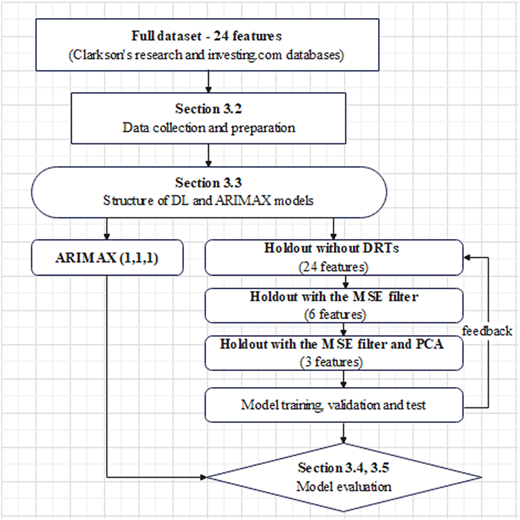
The model development flowchart used in this study is shown in Figure 2. The model in this study targets a six-month-ahead forecasting (April–September 2025) for Rotterdam HSFO 380cst prices, considering the decision-making process of key stakeholders: for example, the SCA periodically reviews and adjusts its pricing and marketing policies every six months, including (1) canal tolls, (2) canal surcharges applied to certain ship types, and (3) rebate navigational circulars issued to specific vessel types. This semi-annual cycle allows the SCA to incorporate recent developments in global trade, bunker fuel prices, freight markets, and competitive routes, while avoiding excessive volatility or uncertainty for shipping lines. This frequency also aligns with shipping companies' medium-term planning horizons and contract cycles, enabling informed adjustments to canal tolls, surcharges, and rebate schemes without disrupting traffic predictability. Since all these pricing schemes are often assessed on a semi-annual basis using monthly-collected indicators, this study uses monthly data, considering the core business needs and decision-making context of the respective stakeholders. Daily or weekly data tend to be excessively noisy for strategic planning, while monthly forecasts provide the clarity required for budgeting and tariff decisions, although we consider our method applicable to shorter-term forecasts with daily or weekly data for other stakeholders, such as ship operators engaged in bunker procurement.
The initial steps in model development are to collect the dataset and prepare the data for analysis by imputing missing values and standardising the data. Then, DL models are constructed with the full dataset of 24 features as the input layer and a mean square error (MSE) filter, followed by principal component analysis (PCA) to reduce data dimensionality and improve DL model efficiency, producing more efficient outputs and better forecasts.
In addition to DL models, this study examines the ARIMAX model as a representative statistical benchmark that can incorporate exogenous variables, unlike ARIMA. Including ARIMAX with the same explanatory factors as in our proposed method provides a conventional point of comparison, enabling a systematic evaluation of model performance. Notably, we use a single representative ARIMAX model (i.e. ARIMAX (1,1,1)) rather than testing a large number of alternatives based on Akaike information criteria and Bayesian information criteria, and forecasting accuracy measures, while still effectively capturing the key dynamics of Rotterdam HSFO 380cst prices.
The following subsections address: data collection from reliable maritime and business-oriented portals and the subsequent data preparation process in Section 3.2, the design structures of the ARIMAX model and the three DNN models with carefully selected hyperparameters suited to the relatively small sample size in Section 3.3, and the implementation of two evaluation schemes, one based on forecast accuracy measures and another on hypothesis testing to assess predictive performance in Sections 3.4 and 3.5. These comprehensive methodologies and outputs provide decision-makers with more reliable and interpretable forecasts to support strategic pricing and policy planning in maritime operations.
3.2 Data collection and preparation
Data preparation is a fundamental stage of data analysis. Various techniques must be applied to make the data suitable for forecasting, depending on the nature of the data (Zhang et al., 2003). This study relies on Clarkson's research intelligence portal and the investing.com database to extract time-series records. The dataset consists of 213 monthly time series records (from January 2008 to September 2025) and includes 25 variables (one target variable and 24 features).
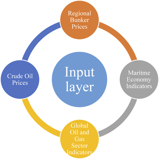
Table 1 shows the 24 features initially included in the analysis. Clarkson's research intelligence portal and Investing.com were used to extract monthly time series of the features selected in the analysis. To enhance model transparency and reproducibility, the 24 explanatory variables are selected through a structured, domain-driven feature identification process grounded in established fuel-price dynamics and maritime economy indicators. As shown in Figure 3, input features are grouped into four thematic categories reflecting the main drivers of marine fuel markets: (1) regional bunker price indicators, capturing spatial price differentials across major bunkering hubs, such as Rotterdam, Singapore, Fujairah, and Houston; (2) maritime economy indicators, represented by Baltic exchange indices that proxy global shipping demand across dry bulk, clean tanker, and dirty tanker segments; (3) global oil and gas sector indicators, represented by energy-related equity indices, such as S&P Oil & Gas Exploration & Production and Dow Jones Oil & Gas Producers, which reflect broader market expectations and sector-level price shocks; and (4) crude oil benchmarks, including WTI and Brent, given their strong upstream influence on refined marine fuels. This set was chosen to ensure (1) comprehensive coverage of supply-chain price drivers, (2) avoidance of redundant variables, and (3) availability of consistent monthly data over the study period. This systematic categorisation supports interpretability and ensures that the model captures both upstream oil-market fundamentals and downstream maritime-sector dynamics.
We use average imputation to handle missing values by averaging the entire dataset. The other problem is the existence of high variation in the dataset; thus, we apply standardisation by transforming the original data into the z-score with zero mean and unit-variance distribution, as shown in Equation (1):
where z: standardised value of the data, x: original value of the data, : mean, and : standard deviation.
3.3 Structure of DL and ARIMAX models
This study employs 24 explanatory features, including bunker prices, stock market indices, crude oil benchmarks, and Baltic indices, whose interactions are highly nonlinear and difficult to capture with traditional linear models. DL are well-suited for such tasks as they can automatically learn complex, nonlinear relationships from high-dimensional data and have been shown to outperform linear models in energy and financial forecasting (Yu et al., 2019; Fan et al., 2021; Zhang et al., 2018). Therefore, the choice of DL is driven by both the complexity of the multi-source feature space and the nonlinear dynamics of energy and financial markets.
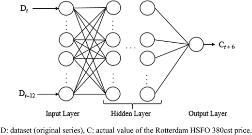
As shown in Figure 4, this study inputs the past six months from the current value and outputs Rotterdam HSFO 380cst prices six months ahead. A linear function is applied to the input and output layers, and a rectified linear unit (ReLU) function is applied to the intermediate layers as an activation function. Table 2 presents the DNN architecture, consisting of three fully connected hidden layers with ReLU activation functions. Input features are standardised using z-score normalisation, and the model minimises MSE as the loss function. Training is conducted with the Adam optimiser; a small batch size of 4 is chosen to improve model generalisation, as it allows more frequent weight updates, which is beneficial for the relatively limited dataset. The model is trained for 100 epochs, based on monitoring training and validation loss curves that indicate convergence around this point; early stopping is also applied to prevent overfitting. Dropout (0.2) and batch normalisation are applied across all layers to reduce overfitting and stabilise convergence. The input layer includes 24 features, and the output layer uses a linear activation function to forecast the continuous Rotterdam HSFO 380cst price. This design balances model complexity and dataset size, ensuring robust training dynamics, generalisation, and high forecast accuracy.
Moreover, as shown in Figure 4, we use the past 12 months to forecast 6 months ahead, as hits period captures important information, including potential cycles, medium-to long-term trends, and seasonality in the time series (Hu et al., 2015).
This study adopts the Holdout method, an approach to out-of-sample evaluation in which the available data are partitioned into three segments: training, validation, and test sets, as shown in Figure 5 (Sammut and Web, 2017). Training and validation data are used to develop the forecasting model, and then the model accuracy is confirmed using test data. Table 3 shows the data partitioning using the Holdout method. Similarly, the ARIMAX (1,1,1) model is partitioned into training (70%), validation (10%), and test (20%) sets, with the training set used to estimate model parameters and the validation and test sets reserved for out-of-sample evaluation.
3.4 Evaluation criteria and DRTs
To evaluate the accuracy of the DL models, we use MSE, mean absolute error (MAE), root mean squared error (RMSE), and mean absolute percentage error (MAPE), as expressed in the following equations (2) to (5), respectively (Garg et al., 2022).
where i: iteration; n: sample size; ei= (): error term; : observed series; and : estimated series.
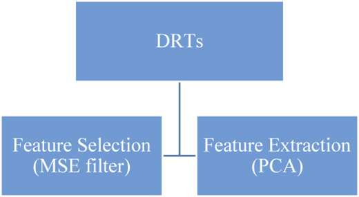
To address the problem of high dimensionality of the dataset (24 dimensions) and to enhance modelling accuracy and efficiency, this study applies the MSE filter and PCA as distinct DRTs, as shown in Figure 6.
Using the MSE filter, we evaluate the importance of input variables with DL. This study represents the value “0” as a forcibility input for each variable and runs the simulation using a validation dataset. The importance of a feature is estimated by calculating the impact of the model's prediction error after the feature is reordered. If the model error increases when the feature values are replaced, the feature is important because the model relies on the feature to make predictions. If feature values do not change the model error, the feature is unimportant.
PCA is a statistical method used mainly to reduce a cases-by-variables data table to its essential features, called principal components (PCs). PCs are linear combinations of the original variables that maximise the variance explained by all variables (Greenacre et al., 2022). Information is measured by the total variance of the original variables, and the PCs optimally account for most of that variance (Pearson, 2010). The PCs have geometric properties that allow for an intuitive and structured interpretation of the main features of a complex multivariate dataset (Hotelling, 1933). PCA aims to explain the variables' variances; thus, certain variables should not contribute excessively to that variance for extraneous reasons unrelated to the research core (Becker, 2020).
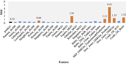
Figure 7 shows the MSE filter results using 24 variables. Six variables are essential in this case because MSE became significantly larger than “predict1” (the base case using all features). Therefore, we decided to use six features (Korea_ifo380, Fujaira_MGO, S&P_Oil&Gas_Exploration&Production, Dow_Jones_Oil&Gas_Producers, Dow_Jones_Oil&Gas, and Crude_Oil_Brent) as an input layer in DL models.
In addition, after experimental analysis, we applied PCA as a feature extraction technique to reduce dimensionality and achieve a good fit for the target variable. Korea_ifo380, Fujaira_MGO, S&P_Oil&Gas_Exploration&Production, Dow_Jones_Oil&Gas_Producers, and Dow_Jones_Oil&Gas have been combined into two PCs, while keeping Crude_Oil_Brent out of the PCA because of its strong direct relationship with all bunker prices, including our target. Then, we can evaluate the robustness of the extracted two PCs regardless of the crude oil price effect. The two PCs reflect 92% of the variation in the original data. Therefore, we reduce the dataset from six to three dimensions.
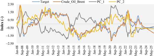
Tables 4 and 5 and Figure 8 show the results of PCA executed to enhance the DL models' forecasts. Figure 8 shows that oil-driven dynamics strongly explained the target series before 2014, but structural breaks and post-2020 market disruptions led to a persistent decoupling, suggesting that linear and oil-based models lose explanatory power in the later period. PC_1 represents the dominant long-run energy and market cycle, showing strong and stable co-movement with both Brent crude oil and the target series during the pre-2020 period. This indicates that PC_1 captures the main systematic variation driving the market and provides substantial explanatory power under relatively stable conditions. In contrast, PC_2 reflects secondary or short-term dynamics. Its behaviour becomes increasingly volatile after 2020, with weaker and less consistent alignment with the target variable, suggesting a diminished and time-varying explanatory role in the post-2020 regime.
In this way, the experimental analysis shows better results by applying both the MSE filter and PCA combined with DL models, as discussed in more detail in the next section.
3.5 DM and HLN tests for comparing the predictive accuracy
This paper uses DM (Diebold and Mariano, 1995) and HLN (Harvey et al., 1997) tests to investigate the robustness of the results and forecasting quality of the proposed model compared with its counterparts. Although the DM test provides good practice, it could be seriously over-sized in the case of two-step ahead prediction (i.e. h = 2), making the problem more acute as the forecast horizon (h) increases; therefore, Harvey et al. (1997) suggested modifying the DM test by adding a bias correction factor besides depending on a student-t distribution instead of a normal distribution.
Although the two tests share the assumption that they are appropriate for any loss function, they differ in other respects. The DM test uses a standard normal distribution table and is better for large sample sizes, while the HLN test uses a Student's t-distribution and is better for small sample sizes.
Diebold and Mariano (1995) suggested a test statistic based on the following formula:
where : the sample mean of a loss-differential series (); : the empirical autocovariance; n: sample size; and h: step ahead forecast. The loss-differential series is defined as follows:
where : observed series; and : estimated series. The empirical autocovariance is defined as:
Then, Harvey et al. (1997) suggested a modification of the DM test statistic to be as follows:
4. Empirical results and evaluation
This section evaluates the effectiveness of the method proposed in Section 3 against selected DL-based and ARIMAX benchmark models.
4.1 Estimation results
Based on the method described in the previous section, we develop an ARIMAX and three DL models as follows:
ARIMAX (1,1,1)
Holdout without DRTs (24 features),
Holdout with the MSE filter (6 features), and
Holdout with the MSE filter and PCA (3 features) – the proposed model.
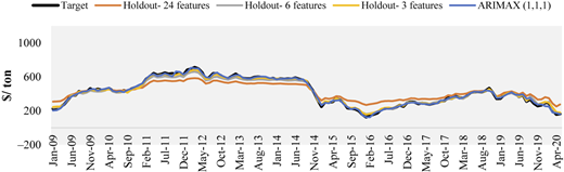
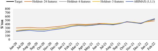
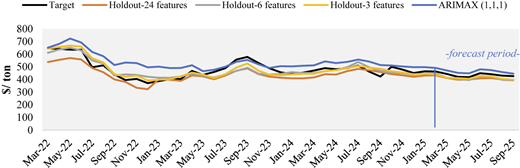
Figures 9 and 10 show the training and validation results of the ARIMAX (1,1,1) and Holdout models. The training and validation results for the model using 24 variables (full dataset) are the least accurate at following the target, while the proposed model with DRTs (3 features) is the closest to the target. Figure 11 summarises the model test results for the forecast outputs of the ARIMAX (1,1,1), DL models, and the observed dataset. Among the four constructed models, the ARIMAX (1,1,1) provides the least accurate fit to the actual time series, while the proposed Holdout-DRT (3 features) model provides the best fit, demonstrating the effectiveness of combining DRTs with the DL for predicting six months ahead for Rotterdam HSFO 380cst prices.
The results of the four accuracy measures (MAE, MSE, RMSE, and MAPE) are summarised in Table 6. Regarding the Holdout models, they give better results if applying the MSE filter than using the 24 features, while they give the best results if adding PCA; for example, MAPE (test data) decreases from 11.44% for ARIMAX (1,1,1) to 5.17% for the proposed Holdout model with DRTs (3 features). This demonstrates that integrating both feature selection and extraction within DL frameworks enhances generalisation ability and yields superior predictive accuracy compared to traditional statistical models.
4.2 Comparing the predictive accuracy of two forecasts
In this subsection, we investigate the robustness of the results and forecasting quality of the proposed DL model compared with its counterparts using DM and HLN tests from the following viewpoints: the proposed Holdout model with DRTs (3 features) versus the other constructed models. Both tests investigate whether there is a significant difference between the forecasts generated from the two predictive models.
First, the DM test is applied to compare the three forecasts for the aforementioned pairs of models using the standard normal distribution table. Moreover, due to the small sample size (n = 43) and the forecast horizon (h = 4), we applied the HLN test using the student's t-distribution table at the 1 and 10% levels of significance, with 42 degrees of freedom. Table 7 shows the output for both tests, confirming the same conclusion.
According to both DM and HLN tests, we conclude that, at the 99% confidence level, significant differences are observed between the forecasts generated from the proposed Holdout with DRTs (3 features) and those generated by both the ARIMAX (1,1,1) and Holdout without DRTs models. In addition, at the 90% confidence level, a significant difference is observed between the two forecasts generated by the proposed Holdout model with DRTs (3 features) and that with the MSE filter (6 features).
4.3 Discussion
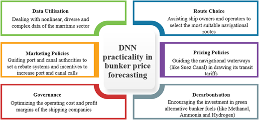
DNN offers a powerful tool for forecasting bunker prices in a volatile maritime fuel market. It is vital in learning complex patterns from large-scale data and adapting to changing market dynamics. Using DNN in bunker price forecasting is crucial for shipping companies, traders, and policymakers who make decisions on fuel procurement or decarbonisation. Figure 12 summarises the practicality of DNN in predicting bunker prices.
In shipping companies, fuel cost is a critical factor. According to Stopford (2009), the share of fuel cost can reach approximately 42% in tramp shipping. Given such a high-cost structure, shipping companies are susceptible to fluctuations in fuel prices. The dynamics of fuel prices significantly impact operational strategies and decision-making processes. When fuel prices rise sharply, companies tend to adopt slow steaming as a cost-saving measure, thereby reducing fuel consumption and overall operational expenditures. Additionally, in fleet deployment planning, greater emphasis is placed on optimising routes and selecting ports of call with improved efficiency. In the longer term, fuel price trends influence capital investment decisions, including the procurement of fuel-efficient new ships and the retrofitting of existing vessels with energy-saving technologies. Thus, bunker prices should not be regarded merely as an item in the cost structure; instead, they constitute a critical external economic factor affecting the broader management of shipping companies. Their fluctuations are strategically significant, directly shaping operational optimisation and ultimately the competitive advantage of shipping companies.
Among various applications of DNN in the maritime sector, route choice modelling stands out as a crucial area. Shibasaki et al. (2017) investigated the share of the Suez Canal route in the global dry bulk shipping market by comparing it with alternative routes, using a comprehensive database of vessel movements. In this study, fuel cost was incorporated as a key input parameter into the route choice model. Since bunker prices are essential for accurately estimating fuel costs, their integration into such models is expected to enable real-time route optimisation and dynamic navigational decision-making. Furthermore, in the context of the Suez Canal, various pricing and marketing policy initiatives have been introduced, such as the design of canal tariffs and rebate schemes for canal transit on specific navigational routes to optimise the canal's market share compared to alternative routes (Suez Canal Authority, 2025). In these initiatives, predictive modelling of bunker prices using DNN techniques may serve as an effective analytical tool, particularly for forecasting future price trends and formulating pricing strategies or transit incentives accordingly.
Another practicality of DNN in bunker price forecasting is to adapt irregularities and nonlinearities in real-world data (e.g. time series, financial data, climate patterns, or maritime operations) that traditional linear models struggle to capture (Fischer and Krauss, 2018; Fan et al., 2022; Jiang et al., 2021; Morales-Ramírez et al., 2025). In addition, there is growing research interest in using DNNs for bunker price forecasting to support decarbonisation, particularly in sectors such as energy, transport, maritime logistics, and industrial systems, by helping in forecasting, optimisation, system control, and decision-making (Samanta et al., 2023; Mahmoud and Ben Slama, 2025; Sun et al., 2025). In this light, bunker price is not merely a cost determinant but a pivotal driver that influences multi-layered decision-making processes, including route selection, policy formulation, and strategic planning. The use of DNN-based forecasting methods is expected to play a central role in advancing smart shipping and realising data-driven maritime operations.
Despite their analytical power, DNNs remain difficult to interpret because of their complex nonlinear architectures (Lipton, 2018). Their performance is also highly sensitive to data quality, variable completeness, and the stability of historical relationships (Zhang et al., 2017). Market disruptions, regulatory shifts, or geopolitical shocks can further limit their ability to generalise in real-world forecasting contexts (Makridakis et al., 2018; Lim and Zohren, 2021). Therefore, DNN outputs should be interpreted with caution, acknowledging these inherent limitations in transparency and data dependence.
While DNNs provide a powerful framework for capturing complex nonlinear patterns in bunker price data, their performance can be challenged by high-dimensional, noisy market data. Integrating DNN with DRTs, a statistical approach for extracting the most informative components from large datasets, enhances forecasting power by reducing noise, mitigating overfitting, and improving model stability. This combination enables practitioners to generate more reliable and actionable fuel price predictions, which are crucial for shipping companies to optimise routes, plan fleet deployment, and manage operational costs. Traders and market analysts benefit from a clearer identification of key price drivers, which support better hedging and strategic decision-making, while policymakers and authorities can leverage accurate forecasts for tariff design, transit incentives, and decarbonisation planning. By focussing the DNN on the most relevant information, DRTs effectively transform bunker price forecasting into a robust decision-support tool, directly linking predictive accuracy with practical operational and strategic benefits in volatile maritime fuel markets.
Our proposed method, DNN-DRTs, enhances bunker price forecasting by extracting the most informative signals from high-dimensional market data, improving accuracy and stability. Accurate and robust forecasting from the proposed method enables SCA to anticipate fuel price trends and proactively adjust transit tariffs or rebate schemes, maintaining competitiveness and optimising revenue. Shipping companies can integrate these forecasts into voyage planning to optimise routes, speeds, and port calls, minimising fuel expenses while maintaining schedules. Similarly, traders and operators benefit from fuel hedging by using these reliable predictions to reduce financial risk, improve cost control, and make data-driven procurement decisions.
5. Concluding remarks
Commercial shipping is the most crucial part of the international trade system. Given the significant contribution of the shipping sector to greenhouse gas emissions, many concerns have been raised about clean bunker fuels as an alternative to conventional fuels. IMO has announced successive regulations since January 2020 on climate change and environmental issues. Due to increasing regulatory restrictions on particle emissions, vessel operators also need access to accurate price information for the different types of bunker fuel.
Bunker price forecasting is an important task in the shipping industry. Efficient forecasting of bunker prices enables stakeholders in the shipping sector to develop and set operational plans, as bunker costs can account for 50% of a ship's operating costs for certain types of ships. Therefore, many studies presented time-series analyses for bunker prices, and both classical statistical-based and DL-based methods were proposed. However, none of these studies adopted any form of DRT in combination with DL models.
This study has successfully achieved its initial objective of constructing a six-month-ahead forecast of Rotterdam HSFO 380cst bunker prices by combining DL models with DRTs. The empirical results showed that the proposed DL models with DRTs outperform other DL models without DRTs and ARIMAX (1,1,1), demonstrating the effectiveness of DRTs in improving forecasting performance. More specifically, this study processed the input data, including missing-value imputation and standardisation, and applied DNN, a simple multi-layered neural network, with an appropriate DL architecture to handle the input dataset. PCA produced two PCs that were orthogonal to the target variable, accounting for 92% of the variation in the five features generated by the MSE filter.
The empirical analysis for the model training, validation, and test showed the benefit of combining DRTs with DL models. All accuracy measures (MAE, MSE, RMSE, and MAPE) achieved better results with the MSE filter than the 24-feature model, and the best results were achieved by adding PCA. According to both the DM and HLN tests, deploying DRTs significantly improved the efficiency and accuracy of model forecasts. Both tests rejected the hypothesis of no significant difference between the forecasts generated by the proposed DL model and other competing DL and ARIMAX (1,1,1) models.
The proposed DNN-DRT model provides actionable insights by explicitly linking model components to business decisions. DRT identifies the key drivers of bunker price fluctuations, guiding strategic planning and risk management. The DNN generates accurate forecasts of future fuel prices, supporting voyage optimisation, route planning, and fuel procurement decisions. Scenario-based outputs inform Suez Canal tariff adjustments and long-term investment decisions, while evaluating using DM and HLN tests ensure the forecasts are statistically robust and reliable for practical use. By mapping each model element to specific operational and strategic decisions, the approach transforms complex predictive analytics into a concrete decision-support tool for maritime stakeholders.
Although the present study offers important insights and provides a useful enhancement to forecasting bunker prices, we have some future work that may further improve our modelling. Plenty of feature selection and extraction techniques for DRTs could be tested and included, such as independent component analysis, linear discriminant analysis, LLE, uniform manifold approximation and projection, low-variance filter, high-correlation filter, and missing-value ratio. Another enhancement could be achieved by changing the DL model structure, such as the number of intermediate layers, the type of loss function, the batch size, the number of epochs, and the input activation function. We may also extend the proposed models presented in this study to directly forecast the prices of other bunker fuels, such as VLSFO, MGO, and LNG. Due to the high correlation between crude oil and bunker prices, we may also extend this work to forecast crude oil prices.