Open-source one-dimensional modelling of piston-effect pressure waves in high-speed railway tunnels: verification, benchmarking against 3D CFD and single-train design-load screening

Symbol

Definition

A, A₀

free/undisturbed tunnel cross-sectional area (m²)

A_tr

train cross-sectional area (m²)

c₀

ambient speed of sound (m/s)

GCI

grid-convergence index (%)

L, L_tr

tunnel/train length (m)

p, p₀

pressure/ambient pressure (Pa)

P_f

initial compression-wave amplitude (Pa)

pobs

observed order of grid convergence (−)

u, V

air/train velocity (m/s)

β = A_tr/A₀

blockage ratio

λ_t, λ_tr

Darcy friction factors (tunnel/train)

Δp_pp

exterior peak-to-peak pressure change (kPa)

E

specific total energy (J/kg)

k₂, k₄

Jameson artificial-dissipation coefficients (−)

γ

ratio of specific heats (−)

Δx

grid spacing (m)

τ

dynamic sealing time constant of the rolling stock (s)

When a train enters a tunnel at high speed, the displaced air generates a compression wave that propagates at the speed of sound; the tail generates an expansion wave, and both reflect at the open portals with a change of sign. The superposition of these waves and of the quasi-steady pressure field around the train produces the unsteady pressure environment known as the piston effect. Its consequences are well documented: alternating loads relevant to the fatigue design of car bodies and tunnel equipment; aural discomfort and, in the limit, medical risk; the micro-pressure wave emitted at the exit portal; and a dominant influence on the required free cross-sectional area of the tunnel, one of the most expensive geometric parameters of a high-speed line (Baron, Mossi, & Sibilla, 2001; Gawthorpe, 2000; Hara, 1961; Howe, 1998; Niu, Sui, Yu, Cao, & Yuan, 2020; Vardy, n.d.; William-Louis & Tournier, 2005; Woods & Pope, 1981).

Train–tunnel aerodynamics has been dominated in the last two decades by three-dimensional CFD with moving-mesh techniques, used to study surface pressures for different tunnel lengths (Luo, Zhang, Zhang, & Zhang, 2017), unsteady subway flows (Xue, You, Chao, & Ye, 2014), car-body fatigue loading during crossings (Lu et al., 2019), slipstreams in double-track tunnels (Fu, Li, & Liang, 2017; Meng, Meng, Wu, Li, & Zhou, 2021) and aerodynamic comfort during passings (Yan, Yang, & Zhang, 2011). The Chinese high-speed programme has driven much of this activity, reviewed by Ma, Zhang, and Liu (2012), and the fluctuating pressure loading of trains in tunnels had been characterised experimentally and numerically before it (Seo, Park, & Min, 2006). These studies resolve the flow in detail but require meshes of tens of millions of cells and days of computing time per configuration, which makes them poorly suited to the repeated multi-case scans – over tunnel length, cross-section, blockage ratio and speed – needed early in the design of a new line.

One-dimensional unsteady compressible models occupy the opposite end of the cost–fidelity spectrum. Since early analytical and flow-prediction methods (Hara, 1961; Woods & Pope, 1981), 1D methods have been refined continuously (Baron et al., 2001; Howe, 1998; William-Louis & Tournier, 2005) and remain the workhorse of practical tunnel aerodynamics, as implemented in software such as ThermoTun (Vardy, n.d.); network models of the same family reproduce measured air-exchange rates in extra-long tunnels within about 7% (Krasyuk, Lugin, Irgibayev, & Alferova, 2023), and 1D formulations remain an active research topic (López González, Galdo Vega, Fernández Oro, & Blanco Marigorta, 2014; Vorobyev & Bogdanov, 2025). Openly available 1D tools do exist, but not for this physics. The Subway Environment Simulation program (SES) (U.S. Department of Transportation, 2002), whose version 4.1 was released from distribution restriction in 2021 and forked as the open-source OpenSES (OpenSES Project, 2022), has been used for decades and is arguably the reference open tool for underground aerodynamics. It is, however, an incompressible, quasi-steady network model developed for subway ventilation, thermal and fire analysis, and it therefore does not represent the sonic-speed propagation, portal reflection and superposition of compression waves that govern loads at 350 km/h. The compressible 1D codes that do represent them – ThermoTun (Vardy, n.d.), and the TETUN and TRUNS codes developed for European certification work and validated against full-scale campaigns (Somaschini, Rocchi, Tomasini, & Schito, 2020) – are proprietary or otherwise not openly distributed. Academic method-of-characteristics implementations are widespread but are generally described rather than released.

The scope of this paper is deliberately restricted to a single train. Both the exterior wave-system loads and, through a first-order cabin-sealing model, the interior pressure relevant to passenger comfort are treated. Two-train crossings in double-track tunnels, which govern the comfort-based sizing of such lines, are the subject of a companion study and are not claimed here. A central methodological point, established by the grid-convergence study of Section 3, is that the area-averaged 1D formulation resolves the localised suction peak beneath the train nose as well as the wave-system quantities, but only on grids an order of magnitude finer in cell size, and some two orders of magnitude more expensive, than wave-system work requires. The parametric study of Section 4 is therefore run at wave-system resolution, and its quantitative claims are confined to the quantities convergent there – the exterior peak-to-peak load and the sealing-filtered interior comfort metrics.

The contributions are: (1) an open-source quasi-1D solver, with derivation and released V&V suite (Section 2, Appendix A); (2) verification against analytical references over a range of blockage ratios, validation of the piston-wind field against a published full-scale measurement, and an independent benchmark of the compression-wave amplitude against published 3D CFD at 250–400 km/h, together with a grid-convergence analysis delimiting the model's valid output (Section 3); and (3) application to the planned 350 km/h North–South railway in Vietnam, reporting grid-convergent single-train exterior loads and, via a cabin-sealing model, interior comfort metrics (Section 4). Section 5 discusses limitations and Section 6 concludes.

Because the physical and numerical formulation used here follows established one-dimensional practice, it is worth stating precisely what this paper claims. The governing equations, the moving-blockage representation of the train and the MacCormack discretisation are not new: they follow (William-Louis & Tournier, 2005; Woods & Pope, 1981) and the wider 1D literature, and no new closure, boundary treatment or numerical method is introduced. Nor is a capability claimed that the proprietary compressible codes lack. What is offered is, firstly, an implementation gap: an openly licensed, documented and extensible compressible solver for high-speed tunnel transients, released with a verification-and-validation suite that reproduces every figure and table of this paper from the published scripts. The open tools in this field are incompressible network models that cannot address this physics, and the tools that can are closed, so a practitioner or researcher wishing to test a new friction law, portal treatment or sealing model against a documented compressible baseline currently has nowhere to start. Secondly, and independently of the software, the paper contributes a methodological result: the grid study of Section 3.4 shows that the localised suction peak beneath the train nose, commonly assumed to lie beyond the reach of area-averaged 1D models, is in fact grid-convergent and quantifies the resolution at which it becomes so. That result corrects a limitation commonly attributed to this class of model – one the present author had also assumed before carrying out the refinement study reported here.

The flow is one-dimensional, compressible and unsteady, with the train represented as a prescribed reduction of the free area A(x,t). With ρ, u, p and E the density, velocity, pressure and specific total energy, conservation of mass, momentum and energy over the free area reads

closed by p = (γ−1)ρ(E − u²/2), γ = 1.4. The geometric term p ∂A/∂x is the axial projection of the pressure force exerted by the train nose and tail on the air; −p ∂A/∂t is the moving-surface work, with ∂A/∂t = −V ∂A/∂x for a rigid train. Wall and train-skin friction use Darcy closures, f_t = −(λ_t/8)ρ|u|u P_t and f_tr = −(λ_tr/8)ρ|u−V|(u−V)P_tr, with λ_t = 0.02 and λ_tr = 0.012 (William-Louis & Tournier, 2005; Woods & Pope, 1981). A formal derivation of (1)–(3), the treatment of the moving blockage and its equivalence to the formulation of Woods and Pope (Woods & Pope, 1981), together with a global energy-balance check, are given in Appendix A. The model contains no local (form) loss coefficients at the nose, tail or portals; the consequences of this choice are quantified in Section 3.4 and discussed in Section 5.

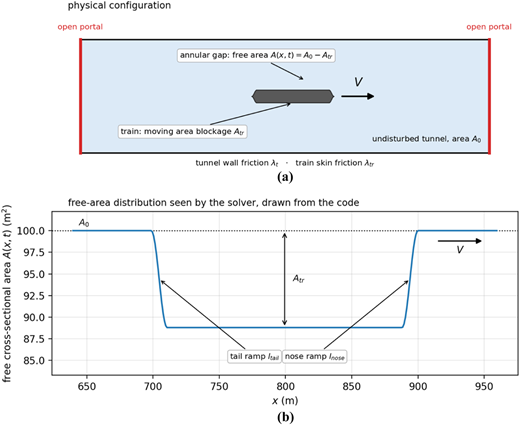
The blockage b(x,t) rises from zero to A_tr over the streamlined nose length and falls symmetrically at the tail using cosine ramps; A(x,t) = A₀ − b(x,t) (Figure 1). The train position is prescribed kinematically, so portal entry and exit are handled by clipping the blockage to the domain.

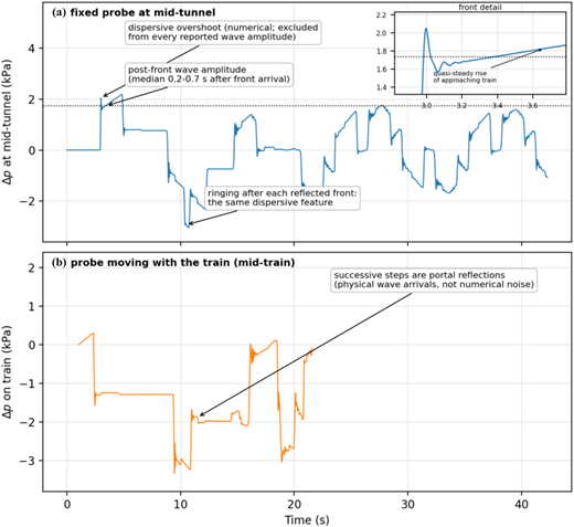
Equations (1)–(3) are integrated with the explicit predictor–corrector MacCormack scheme (MacCormack, 1969), formally second-order in space and time. Because the waves are weak (Δp/p₀ of order 10^–2), shock-capturing is unnecessary; grid-scale oscillations near the area ramps are damped by Jameson-type artificial dissipation with a pressure-based sensor scaling the second-difference term (k₂ = 0.8) and a background fourth-difference term (k₄ = 0.008) (Jameson, Schmidt, & Turkel, 1981); these coefficients are held fixed for every result in this paper, and their influence is quantified in the sensitivity study of Section 3.4. The time step is not fixed: it is recomputed at every step from a Courant condition on the local wave speeds, with a Courant number of 0.60 for the application cases and 0.85 for the benchmark case of Section 3.4, both well inside the explicit stability limit. The formulation carries a general area field A(x, t), so a tunnel of varying cross-section – enlargements, transition zones or shafts represented as area changes – is admissible without modification, although every case presented here uses a prismatic tunnel. At the portals, characteristic-type open-boundary conditions are imposed on two ghost cells at each end: the incoming characteristic is prescribed from the ambient state (ambient stagnation conditions for inflow, ambient static pressure for outflow) while the outgoing characteristics are extrapolated from the interior, which reproduces the sign-inverting reflection at open ends. As is typical of dissipative schemes on a near-discontinuous front, the leading edge of the compression wave carries a small dispersive overshoot; the physically meaningful quantity is the post-front plateau amplitude, which is the value used throughout (the overshoot is examined in Section 3.4). Wherever a wave amplitude is reported, it is extracted as the median pressure in a fixed window from 0.2 to 0.7 s after the front arrival at the probe, which excludes the overshoot by construction; peak-to-peak values, by contrast, are formed from the raw recorded pressure history at a probe moving with the train at mid-train length, as the difference between its maximum and minimum over the transit, without this front treatment; the definition and its consequences are discussed in Section 5. A global energy-budget check on a closed test duct shows the total energy drift to remain within the artificial-dissipation truncation over a full transit time (the quantitative result is reported in Appendix A).

The interior (cabin) pressure p_c is obtained from the computed exterior signature p_e by the standard first-order pressure-sealing relation dp_c/dt = (p_e − p_c)/τ, integrated exactly over each time step, where τ is the dynamic sealing time constant of the rolling stock (τ = 0 for an unsealed vehicle; τ of order 6–18 s for modern sealed high-speed stock). Passenger comfort is assessed from the largest interior pressure change within moving 1 s, 3 s and 10 s windows, compared with the UIC comfort limits of 0.5, 0.8 and 1.0 kPa respectively (CEN, 2021).

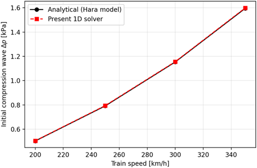
Terminology follows ASME practice: comparison against the analytical entry-wave solution is verification, since it tests the discretisation against an exact solution of the same model, whereas comparison against published 3D CFD is benchmarking rather than validation, because the reference is itself a computation and not a measurement; the comparison against full-scale measurement in Section 3.2 is validation in the strict sense. Table 1 and Figure 2 compares the computed plateau amplitude of the initial compression wave with the analytical entry-wave solution (Hara, 1961), with friction removed to match the analytical assumptions, for two blockage ratios spanning the practical range: β = 0.112 (A₀ = 100 m²) across 200–350 km/h, and β = 0.160 (A₀ = 70 m²) at 350 km/h. Agreement is within 1% throughout, and the amplitude is grid-insensitive (below 0.5% for Δx ≤ 2.5 m); the computed front-arrival time at mid-tunnel matches the acoustic time x/c₀ within 0.3%. The verification therefore holds over the whole blockage range used in the application, not at a single β.

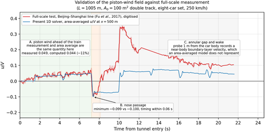
The one quantity for which an independent full-scale measurement could be obtained with all of its parameters documented is the piston-wind field. Fu, Li, and Liang (2017) report a full-scale test on the Beijing–Shanghai high-speed line in which an ultrasonic anemometer recorded the longitudinal air velocity 500 m from the entrance of a 1,005 m tunnel of 100 m² free cross-section carrying two tracks, as an eight-coach trainset passed at 250 km/h, the probe being 1 m from the car body and 1.5 m above rail level. The configuration matches the baseline of Section 4 in free cross-section, track arrangement and trainset and differs in speed. Running the present solver at that configuration and sampling the area-averaged velocity at the same station gives Figure 3.

What is being compared needs care, because the measured and computed quantities coincide over part of the record and not over the rest. Ahead of the train nose, the air column in the tunnel is driven forward essentially as a plug, so a point measurement and the area average are the same quantity; over that interval the computed piston wind is 0.044 V against a measured 0.049 V, low by 11%, and the two traces follow the same rise. The nose-passage transient is reproduced closely: the computed minimum is −0.100 V against a measured −0.099 V, and it occurs within 0.06 s of the measured one; the arrival times of nose and tail follow from the tunnel kinematics. Once the nose has passed, the probe lies inside the annular gap 1 m from the car body and records a near-body boundary-layer velocity, which reaches 0.36 V at tail passage; an area-averaged formulation does not represent that quantity and returns 0.03 V, so the two curves separate by construction rather than by error. The comparison therefore validates the piston-wind field and the wave kinematics against measurement and illustrates directly where area averaging ceases to apply, but it establishes nothing about the interior structure of the annular flow. It is grid-independent: the computed piston wind changes by 0.3% across Δx = 2, 1 and 0.5 m.

As an internal consistency check on the same quantity, the quasi-steady piston wind was also compared with a momentum balance written with exactly the same closures as the solver, which isolates numerical error: for a 1 km train (Atr = 10 m², A₀ = 60 m²) in a 12 km tunnel at 120 km/h the mid-tunnel velocity approaches 5.695 m/s against 5.533 m/s from the balance, a 2.9% difference attributable to finite development time. Because both sides share the friction closure that makes the test sensitive to λ, it is reported only as a consistency check; the comparison with the measurement above is the substantive one.

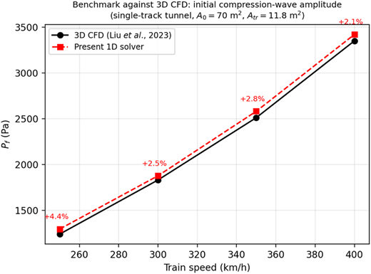
The grid-convergent output of the solver is benchmarked against an independent 3D-CFD dataset that is not used elsewhere in its construction. An independent 3D-CFD study (Liu, Liu, Yao, Chen, & Yang, 2023) reports, for a high-speed train in a single-track tunnel of A₀ = 70 m² (train area 11.8 m²), the initial compression-wave amplitude P_f as a function of speed from 250 to 400 km/h. Running the present solver at that configuration reproduces Pf to within 4.4% across the whole speed range, the deviation falling from +4.4% at 250 km/h to +2.1% at 400 km/h (Table 2, Figure 4) and captures the near-quadratic dependence on speed. This is an independent, high-speed benchmark on a configuration (single track, 70 m²) distinct from both the verification of Section 3.1 and the application of Section 4. It establishes the accuracy of the initial compression-wave amplitude only. The peak-to-peak load used in Section 4 is built on the same wave physics but additionally involves portal reflections, wave superposition, the tail expansion wave and friction over a full transit, none of which this comparison tests; that distinction is developed in Section 5, and no claim of equivalent accuracy for the complete pressure history is made here.

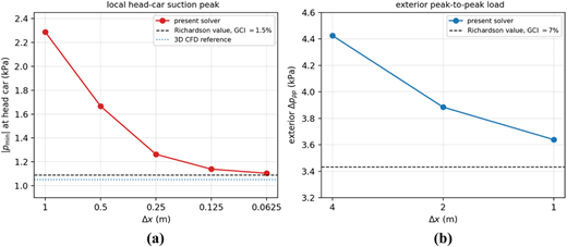
A formal grid-convergence study was performed following Roache's grid-convergence index (GCI, factor of safety 1.25) on systematically refined grids with refinement ratio 2. Two quantities are examined: the exterior peak-to-peak load used in Section 4, and the localised minimum (suction) pressure beneath the train nose in a benchmark configuration, which is the quantity most often used for point-value comparison with 3D CFD. The benchmark configuration is that of the moving-mesh 3D-CFD study of Luo et al. (2017): an eight-car train of length 200.68 m, maximum cross-sectional area 11.43 m² and streamlined head of 3.73 m, running at 200 km/h through a 500 m double-track tunnel of 80 m² free cross-section, with the pressure sampled 15 m behind the nose. It is distinct from the configurations of Sections 3.1 and 3.3 and from the application of Section 4. The raw values on every grid level are listed in Table 3, and the refinement behaviour is plotted in Figure 5, so that convergence can be inspected directly rather than through a single index.

The central result is that the nose suction peak is grid-convergent, but only on grids substantially finer than those normally used for wave-system work. The prescribed nose ramp of this benchmark is 3.73 m long, so grids of 1 and 0.5 m place only a few cells across the ramp; the triplet (1, 0.5, 0.25 m) accordingly lies in the pre-asymptotic range, returning an observed order of 0.63 and an apparent GCI above 70%. Refining further, the successive changes fall from 37% to 32%, 11% and, finally, 3.1%, the observed order rises to 1.70 and then 1.83 – approaching the formal second order of the scheme – and the fine-grid GCI falls to 6.0% and then 1.5%. The Richardson-extrapolated value, 1,084–1,091 Pa on the two finest triplets, lies within 3.5% of the 3D-CFD reference value of 1,054 Pa for the same configuration (Luo et al., 2017). A large GCI on a coarse triplet therefore indicates under-resolution, not the absence of a finite limiting solution; an earlier assessment based only on the (1, 0.5, 0.25 m) triplet reached the opposite conclusion and is corrected here.

Two checks separate numerical under-resolution from artefacts of the discretisation itself. Doubling or halving each Jameson dissipation coefficient (k₂ between 0.4 and 1.6, k₄ between 0.004 and 0.016) changes the peak by less than 0.7%, so the grid trend is not a dissipation artefact. Replacing the cosine nose ramp with a linear ramp of the same length changes the peak by 2.0% at Δx = 0.25 m and 1.2% at Δx = 0.125 m, a difference that itself diminishes under refinement, so the trend is not an artefact of the ramp representation either. A third check addresses the suggestion that only a spatially averaged peak might converge: averaging the pressure over windows of 1 m and 5 m centred on the probe changes the peak by less than 0.5% and leaves the GCI unchanged because in an area-averaged formulation the suction peak is a smooth feature distributed over the nose ramp rather than a singular spike. Spatial filtering is therefore unnecessary once the ramp itself is resolved. For the application train of Section 4, whose nose ramp is 12 m, the equivalent requirement is Δx of order 0.2–0.4 m; no point-value suction peak is reported for that configuration, and none of the results of Section 4 depends on one.

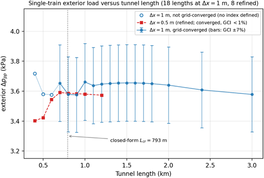
The convergence study was repeated at the edges of the design sweep, because the shortest tunnel and the largest blockage ratio need not share the resolution requirement of the baseline. At A₀ = 70 m², the behaviour matches the baseline (GCI 8.0% at Δx = 1 m). The shortest tunnel does not: for L = 0.5 km the triplet (4, 2, 1 m) returns a negative observed order (p = −1.52), so no meaningful index can be formed from it, and grids of Δx ≤ 1 m are required before convergence is attained, at which point the observed order is 2.88, and the load settles at 3.42 kPa with a GCI below 1%. All four grid levels for this case are listed in Table 3. The short-tunnel entries of the design sweep are therefore computed and reported at Δx = 0.5 m in Section 4.3, and the coarser resolution acceptable at 2 km is not sufficient there.

The resolution needed to converge the nose peak, Δx of order 130th to 160th of the nose ramp length, is roughly an order of magnitude finer in cell size than that needed for the wave-system load, and, because both the cell count and the number of explicit time steps scale with it, the corresponding cost is roughly two orders of magnitude higher. The practical consequence is a division of labour rather than a limitation of principle: the solver is used at Δx ≈ 1 m for the parametric work of Section 4, where only wave-system quantities are required and refined locally when a point-value peak is of interest. The remaining physical restriction is separate from resolution – the formulation carries no local (form) loss coefficients at the nose, tail or portals, so the converged peak is the inviscid area-averaged value, which the comparison above indicates is about 3.5% conservative relative to 3D CFD for this configuration.

For completeness, a moving-mesh 3D-CFD dataset (Luo et al., 2017) (head-car minimum pressure versus tunnel length at 200 km/h) is retained as a trend-level cross-check. That comparison is computed at Δx = 0.25 m, at which this quantity is not yet grid-converged (Table 3), so it is trend-level only: the 1D values exceed the 3D ones by between 4% and 20%, with the largest excess at the shortest tunnel. The 1D and 3D curves are nevertheless of the same order, and both exhibit an unfavourable-length plateau, though they place the shallow maximum at different lengths; the unfavourable length is determined directly in Section 4.3 instead of being inferred from this quantity.

The planned line is designed for 350 km/h with about 10% of its 1,541 km alignment in tunnels (National Assembly of Vietnam, 2024). The rolling stock is an eight-car CR400AF-type trainset (length 201.4 m, cross-section 11.2 m², perimeter 13.3 m, 12 m nose), and the baseline is a double-track tunnel of 100 m² free cross-section, with 70–100 m² examined for the cost–load trade-off (Table 4). All results are for a single train and, following Section 3, are reported as the grid-convergent exterior peak-to-peak pressure at Δx = 1 m (fine-grid GCI ≈ 7% at the baseline). Two-train crossings, which on a double-track line approximately double the loads and govern the comfort-based sizing, are outside this single-train scope and are treated in companion work; the conclusions below are conditioned accordingly.

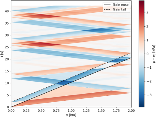
For the baseline (2 km, 100 m², 350 km/h), Figure 6 shows the pressure histories at a fixed mid-tunnel point and on the train body, and Figure 7 the corresponding x–t wave diagram. The grid-convergent exterior peak-to-peak load is 3.64 kPa at Δx = 1 m (Richardson value 3.43 kPa, fine-grid GCI 7.0%), formed as defined in Section 2.3 from the raw moving-probe history. The relevant design criteria are collected in Table 5. The exterior peak-to-peak value maps to the medical (health) limit; the interior comfort limits are reached by the cabin pressure, which depends on rolling-stock sealing and is assessed in Section 4.5 through a first-order sealing model.

Figure 8 shows the exterior peak-to-peak load against tunnel length. Following Section 3.4, the short-tunnel range is computed at Δx = 0.5 m, where the load is grid-converged, while the full range to 3 km is shown at Δx = 1 m with error bars given by the fine-grid GCI. For a single train, the load is remarkably insensitive to length: across 0.4–3 km it stays within about 5% of 3.6 kPa and across the refined range 0.7–1.2 km it varies by only 0.5%. Every value lies far below the 10 kPa medical limit.

Because the solver is available, the unfavourable (most severe) tunnel length is determined numerically rather than taken from the closed-form relation alone. On the refined grid the load rises monotonically from 3.40 kPa at 0.4 km to a shallow maximum of 3.59 kPa near 0.7–0.8 km and then decays slowly, which brackets the closed-form estimate L_cr ≈ (L_tr/4)(c₀/V)(1 + c₀/V) = 793 m adopted in the EN 14067–5 framework (CEN, 2021). The closed-form relation is thus confirmed by the solver for this configuration. Two qualifications matter for practice. The maximum is a broad plateau rather than a sharp peak – the metric changes by less than 1% between 0.7 and 1.2 km – so the unfavourable length is not a critical design threshold for the single-train exterior load. And on the coarser Δx = 1 m grid, the sweep shows an apparent maximum at 0.4 km, which the refined calculation removes; the variation across lengths is of the same order as the discretisation error at that resolution, which is why the refined grid is necessary for this particular question.

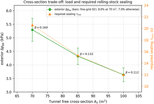
Figure 9 and Table 6 show what happens when the free cross-section is reduced from 100 m² (β = 0.112) to 70 m² (β = 0.160) for the 2 km tunnel. The exterior peak-to-peak load rises from 3.64 to 5.30 kPa, an increase of about 46%, reflecting the strong dependence of wave amplitude on blockage ratio; all three sections remain below the medical limit for a single train. Comparing the two sweeps, cross-section changes the load by an order of magnitude more than length does over the ranges examined, so among the parameters varied in this single-train study the cross-section is the stronger driver. This ranking is conditional on the parameters held fixed – speed, nose geometry, friction closure, portal configuration and single-train operation – and is not a general statement about all design variables.

The load alone does not express the trade-off a designer faces because the exterior load is not itself a comfort criterion: what the passenger experiences is the cabin pressure, which depends on how well the rolling stock is sealed. Table 6 therefore couples the three quantities that actually trade against one another. Reducing the section from 100 to 70 m² saves about 30% of the excavated volume, but raises the exterior load by 46% and, more demandingly, raises the sealing time constant required to meet the UIC comfort criteria from 12.0 to 20.6 s, an increase of 72%. The intermediate section of 85 m² saves 15% of excavation for a 28% increase in the sealing requirement. Since the sealing performance of the rolling stock is fixed by procurement rather than by the tunnel designer, this coupling is the practically binding constraint: a narrower tunnel is affordable in civil terms only if the fleet specification can carry the corresponding sealing requirement. The excavation figures are an order-of-magnitude proxy (free cross-section multiplied by length, excluding overbreak, lining and portal works) and are intended for relative comparison, not for costing.

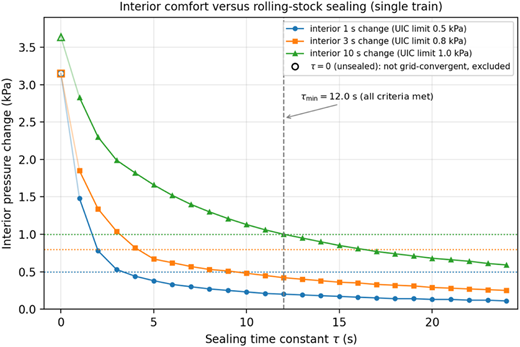
Passenger comfort is governed by the cabin pressure rather than the exterior pressure. The cabin pressure is obtained from the baseline exterior signature through the first-order sealing model of Section 2.4, and Table 7 and Figure 10 give the largest interior pressure change in the 1 s, 3 s and 10 s windows as a function of the sealing time constant τ.

Grid convergence was examined for each window separately rather than for the 3 s window alone, because the three windows weight the exterior transient differently. The unsealed case requires particular care: at τ = 0 the cabin pressure is identical to the exterior pressure and receives no filtering at all, and it is correspondingly not grid-convergent – between Δx = 2 and 1 m the three window metrics still change by 12.2%, 15.7% and 6.8%. Every sealed case is convergent: for τ ≥ 3 s, all three windows agree to within 0.4% across Δx = 4, 2 and 1 m. The first-order filter is a low-pass that attenuates precisely the sharp, grid-sensitive part of the exterior signal, so the interior metrics are a reliable model output in the sealed regime even where the raw exterior short-window metric is not. The results below are reported only for the sealed regime.

For the single-train baseline, the UIC criteria are met only by well-sealed stock. An unsealed vehicle fails by a wide margin; τ = 6 s satisfies the 1 s and 3 s limits but not the 10 s limit; and the 10 s criterion remains binding throughout the sealed range. The minimum sealing time constant satisfying all three criteria was located by bisection rather than read from a coarse sweep, giving τ_min = 12.05, 12.00 and 11.97 s at Δx = 2, 1 and 0.5 m respectively – that is, τ_min ≈ 12.0 s with a grid-related spread below ±0.05 s. The value of exactly 1.00 kPa in the 10 s column of Table 7 is not a coincidence: at the threshold, the binding criterion is met with equality by construction. Modern high-speed rolling stock lies within this range, so the baseline section is compatible with commercially available sealing performance. These conclusions are conditional on the first-order sealing model, which is the standard engineering representation but is not itself validated against measured interior pressure here (Section 5).

The evidence in this paper is of two different strengths, and it is worth stating which is which. The compression-wave amplitude – the quantity generated as the train enters the tunnel – is the best supported: it is verified against the analytical solution to within 1% over the blockage range used here, and it agrees with published 3D CFD to within 4.4% between 250 and 400 km/h. The piston-wind field is validated against a full-scale measurement on an operating high-speed line, the nose-passage transient being reproduced to within 2% in amplitude and 0.06 s in timing. The piston-wind field is supported by comparison with full-scale measurement (Section 3.2): the computed wind ahead of the train is low by 11%, the nose-passage minimum is reproduced to within 2% and the wave kinematics to within 0.06 s. The exterior peak-to-peak load used in Section 4 is a weaker claim. It is grid-convergent, and it is built from the same wave physics, but it also depends on portal reflections, wave superposition, the tail expansion wave, friction and the sampling trajectory, none of which is separately validated here. Agreement for the initial wave does not by itself establish equivalent accuracy for the complete pressure history, and the peak-to-peak results are therefore presented as a screening quantity with a stated numerical uncertainty rather than as a validated design value. Comparison against a measured pressure history – as distinct from the measured velocity history used in Section 3.2 – remains the most valuable next validation step.

Because the definition of the peak-to-peak metric affects both the convergence study and the comparison with design criteria, it is stated explicitly. It is formed from the pressure history at a probe moving with the train at mid-train length, over the interval from tunnel entry until the train has fully left the tunnel, as the difference between the maximum and minimum of that single history. It is not maximised over several probe positions. Wave amplitudes quoted elsewhere are plateau values, extracted as the median over 0.2–0.7 s after front arrival, which excludes the dispersive overshoot at the wave front (Figure 6). The peak-to-peak metric does not inherit that treatment: it is taken from the raw history, so the dispersive ringing that accompanies each front is included in it. This is deliberate, since a design load should not be reduced by a smoothing operation applied after the fact, and it makes the reported values conservative; but it is also the principal reason why this metric converges more slowly than the plateau amplitude, a fine-grid GCI of 7.0% against below 0.5% (Sections 3.1 and 3.4).

The remaining limitations bound the model rather than invalidate the results above. The formulation carries no local (form) loss coefficients at the train nose and tail or at the portals. Section 3.4 shows that this does not prevent the nose suction peak from converging – the converged value is about 3.5% conservative relative to 3D CFD for the benchmark configuration – but it does mean the model returns the inviscid area-averaged peak, and three-dimensional portal-relief effects are absent. The latter matters most for the shortest tunnels, where the portal region occupies the largest fraction of the domain; the 0.4–0.5 km results carry the largest physical uncertainty in Figure 8 for that reason, over and above the numerical uncertainty shown by the error bars. Adding calibrated loss-coefficient junctions, following established 1D practice (Vardy, n.d.; Woods & Pope, 1981), is the natural next development.

The study is single-train throughout. Two-train crossings approximately double the loads on a double-track line and govern both the structural sizing and the comfort assessment in practice; they require the two-blockage extension and are treated separately. No conclusion here should be transferred to a crossing scenario. Interior comfort is included through the first-order sealing model, whose output is grid-convergent in the sealed regime (Section 4.5), but which is not compared with measured cabin pressure in this work; the sealing conclusions are conditional on that model. The friction closures use constant Darcy coefficients; the piston-wind check of Section 3.2 is the only quantity materially sensitive to them and is not used in the application. The pressure-gradient output also provides the source term for micro-pressure-wave estimates (Baron et al., 2001; Howe, 1998), which are not pursued here.

On computational cost, the screening metric of Section 4 is converged at Δx ≈ 1 m, at which a single tunnel transit runs in tens of seconds on one processor core; resolving the local nose peak takes roughly two orders of magnitude longer but remains a matter of minutes. An equivalent moving-mesh 3D-CFD case of the kind used for the comparisons here requires multi-million-cell meshes and wall-clock times of the order of days on a cluster (Liu et al., 2023; Luo et al., 2017). A controlled like-for-like benchmark was not run, so the comparison is quoted as the difference in practical turnaround reported for such cases rather than as a measured speed-up factor; the point is simply that the 1D solver makes multi-case parameter studies routine, which is its intended role.

An open-source, MIT-licensed quasi-one-dimensional solver for piston-effect pressure waves in high-speed railway tunnels has been developed and released together with a reproducible verification-and-validation suite. The compression-wave amplitude is verified against the analytical solution to within 1% over a range of blockage ratios and agrees with published 3D CFD to within 4.4% between 250 and 400 km/h.

The grid study yields the principal methodological result. The localised head-car suction peak, commonly assumed to lie beyond the reach of area-averaged 1D models, is in fact grid-convergent: refined to a cell size of order 130th to 160th of the nose ramp length, it attains an observed order approaching the formal second order of the scheme, a fine-grid GCI of 1.5%, and a Richardson value within 3.5% of 3D CFD. What had appeared to be non-convergence was under-resolution of the nose ramp. Sensitivity tests on the artificial dissipation, the ramp representation and spatial filtering exclude the alternative explanations. The resolution requirement, however, is roughly an order of magnitude finer in cell size – and some two orders of magnitude more expensive – than that needed for wave-system loads, which sets a practical division of labour: coarse grids for parametric screening, local refinement for point-value peaks.

Applied to the planned 350 km/h North–South railway in Vietnam for a single train, the exterior peak-to-peak load varies by only a few per cent across tunnel lengths from 0.4 to 3 km, with a broad and shallow unfavourable-length plateau near 0.7–0.8 km that confirms the closed-form EN 14067–5 estimate of 793 m. Cross-section is the stronger of the two drivers examined: reducing the free section from 100 to 70 m² raises the load by about 46%. Coupled to a first-order sealing model, the design trade-off is sharper than the load figures alone suggest – that 30% saving in excavated volume raises the sealing time constant required for UIC comfort compliance from 12.0 to 20.6 s, so the narrower tunnel is viable only if the fleet specification can carry it.

It is equally important to state what this work does not provide. It is not a validated tool for train-crossing scenarios, which govern the design of double-track lines and lie outside the present single-train scope. Its evidence base covers the initial compression-wave amplitude and the piston-wind field; the complete-transit peak-to-peak load is grid-convergent and physically consistent but has not been compared with a measured full pressure history and is offered as a screening quantity. Local suction peaks are convergent but are returned without local loss mechanisms, so they should be read as inviscid area-averaged values, and short-tunnel results carry additional physical uncertainty from unmodelled portal relief. The sealing conclusions are conditional on a first-order cabin model that is not validated against measured interior pressure. Readers requiring point-value structural loads, crossing scenarios or portal-region detail should couple this solver with 3D CFD or measurement rather than substitute it for them.

The solver, its verification-and-validation suite and every application case are released openly so that the loss-coefficient, crossing and sealing extensions identified above can be developed and benchmarked by others on a common, reproducible baseline. That baseline, rather than any single numerical result, is the contribution this paper is intended to make.

During the preparation of this work, the author used an AI to assist with language editing and figure preparation. The author reviewed and edited all output and takes full responsibility for the content of the publication.

The author gratefully acknowledges the developers of the open-source scientific Python ecosystem – NumPy, SciPy and Matplotlib – on which the released solver and its verification-and-validation suite are built.

The supplementary material for this article can be found online